Optimization of Non Destructive testing when assessing stationary stochastic processes

HAL Id: hal-01008622

https://hal.archives-ouvertes.fr/hal-01008622

Submitted on 5 Jan 2019

HAL is a multi-disciplinary open access

archive for the deposit and dissemination of

sci-entific research documents, whether they are

pub-lished or not. The documents may come from

teaching and research institutions in France or

abroad, or from public or private research centers.

L’archive ouverte pluridisciplinaire HAL, est

destinée au dépôt et à la diffusion de documents

scientifiques de niveau recherche, publiés ou non,

émanant des établissements d’enseignement et de

recherche français ou étrangers, des laboratoires

publics ou privés.

stationary stochastic processes

Trung-Viet Tran, Franck Schoefs, Emilio Bastidas-Arteaga, Géraldine Villain,

Areaga Bastidas

To cite this version:

Trung-Viet Tran, Franck Schoefs, Emilio Bastidas-Arteaga, Géraldine Villain, Areaga Bastidas.

Op-timization of Non Destructive testing when assessing stationary stochastic processes. Fiabilité des

matériaux et structures (JFMS’12), 2012, Chambéry, France. �hal-01008622�

Revue. Volume X – n° x/année, pages 1 à X

"Optimisation de contrôles CND lors de l’auscultation d’un champ stationnaire de propriétés aléatoires (Optimization of Non Destructive testing when assessing stationary stochastic processes)", Fiabilité des matériaux et structures (JFMS’12), Session 1: Modèles de dégradation, inspection, maintenance, 10 p., Chambéry 4-6 juin 2012, Proc. on CD (2012).

Optimisation de contrôles CND lors de

l’auscultation d’un champ stationnaire de

propriétés aléatoires

Optimization of Non Destructive testing

when assessing stationary stochastic

processes

Trung Viet Tran*, Franck Schoefs*, Emilio Bastida-Arteaga*,

Geraldine Villain

**

_{Xavier Derobert}

**

* LUNAM Université, Université de Nantes,

Institute for Research in Civil and Mechanical Engineering, CNRS UMR 6183/FR 3473, Nantes, France

Franck.Schoefs@univ-nantes.fr

** LUNAM Université, IFSTTAR, MACS, Nantes, France

ABSTRACT. The localization of weak properties or bad behavior of a structure is still a

challenge for Non Destructive Testing (NDT) tools development and Structural Health Monitoring (SHM) design. In case of random loading or material properties, this challenge is arduous because of the limited number of measures and the quasi-infinite potential positions of local failures. Deterministic algorithms and specific multi-sensors systems are developed to this aim. In that case, generally, the precision of the positioning of a defect goes with a lack of sizing. However, the stochastic field is rarely a pure white noise and has a stochastic structure and probabilistic properties. These properties should be used to provide rational aid tools for optimizing the number of sensor. The paper shows that the stationary property is sufficient to find the minimum quantity of sensors and their position. A measure of the quality of information is suggested and the illustration is performed on a one-dimensional Gaussian stochastic field.

1. Introduction

Structural health monitoring is well recognized since at least two decades to provide valuable information for:

- structural model updating; - material property updating;

- monitoring of degradation and maintenance optimization; - loading analysis and modelling;

- survey of critical quantities in the structure.

The scope of the paper takes place in this last family where a decision should be made from a set of measure of a material property (yield strength, elasticity modulus) or a mechanical quantity of interest (strain, stress) Z. In a lot of cases, the material properties are random and two questions must be addressed: where is the defect and what is the probability of this event. Then the decision lies on a risk analysis that combines this measure of probability with the subsequent potential consequences, directly or after a structural reliability computation. In this last case, the question of random variable updating has been widely addressed during the two last decades. Random variable updating is very useful when data from inspections or monitoring are collected for condition assessment and reliability updating (Straub and Faber, 2003; Schoefs et al, 2012). Basically, the Bayes theorem and its derivative tools (Bayesian Networks) offer the theoretical context to deal with this issue. The so-called Risk Based Inspection (RBI) generalizes these approaches in the case of non-perfect inspections by linking inspection and decisions Faber, 2002; Sorensen and Faber, 2002; Schoefs et al, 2011). RBI methods are powerful once (i) there is no stochastic field involved into the problem, or (ii) the location of the most critical defect, from a reliability point of view, is known. In circumstance (i), if the field of Z is a white noise, the number of measures should tend to infinity. In practical cases, the building of large structures (soil, concrete, composite) generates a stochastic field for Z and its probabilistic properties should be used. Recently authors have combined structural reliability computation and stochastic field description in view to carry out a complete reliability analysis Stewart and Al-Harthy, 2008; Tran et al, 2012). The input of these works is the complete description of the stochastic field.

No work combines actually the two challenges: description of the stochastic field with a limited number of data and the structural reliability. This paper aims to suggest a methodology for the first one. The stochastic field could take several forms more or less complicated. The most simple is the stationary stochastic field that can be used, for instance, to model chloride distribution or other concrete properties (Bazant and Novak, 2000a; 2000b; Bazant and Xi, 1991). Other models suggest piecewise stochastic fields (Schoefs et al, 2009a, 2009b). The complexity comes from hazards B during building itself and from the spatial distribution of external factors E -e.g. environmental conditions. Within this context, the main objective of this work is to find the optimal geo-position of sensors and their number to satisfy a given level of quality when a stationary field can describe the stochastic field and the noise of measurement can be neglected.

2. Probabilistic modeling of measurements in case of spatial variability 2.1. Scope of the paper: stakes and limits

The interest of SHM checked out by this paper is to get a direct (so called non-model based) decision from the measurement and to detect:

- even the worst case;

- or the distribution of the worst cases (probabilistic distribution tails). The quantity of interest Z(B(x, θ),E(x, θ)) is supposed to be dependent of the

hazard during building represented by the stochastic field B(x, θ) and external

factors E(x, θ) where x denotes the vector of position and q is the hazard: θ ∈ Ω

where

_Ω

is the probabilistic space supposed to generates all the event that influence even B(x, θ) or E(x, θ). For simplicity, it is written Z(x, θ) in the following. We note

ˆz(x,θ

_i

)

one realization after measurement. When the quantity of interest is spatially dependent and no additional information is available for characterizing the potential position of a weak region, the question is to select at which position the measurement should be done. When Non Destructing Testing tools are carried out during service life, adjustments of the protocol (position, setting of the device…) can be suggested progressively with time.

When we have to design an embedded network of sensors (scope of the present paper) the device should be the solution of an optimization problem where the quality of the data encourages increasing the number of sensors when the cost reduction tends to limit their quantity.

In this paper we consider that a solution can be obtained only if the structure of spatial variability is known. He we assume that the stochastic field is stationary (probability density function is the same whatever the location) with a known fluctuation parameter (correlation parameter) but an unknown probability density function. So we assume:

- the measured quantity can be modeled with a stationary stochastic field: as a consequence, µz and σz are constant whatever x and parameter x will be

used when necessary only.

- the stochastic field is assumed to be Gaussian i.e. the considered property is normally distributed whatever the position;

- the measure is perfect in the sense that statistics moments computed from the set of ˆz(θi)

,

i

∈

[

1

,...,

N

]

tend to the probabilistic moments of Z(θ)

when Nž ∞;

- a quality of the measurement can be expressed even on the form [1], [2] or [3]:

Confidence interval, when the distribution of values around the mean value is

[

]

(

Z Z Z Z

)

z I a th z S

_p

_P

_P

_z

P

P

εµ

µ

εµ

µ

−

+

∈

=

≥

,

,ˆ

ˆ

;

ˆ , [1] where

P

_S,zˆ is the probability computed from the sensor measurements,P_th the theoretical probability (implicitly non null), and pa denotes the minimum acceptable probability to get a measurement

zˆ

inside a given range governed by the exact value of the expectation µz and an error around this mean value computed by the percentage ε. Note that

zˆ

can be replaced by its statistics like the mean value or standard deviation when statistical error (i.e. samples of small size) is investigated (Schoefs et al, 2011a; Tran et al, 2011).

Distribution of extreme values, left side, when extreme low values (strength) is

analysed,

(

Z Z

)

z I a th z S

z

P

P

p

P

P

εµ

µ

−

≤

=

≤

,

,ˆ

ˆ

ˆ , [2]

Distribution of extreme values, right side, when extreme high values (stress) is

studied,

(

Z Z

)

z I a th z S

_p

_P

_P

_z

P

P

εµ

µ

+

≤

=

≥

,

,ˆ

ˆ

ˆ , [3] Equations [1], [2] and [3] are compatible with a lot of numerical post-treatment algorithms for detection assessment.

Note that, at this stage no mechanical model is s-used (model free or non model based approach) and we consider a one-dimension (1D) field for illustration. Of course the methodology can be expanded to any stationary stochastic fields: 2Dor 3D.

Let us assume that we get a set of independent realizations –i.e. structural components-ˆz(θi)of Z(θ). From a huge number of data (N≈1000), PS, ˆzcan be

estimated directly from the frequency of measurements only if it is not too small. When only a limited number of data is available (N<100), we have to assess the empirical distribution from a numerical sampling knowing the empirical distribution: it can be reached by using Monte Carlo Markov Chain. The number of components being limited the stake will be to get independent realization Ns on a

given component and to consider a set of components Nt.

Here we compute P_{S, ˆz}by considering the probability density function with parameters µ_Zˆ and σ_Zˆcomputed from the empirical distribution of measurements:

( )

_∑

(

)

∑

= =

−

=

=

N i Z i Z N i i Z

_N

z

_N

z

1 ˆ ˆ 1 ˆ

ˆ

(

,

)

(

)

1

)

,

(

ˆ

1

)

(

x

x

θ

σ

x

x

θ

µ

x

µ

;

[4]

This variable is denoted

Zˆ

. In the following, the challenge will be to consider a model of spatial variability and to assess a set of independent realizations of Z(θ)

2.2. Spatial variability

Risk Based Inspection analysis or reliability methods applied to real structures generally assume:

- either there is no spatial variability involved in the problem: random variables allow us to describe the hazard involved;

- or the location of the most critical defect from reliability point of view is known and the distribution of defects in its neighboring doesn’t affect the reliability.

It is well known that the reality is more complex and that we should account for stochastic fields too. Then the stochastic field could take several forms more or less complicated:

- (i) the most simple is the stationary stochastic field that is able to model the chloride distribution or other properties in the concrete for instance (Bazant and Novak, 2000a; 2000b; Bazant and Xi, 1991);

- (ii) more sophisticated is the piecewise stationary process that can integrate the variability of the con-creating by steps or the corrosion of structures in contiguous but different environments;

- (iii) finally, fully non stationary fields are certainly the most acceptable for a fine representation of properties.

However, except for natural soils, materials used for construction (airplanes, bridges …) are produced following a quality process and control. We can consider that some variation are fair, for instance the spatial change of the mean value. This paper focuses on the first model (i) only.

In this paper, we used a Karhunen–Loève expansion to represent the spatial variability with this assumption of stationary (Schoefs et al, 2011c):

)

(

).

(

.

.

)

,

(

1

x

x

_i n i i i Z Z

f

Z

_∑

=

+

=

µ

σ

λ

ξ

θ

θ

[5]

where, n is the number of terms in the expansion, ξi is set of centered reduced

Gaussian random variable (standard normal variables), λIand

f

i are respectively the

eigenvalues and eigenfunctions of the covariance function: ρ(Δx) . The major interest of this representation is that λi and fi have analytical expressions for specific

forms of the correlation function.

For instance, let us consider a one-dimensional (in space) stochastic field (x=x)withan exponential form of correlation function as follows:

0

;

exp

)

(

⎟

>

⎠

⎞

⎜

⎝

⎛ Δ

−

=

Δ

with

b

b

x

x

ρ

[6]

Then, it is shown that eigenvalues and eigenfunctions λi and fi have analytical

expressions (see Tran et al. 2012b):

2.3. Assessment of the autocorrelation function from measurements

We assume that the stationary stochastic field can be characterized by an autocorrelation function (ACF). Table1 presents the most usual ACF considered for spatial variability of structures with their parameter, called scale of fluctuation δ. A

complete overview of the auto-correlation functions and their application is available in Kenshel (2009). Let us focus on the assessment of this function from experimental data (sensors or NDT tests).

Two major procedures have been reported in the literature for the estimation of δ

for a spatially variable property from a digitized record of data. In the first procedure, reported by Li (2004), the Maximum Likelihood Estimate method (MLE) is used in which different values for the model parameter of the proposed ACF model is assumed and the value that maximizes the corresponding MLE is taken as the model parameter. In the second procedure, proposed by Vanmarcke (1983), a proposed ACF model (Tran et al. 2012b) can be adjusted to provide the best fit to the actual sample correlation coefficients ρ(Δx) thereby providing estimates of the corresponding model parameter (i.e. b in [6]).

In this paper, we select an exponential ACF [6]. and we use the likelihood estimate for the estimation of b.

⎟

⎟

⎟

⎟

⎠

⎞

⎜

⎜

⎜

⎜

⎝

⎛

−

⎟⎟

⎠

⎞

⎜⎜

⎝

⎛

=

⎟

⎟

⎠

⎞

⎜

⎜

⎝

⎛

⎟

⎟

⎠

⎞

⎜

⎜

⎝

⎛

−

=

∑

∏

= =

2

exp

2

1

2

exp

2

1

1 2 1 2 k i i k k i i

L

ν

π

ν

π

[7] where νi is the ith component of the vector of independent standard values obtained

from equation:

⎟⎟

⎠

⎞

⎜⎜

⎝

⎛ −

=

− Z Z

z

C

σ

µ

ν

1 [8]

where z is the vector of realizations of the random variable Z and C a lower triangular matrix such that CCT= ρ and ρ the autocorrelation matrix. Beside, maximize L is equivalent to minimize L1:

∑

=

=

k i i

L

1 2 1

ν

[9]

3. Optimization of geo-position of sensors 3.1. Optimization problem description

In this paper, we consider a one-dimensional mechanical problem with a set of sensors to be equally distributed with distance δI on Nt structures of length L(beams

of a bridge, cables, wing of an airplane, …). The optimization problem is written as a minimization problem of the number of sensors for a structure with a finite length

L. In fact the question is to find the minimum number of sensors Ns in each

component knowing the number of components Ntunder one of the constraints [1]

to [3].

N

S

=

min

(

N

s

(

1

)

or

(

2

)

or

(

3

)

)

[10]

In a complete risk analysis it can be written:

* argmin, ( ( )) C E N N N Nt Ns t S = = _[11]

where E(C) denotes the expectation of the cost (Schoefs, 2009).

3.2. Study case

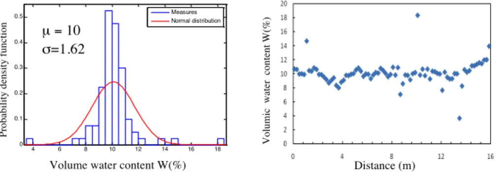
In this part, we consider the optimization of position and number of inspection for assessing the volume water content W (%) in a reinforced concrete beam by capacitive method (CAPA). Its main characteristics are 16 meters length, 1 meter height and 0.4 meter width. A grid has been drawn on each lateral surface and 2 lines of measurement have been selected: distance from the top line and the first line of measurements is 7 cm and distance between two lines is 20 cm. Distance between each measurement on one line is 20 cm.

3.3 Data analysis

With CAPA method, we get a value of the frequency F. The difference ΔF between the frequency in air and on concrete can be related to the permittivity of concrete from a calibration function given by IFSTTAR (Schoefs et al. 2012): it depends mainly on the size of the electrode. He we used a “great electrode” without Eccostock and calibration function is given in [12].

9711

.

26

7937

.

22

+

−

=

Δ

F

Eps

[12]

where ΔF = Fc - Fair, with Fc and Fair values of frequencies in RC beam and in the

air on site. And, volume water content W can be deduce from permittivity by a second calibration function [13] (see Schoefs et al. 2012).

61 . 4 64 . 0 + = W Eps [13]

Figure 1 presents the distribution of W after post-treatments for records along a line (left) and the spatial distribution of theses data (right). These data correspond to the mean value of 30 repetitive tests at each position. The scatter is low in comparison to the inherent scatter of the measurement: Schoefs et al. (2012) have recorded a standard deviation up to 2.5 for repetitivity tests.

Figure 1: Spatial variability of measure W and its distribution at line B

3.4 Results of optimization

For the structure considered in this paper, very close values of L1 [9] are

obtained for the two lines: 1.63 and 1.61m respectively for the B and the A line. For this paper, we focus to optimization positioning and number of captor on the RC beam when considering a stochastic stationary Gaussian field of volume water content W with its parameter µW = 10 and σW = 1.62.

- length of beam: L = 16 m.

-

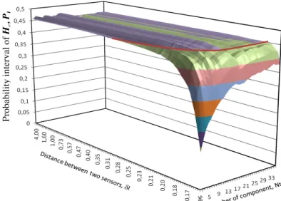
parameter of autocorrelation function: b = 1.62 m. And the distance between two captors varied from 0.1 to 5m.

First, let us consider the case with repetitive tests (i.e. without noise of measurement), and constrain [1] were ε=1(%). For a normally distributed random variable Pth=0.463 andPS, ˆz ≥ 0.42. Figure 2 presents the variations of PS,hcwith the

number of components (beams) Nt and distance between inspections δI; δI varying

from 0.16 (Ns=100) to 4 (Ns =4). This figure shows that the probability increases

Pr oba bi li ty de ns it y fu n ct io n

Volume water content W(%) Distance (m)

Vo lu m ic wa te r co n ten t W (% ) 4 6 8 10 12 14 16 18 0 0.1 0.2 0.3 0.4 0.5 Measures Normal distribution µ = 10 σ=1.62

according to the number of component Nt and decreases according to distance of δI.

Based on this result, for a given accepted valueP_{S, ˆz}, we obtain a curve that links the acceptable couples (δI; Nt) (see red line in Figure 1 for

P

_S,_zˆ=0.42). Note that if Nt is

too small there could be no solution (for instance for

P

_S,zˆ=0.42).

Figure 2

:

Influence of Nt and δI in probability interval

P

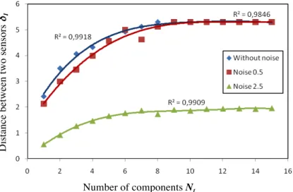
S,zˆof W

Figure 3 presents this curve for PI=42% and its fitting with a power function (red line). Based on this result, given Nt, we obtain the distance between two captors δI following [14]:

δ

_I

=

0

.

921

( )

N

_t 0.4327 [14] and the position and minimum number of sensors are deduced. For example, for Nt=10,δI=2.2m and Ns=16/2.2 = 7.27 measure on each component, and the total number of sensor is: N=10*7=70 captors.

Pr o b ab il it y i n te rv al o f Hc , P I

Figure 3: The curve of Nt and δI satisfying PI =42%

Let us considered now the absence of repetitive tests: noise of measurement exists (see Rouhan et al. 2003 for definition). Based on preliminary results (Schoefs et al. 2012) we focus study on two value of the standard deviation of a centered normally distributed withe noise: 0.5 and 2.5. The later figure presents this result for the case ε=3σW = 4.68 and for PI=90% where we show the predominant role of

the noise especially when it is higher than the standard deviation of the signal itself..

Figure 4: The curve of Nt and δI considering the noise measurement satisfying PI

=90% Di st an ce be tw ee n tw o sen so rs δI Number of components Nt Di st an ce be tw ee n tw o se n so rs δI Number of components Nt

4. Conclusions.

This papers aim to focus on the first step of a work dealing with uncertainty in measure assessment and intrinsic spatial variability. Only the case of stationary Gaussian fields of properties is investigated herein. It is shown how to model a stationary stochastic field and to follow up this property to get a good representation of a random variable from a limited number of NDT measurements. We developed an illustration based on capacitive measurements with and without error of measurements. This result can be exploited in further reliability updating once the first measurements are available.

5. Bibliographie

Bazant Z. P., Novák D., “Probabilistic Nonlocal Theory for Quasibrittle Fracture Initiation and Size Effect. I: Theory”, Journal of Engineering Mechanics. 2000a ,Vol. 126, No. 2, 166-174.”

Bazant Z. P., Novák D., Probabilistic Nonlocal Theory for Quasibrittle Fracture Initiation and Size Effect. II: Application”, Journal of Engineering Mechanics, 2000b. Vol. 126, No. 2, 175-185.

Bazant Z. P., Xi Y., “Statistical Size Effect in Quasi-brittle Structures: II. Nonlocal Theory”,

ASCE J. of Engrg. Mech. 1991, Vol. 117, No. 11, 2623-2640.

Faber M.H., “Risk Based Inspection: The Framework”. Structural Engineering International (SEI), 12(3), August 2002, pp. 186-194.

Gomes, H. M., and Awruch, A. M., “Reliability of reinforced concrete structures using stochastic finite elements”, Engineering Computations, 2002, 19(7-8), 764- 786.

Kenshel O.M., “Influence of spatial variability on whole life management of reinforced concrete”. PhD Thesis, University of Dublin, Trinity College, August 2009.

Li, Y., “Effect of spatial variability on maintenance and repair decisions for concrete structures”, PhD thesis, Delft University, Delft, Netherlands. 2004

Mark G.S., and Ali Al-Harthy., “Pitting corrosion and structural reliability of corroding RC structures: Experimental data and probabilistic analysis”. Rreliability Engineering and

System Safety, 2008, 93, 373-382.

Rouhan, A., Schoefs, F. Probabilistic modelling of inspections results for offshore structures. Structural Safety, Vol. 25, 2003, pp. 379-399.

Schoefs F., Tran T.V., Bastidas-Arteaga E., “Optimization of inspection and monitoring of structures in case of spatial fields of deterioration/properties”. Applications of Statistics

and Probability in Civil Engineering, Taylor & Francis Group, London, ISBN

978-0-415-66986-3. 2011c

Schoefs F., Boéro J., Clément A., Capra B., “The αδ method for modeling expert Judgment and combination of NDT tools in RBI context : application to Marine Structures”.

and performance (NSIE), Special Issue “Monitoring, Modeling and Assessment of Structural Deterioration in Marine Environments”, accepted January 2010, Vol. 8, N° 6,

April 2012, pp. 531-543, doi: 10.1080/15732479.2010.505374.

Yuan X.-X, Pandey M.D., “Analysis of approximations for multinormale integration in system reliability computation”, Structural Safety, 2006, 28, 361-377.

Sørensen J.D. and Faber M.H., “Codified Risk-Based Inspection Planning”. Structural

Engineering International (SEI), 12(3), August 2002, pp. 195-199.

Schoefs F., Yáñez-Godoy H., Lanata F., “Polynomial Chaos Representation for Identification of Mechanical Characteristics of Instrumented Structures: Application to a Pile Supported Wharf”. Computer Aided Civil And Infrastructure Engineering, spec. Issue “Structural

Health Monitoring”,Volume 26, Issue 3, pages 173–189, April 2011b.

Schoefs F., Clément A., Nouy A., “Assessment of spatially dependent ROC curves for inspection of random fields of defects”.Structural Safety, Vol. 31, Issue 5, September 2009, pp. 409-419

Schoefs F., “Risk analysis of structures in presence of stochastic fields of deterioration: coupling of inspection and structural reliability”. Australian Journal of Structural

Engineering, Special Issue “Disaster & Hazard Mitigation”, 2009, Vol. 9, N°1, pp.

67-78.

Schoefs F., Tran T.V., Villain G., Derobert X., Bastidas-Arteaga E., “Optimization of NDT measurement for stochastic fields: application to capacitive measurement on e concrete

beam”, ICDS 2012 – Durable Structures, from Construction to rehabilitation, Lisbon, Portugal – 31st _may-1st _{june 2012, 2012.}

Schoefs F., Tran T.V., E. Bastidas-Arteaga., “Optimization of inspection and monitoring of structures in case of spatial fields of deterioration/properties”. 10th International Conference on Applications of Statistics and Probability in Civil Engineering – ICASP 2011, Switzerland, August 1-4, 2011a

Stewart M.G., and Al-Harthy A., “Pitting corrosion and structural reliability of corroding RC structures: Experimental data and probabilistic analysis”. Reliability Engineering and

System Safety, 2008, 93, 373-382.

Straub, D., Faber, M.H., “Modelling dependency in inspection performance”, Proc.

Application of Statistics and Probability in Civil Engineering, ICASP 2003 – San

Franncisco, Der Kiureghian, Madanat and Pestana eds., Mill-press, Rotterdam, ISBN 90 5966 004 8. pp. 1123-1130.

Tran T.V., Schoefs F., Bastidas-Arteaga E., Villain G., Derobert X., “Optimization of NDT measurements for structural reliability assessment in case of spatial variability”, International Workshop « Non Destructive Testing and Evaluation: Physics, Sensors, Materials and Information », November 21-22 2011, Ecole Centrale de Nantes, France. Tran T.V., Bastidas-Arteaga E., Schoefs F., Bonnet S., O’Connor A.J., and Lanata F.

“Structural reliability analysis of deteriorating RC bridges considering spatial variability”. 6th International Conference on Bridge Maintenance, Safety and Managements – IABMAS 2012, Italy, July 8-12, 2012a.

Tran T.V., Schoefs F., Bastidas-Arteaga E., Villain G., Derobert X., “Optimization Of Geo-positioning Of Sensors In Case Of Spatial Fields Of Deterioration/Properties”, EACS

2012 – 5th European Conference on Structural Control , paper #212, 11 pages, Genoa, Italy – 18-20 June 2012, 2012b.

Vanmarcke, E., “Random fields: analysis and synthesis”, MIT Press, Cambridge, Mass; London. 1983.

Vanmarcke, E., and Grigoriu, M., “Stochastic Finite Element Analysis of Simple Beams”.

Journal of Engineering Mechanics, 1983, 109(5), 1203-1214.

View publication stats View publication stats