Monitoring of the upstream part of a supply chain dedicated to the customized mass production with a revisited version of MRP

(1)

Laboratoire d'Analyse et Modélisation de Systèmes pour

l'Aide à la Décision

CNRS UMR 7243

CAHIER DU LAMSADE

316

Janvier 2012

Monitoring of the upstream part of a supply chain

dedicated to the customized mass production with a

revisited version of MRP

V. Giard, M. Sali

(2)

Abstract: This article focuses on the monitoring of a supply chain dedicated to the mass production of strongly

diversi-fied products. Specifically, we are interested in the part of this chain that contributes to the production of a set of alter-native modules assembled on a work station of one or several assembly lines, whose production levels are stable. The MRP approach is adopted for the monitoring of this chain. The distance between the production units leads to a mix between production to stock and production to order. In this article, we establish the relations that allow us to define, in a steady state, the quantities to produce that address the requirements of the Master Production Schedule and that are partially or completely random to limit the stockout risk to a very low predetermined level. We will distinguish two cases by accounting for, or not accounting for, problems that are related to quality.

Keywords: MRP, Make To Stock, Safety Stock, Supply Chain, Order Penetration Point.

1 Introduction

In the real world, for Supply Chains (SCs) dedicated to the mass production of strongly diversified products that are characterized by a certain geographical dispersion of the production units of the SC, production is determined by several distant final assembly lines with a stable daily production (at least in the course of a few weeks). Diversity is provided mainly by the assembly of alterna-tive modules (e.g., engines, gear boxes) on several workstations of the assembly line. Each station is dedi-cated to a different set of alternative modules, of which one must be mounted on the end product processed by this station. The optional modules (e.g., the sliding roof) can be treated as a specific case of the alternative mod-ules. Several examples of this type of SC can be found in the automotive industry.

When the total daily production volume is certain, the daily requirement for all of the systematically assem-bled parts and the components that they use is also cer-tain. The control of these flows is relatively easy in the absence of risk related to the quality of the components, the transportation time or the production time.

For the alternative modules and the components that they use, the flow control is more complex. We are interested here in piloting the production units of these modules and the components that they use under the assumption that customer orders to suppliers are ad-dressed simultaneously with the same periodicity. The operating process used is Manufacturing Resource Planning (MRP), for which planned orders of the com-ponents are determined by a backward simulation that combines a mechanism of explosion of the Bill Of Ma-terial (BOM) with a mechanism of lead time offset. In MRP, the Master Production Schedule (MPS) plans the production of all of the supply chain units that manufac-ture the modules and components included in the end products.

After a brief review of the literature (§1), a revisited version of the MRP will be proposed (§2) and then numerically illustrated (§3). In conclusion (§4), we will describe the conditions that must be guaranteed for applying this approach efficiently.

2. Literature review

MRP was initially proposed to be implemented in a deterministic environment; no securing method was initially imagined. The confrontation of this idealized perception of planning with the real world highlighted the necessity of dealing with the uncertainty of certain information that is used within the framework of the MRP model. At the end of the 1970s, attempts to adapt the MRP method to an uncertain environment were suggested.

The first source of uncertainty that was studied was related to the demand. To address this concern, (Büchel, 1982) models uncertainty with random variables and calculates, on each level of the BOM, the variance of the demand for the components, leading to the possibil-ity of calculating safety stocks. The problem of the components that are common to several end-products is managed by considering that their demands are random variables whose variances are the sums of the variances of the requests. The implicit assumption of demand independence does not hold if it concerns a component that is common to a subset of alternative modules be-longing to a given set of alternative modules mounted at the same workstation of the final assembly line. Indeed, it is shown below (see §2) that the probability distribu-tion of the demand for a component common to several components of a subset of alternative modules is a weighted sum of binomial distributions; this relationship invalidates the property of the variance additivity. Based on a case study, (De Bodt & al., 1982) evaluate the effectiveness of the use of safety stocks in MRP with uncertain demands. Their level and localization result from a simple comparison between several sce-narios: no determination method is presented in this article.

(Winjgaard & al., 1985) describe the principles and advantages of the use of the safety stock, of the safety lead time and of the increase in the quantities of the MPS. A dimensioning method for the safety stocks is provided for serial, convergent and divergent configura-tions of the supply chain. The authors only consider the case of components that are related to the end-product by a BOM coefficient equal to 1 without accounting for the commonality.

(3)

(Lagodimos & al., 1993) examine the problem of the localization of the safety stocks in the MRP of standard-ized products. Their objective is to maximize the service level by distributing among the various levels of the BOM a given value of safety stock by using an analyti-cal approach. It is considered here that the service level is not a decision variable and that the holding costs are identical for each level of the BOM. This assumption is strong given that the value of a component usually de-creases with its BOM level. The proposition goes in the direction of a placement of the safety stock on the level of the end-products for the serial structure of a supply chain. Nevertheless, the authors relativize their results by pointing out the limits imposed by the assumptions of their modeling.

Under the assumption that demands are usually distrib-uted in the steady state, (Inderfurth & al., 1998) are interested in the double problem of the dimensioning and the localization of the safety stocks of components. The goal of this study is to reach a given service level (size and duration of stockout) at each level of the sup-ply chain while minimizing the overall carrying costs. They propose a model of optimization that respects a service level that ensures the decoupling of the supply chain units. The requirements of a component come from the final MPS demand and could be related to one or more different end products. In this last case, correla-tions between demands are introduced to model the requirements of the studied component. This approach is not valid if that component is mounted in different alternative modules that belong to the same set of alter-native modules.

On the basis of the holding cost and service rate, (Zhao & al., 2001) compare the performance of three dimen-sioning methods for calculating the safety stock. Ac-counting for the results realized by (Carlson & al., 1986), they decided to place the safety stock at the level of the end product. For each of the three methods, a different demand cover time is used for the calculation of the safety stock. No justification is given to defend the choices.

In a more recent article, (Persona & al., 2007) propose an analytical method for dimensioning safety stocks of components or modules in the case of a production or assembly to order. In their modeling, they consider a steady state in which the procurement lead times are certain and the demands for alternative components are correlated within the same family of alternative mod-ules. The concept of correlation used in this article re-fers to the statistical link that exists between the de-mands relating to alternative modules of the same set

j

E

. This relation is the result of a constraint based on the multinomial distribution and is not the result of a correlation between random variables. Correlations exist between alternative components that belong to different sets, but they are only important in the case of a compo-nent that is used to link two alternative modules that belong to two different sets of alternatives (junction components).

(Winjgaard & al., 1985), (Guerrero & al., 1986), (Buzacott & al., 1994), (Molinder, 1997) and (Chang, 1985) explored other strategies for protection against uncertainty in the MRP environment such as raising the requirements of the MPS or lengthening the lead times artificially. (Buzacott & al., 1994) are interested in the possibility of using safety lead times as a means of pro-tection against uncertainty. They consider that a trade-off must be made between safety stocks and safety lead times according to the reliability of the forecasts, the production capacities, the holding costs and the stockout costs. They consider in their modeling only one MRP echelon operating in an uncertain environment. The conclusion from this study is that safety stocks reduce the total costs in the event of strong uncertainties on the demand. The safety lead time has the ability to antici-pate a known demand to come and necessarily leads to an increase in a stock at a level that depends on the period length.

In a similar study, (Molinder, 1997) proposes rules for decision making to help choose between safety stocks and safety lead times. The parameters of the decision refer to the degrees of uncertainty of demand and lead times and the ratio between the stockout costs and hold-ing costs. Its conclusions are somewhat different from those made by (Buzacott & al., 1994) in that he recom-mends the use of safety lead times in the event of strong uncertainties of both demand and lead times. One can note that the cost that is associated with a safety lead time is induced by an increase in the stocks and that consequently, the opposition between the safety stock and the safety lead time is not very clear.

Exploring other ways for dealing with uncertainty in MRP, (Zhao & al., 1993) propose to freeze the master production schedule in a high proportion according to parameters related to the planning horizon and the re-planning periodicity. This solution, conceivable in a make to stock context of standardized products, is unus-able in a make to order production of diversified prod-ucts.

Many literature review articles relating to MRP have been published in the 2000s. To clearly highlight fields not yet explored by the specialized literature and to clarify the positioning of our work compared to what has already been accomplished, it is interesting to check the analysis framework used by these literature reviews. (Guide & al., 2000) are interested in the techniques used to counter uncertainty in MRP. The analysis framework comprises the following seven axes: the modeling pro-cess, the dimensioning method for the safety stocks, their localization, the definition of the safety lead time, the type of uncertainty accounted for in the model, the nature of the planning horizon (rolling or fixed), and finally, the key performance indicator that is retained. The examination of the literature in this article leads to the conclusion that several gaps still exist even if certain suggested solutions remain applicable, according to the

(4)

LAMSADE Cahier 316

Vincent Giard & Mustapha Sali

authors, under a set of assumptions that are sometimes debatable. These authors also regret the lack of method-ology and the absence of precise rules that allow for the establishment of a compromise between the various suggested alternatives for protection.

Another categorization of the literature is proposed by (Koh & al., 2002), in which the analysis is performed on three axes. In the first axis, the authors distinguish be-tween the inside risks that are related to the processes and the outside risks. The second axis is related to the point of occurrence of the risk, which can be upstream or downstream in relation to the productive process. Last, the third axis relates to the type of solution that is recommended to mitigate the risk through safety stocks or techniques, such as an increase in the quantities of the MPS. The interesting conclusion from this article is that very few studies address the interactions between several sources of risk.

More recently, (Dolgui & al., 2007) propose an analysis of articles that relate to the management of the risk in MRP. The articles selected are classified into three categories based on the type of the risk taken: the de-mand, the lead time and a combination of both. The authors briefly present some of the techniques that are commonly used to control the consequences of uncer-tainty, namely the frozen horizon, safety stock and safe-ty lead times. Aside from the limitations highlighted by this study and those identified by (Guide & al., 2000) and (Koh & al., 2002), they emphasized that there are very few articles that address the MRP replannification in multi-echelon configurations.

The risk that is taken in the productive part of SC, treat-ing the procurement of optional or alternative compo-nents (and the compocompo-nents that they use) for assembly lines dedicated to the mass production of customized products, presents several specific characteristics that have not yet been considered in the literature and that we will attempt to develop.

3. The MRP model revisited

3.1 Treatment uncertainty in the traditional

approach of the MRP

The frozen horizon H_F is the initial part of the plan-ning horizon H_Pon which the demands of the first periods of the MPS (from t to t+HF − ) are intangible. 1 This concept is related to that of the Order Penetration Point (OPP), which delimits what can be made to order from what is to make to stock (Vollmann & al., 1997). This separation, obvious in the SC convergent network, is less clear in a divergent network that characterizes an SC that has several distant assembly lines. In this case, a part mounted on those lines could be partly made-to-order (MTO) and partly made-to-stock (MTS), depend-ing on the distance between the assembly lines and the plant that produces that component.

The application in the cascade of the BOM explosion results in finding a_ik units of reference i, of the BOM level n, included in the reference k pertaining to the subset E of the MPS (level 1 of the BOM). In addi-_ik tion, the application in the cascade of the mechanism of the lead times offsets leads to a lag λ_ik between the period t of launching into production, the reference i and the period t+λ_ik for the use of the reference k in the MPS. This scenario makes it possible to bind the gross requirement GR_it to a reference i of level n of the no-menclature at period t, with the demands MPS_kt′of reference k (level 1 of the nomenclature) at periods

t′ >t_{and not with the planned orders of the references}

of level n′ <n_{of the nomenclature, which use that}

reference i directly (which is typical in an MRP). To establish this relation, it is advisable to notice that, in a deterministic universe (non-revisable MPS, absence of quality problems, deterministic lead times), the on-hand balance OHB at the end of the period t for any refer-_it

ence i must be null because, in this deterministic con-text, a stock generates a cost without any useful coun-terpart. Consequently, the planned order PO_it for the reference i at the beginning of the period t is necessarily equal to the quantity _,

i i t L

q

₊ , which is delivered at the beginning of period t+L_i, taking into account the lead time L_i of this reference i. In its turn, _,

i i t L

q

₊ is neces-sarily equal to the net requirement _,

i i t L

NR

₊ for this period, which is equal to the gross requirement _,

i i t L

GR

₊

for this same period. These various values are linked to the requirements of the MPS by the relation (1).

, _i , _i , _i it i t L i t L i t L

PO

=

q

₊

=

NR

₊

=

GR

₊ , _ik ikaik MPSk t+λ =

∑

E ⋅ (1)

The reference i is entirely made-to-order if

Max (

)

F

k

λ

ik

≤

H

, which corresponds to the “regular”

case of MRP use. The reference i is entirely made-to-stock if

Min (

)

F

k

λ

ik

>

H

because the MPS

require-ments used in this relation are unknown. Last, a mix of MTO and MTS occurs when the reference i is linked with at least a reference k such as λ <_ik H_F and with at least a reference k' such as λ_ik_′≥H_F. The latter case, which is not treated, to our knowledge, in the literature on the OPP or on MRP, is important to consider because it is quite common in the modern world SC, such as in the automotive industry.

A company can use an MTO policy to control the pro-duction of a set of references that are manufactured on various sites belonging to its SC only if it has an OPP that is defined on a frozen horizon, such as

,

Max ( )

F i k ik

H ≥ λ . By increasing the lags λ_ik, the replacement of nearby suppliers by remote suppliers can lead insidiously to the non-observance of that condition

(5)

and, thus, can trigger a loss of flow control in the SC, unless this reference is partially (or completely) made-to-stock with appropriate rules to avoid stockouts. In this type of SC, the diversity of the end-products is too important to allow the MPS to be defined at the level of the end-product. The MPS must be defined at the level of the alternative modules. The planning BOM

c



of a set of K alternate modules describes the average structure for the use of these alternative modules by a set of end-products that are assembled on the same line. It is necessary to define as many planning BOMs as there are assembly lines using these alternative compo-nents because of the difference in the structure of the demand that must be met. The elements of this vector c correspond to the average proportions c_k of the con-sumption of the modules K; obviously,

∑

k K_k=₌₁ c_k =1. This vector c_{can be regarded as the vector of} probabil-ities for the use of the alternative modules in the steady state to characterize the demands X of the alternative modules beyond the frozen horizon. The random de-mand of the alternative modules X follows the Multi-nomial distribution

M

( , )

N c



, in which N is the daily production of the line. The daily demand X_k of the module k follows the Binomial distribution B ( ,N c_k), in which the complementary event to “use module k” is to “use another alternative module”.

3.2 MRP in an MTO/MTS environment

without a quality problem

The flow synchronization in the type of SC studied here can depend on the MPR if its rules can be adapted to calculate the planned orders of a component i, which depends on MPS requirements going beyond the frozen horizon (∃λ_ik≥H_F,k∈E_ik). When there are lags of these alternative modules k such as λ_ik≥H_F, the part of the production of component i that is induced by these requisitions must be made-to-stock. It is advisable, then, to replace the notation _,

ik k t

MPS

₊_λ , which is suita-ble for a known demand of the alternative module k for the period t+λ_ik, by the random variable _,₊_λ

ik k t

X

,

which is replaced by X_k if the characteristics of the steady state remain stable over the planning horizon. In that case, the gross requirement _,

i i t L

GR

₊ is defined by relation (2), as follows: , i ik _ik H_F , ik i t L ik k t GR + =∑E _λ _< a ⋅MPS +λ , _ik ikλ_ik≥H_Faik Xk t+λ +∑_E ⋅ (2)

In the logic of the MRP, the planned delivery _,₊

i i t L

q

(equal to the planned order LP ) corresponds to the net _it

requirement _,

i i t L

NR

₊ of this reference i for this period + _i

t L , which is equal to the gross requirement

GR

i t L,+ _i

for this period, minus the projected available inventory

, i 1 i t L

AI

_{+ −} at the end of the previous period t+L_i−1. This projected inventory _, ₁

i i t L

AI

_{+ −} depends on the on-hand balance OHB_{i t}_,₋₁ at the end of the period t− and 1 on the gross requirements and planned deliveries of the periods t to t+ − : Li 1 1 , _i 1 , 1 i , , t t L i t L i t t t i t i t AI + − =OHB − +∑′=′= + − q ′−GR ′_ (3) Then, in the determination of the planned delivery

,+ _i i t L

q

, it is necessary to integrate uncertainty relating to the gross requirement _,

i i t L

GR

₊ and to the projected inventory _, ₁

i i t L

AI

_{+ −} . The quantity to be delivered at the beginning of the period is then the sum of a known

quantity _,

ik ikλ_ik<H_F aik⋅MPSk t+λ

∑E and a quantity

defined as the difference between an order-up-to level

,+ i i t L

R

and a deterministic projected available invento-ry _, ₁

i i t L

AI

′

_{+ −} , which is derived from relation (3) in which only the deterministic part of GR_{i t}_,′ is used. Then, _,₊

i i t L

R

corresponds to the fractile, which is asso-ciated to the stockout risk α of a probability distribution of a demand _,₊ i i t L

Y

(P(

_, _,

)

i i i t L i t L

Y

₊

>

R

₊

=

α

. The demand _,₊ i i t L

Y

corresponds to the sum of the random requirements of the periods t+ to 1 t+L_i, with the gross requirement GR_it of the first period being neces-sarily known. Given that the MPS requirements of the module k for the period t+λ_ik−h are unknown, if

ik h HF λ − ≥ , then _,₊ i i t L

Y

is defined by relation (4), as follows: 1 , i 0i ik ik F , ik h L i t L h H h ik k t h Y ₊ =∑ = −₌ ∑_E _λ _≥ ₊ a ⋅X ₊_λ ₋ (4) Therefore, the planned order PO_it of reference i, which is equal to the planned delivery _,₊

i i t L

q

at period t+L_i, is the sum of the following:

- The deterministic requirement for period t+L_i, i.e.,

, _ik

ikλ_ik<H_F aik⋅MPSk t+λ

∑E ,

- The difference between _,

i i t L

R

₊ and _, ₁ i i t L

AI

′

_{+ −} . Then, the planned order PO is defined by relation (5), _it

as follows: , _i _ik _H , _ik , _i ik F it i t L ik k t i t L PO q a MPS R λ < λ + + + = =∑_E ⋅ + 1 , 0 [ h Li it h i t h it OHB = −₌ q ₊ GR − +∑ − ₁i 1 _, ] ik ik F ik h L H h ik k t h h λ a MPS λ = − < + + − = −∑ ∑E ⋅ (5)

(6)

LAMSADE Cahier 316

Vincent Giard & Mustapha Sali

The production of the entire made-to-stock is a special case of relation (5), in which

, 1

ik ik F i

k λ H L

∀ ∈E ≥ + − , to make random all of the gross requirements for the period t+ to 1 t+L_i. In that case, no deterministic requirement of MPS stands, and the relation (6) is to be used.

1 , i , i 0i , h L it i t L it i t L it h i t h PO =q ₊ =GR +__R ₊ −OHB − ∑ ₌= −q ₊ __ with λ ≥ik HF+ − ∀ ∈ELi 1, k ik (6)

In the steady state, R_it′=R_i,∀t′. R_i can be drawn from relation (5), for period t, with

q

it′

=

LP

i t L,′− _i

,

∀

t

′

and

can be replaced by that expression in that relation for period t+ . After simplification, one obtains relations 1 (7) and (8), which are more convenient to use in the steady state than the relations (5) and (6). Because the deterministic part of the MPS requirements vary with the used horizon, a superscript is necessary to notate precisely at what initial period the analysis of the future requirements is performed. , i it i t L it

PO

=

q

₊

=

GR

1 0 , 1 i ik ik F ik h L t H h ik h λ a MPSk t λ h = − < + = − + − +∑ ∑_E ⋅ 1 1 0 , 1 i ik ik F ik h L t H h ik h λ a MPSk t λ h = − − < + = − + − −∑ ∑_E ⋅ (7) , _i it i t L it

PO

=

q

₊

=

GR

(Steady state and ∀ ∈k E_ik, λ_ik≥H_F +L_i−1) (8) A change of the steady state at period

Max (_k _ik)

t+ λ modifies the order-up-to level. This change is progressive and lasts for Max (_k λ −_ik) H_F

periods. During that transitory state, the difference be-tween the new value for the order-up-to level and the previous value is to add to the relations (7) and (8) for calculating the planned order.

3.3 MRP in an MTO/MTS environment

with a quality problem

Let us assume that no quality problem occurs for all of the components that include component i of level n, until the modules k of level 0, and that the quality is checked before the departure of the deliveries.

If the gross requirement _,

i i t L

GR

₊ to be met by the planned order PO_it is known (λ <_ik H_F,∀k), then it is possible to protect against a stock shortage by the possi-bility that each produced part has the probapossi-bility π_i of nonconformity, through a safety stock ̶ or Target Stock ̶ TS_i, defined as the fractile _,

i

i t L

Uα′₊ specified for the stockout risk α′ of the random variable _,₊

i i t L

Z

, which follows the Negative Binomial distribution

,

(

,

)

i i t L i

GR

₊

π

NB

. , _i ( _ik _H , _ik, ) ik F i t L ik k t i Z _λ a MPS _λ π < + ∼NB ∑E ⋅ + i i t L, i

TS

U

₊

→

=

with

P(

_, _,

)

i i i t L i t L

Z

₊

>

U

₊

=

α

′

(9) Obviously, it is the variation of this target-stock

,+ _i

−

,+ −_i 1 i t L i t L

U

that is added to the gross requirement

, _i i t L

GR

₊ to calculate the planned delivery _,₊

i i t L

q

, if 1 > i

L ; otherwise, AOH_{i t}_,₋₁ replaces _, ₁

i i t L

U

_{+ −} . Then, relation (10) is to be used, as follows:

, _i _ik _H , _ik ik F it i t L ik k t PO q _λ a MPS _λ < + + = =∑E ⋅ _, _, ₁ i i i t L i t L

U

₊

U

_{+ −}

+

−

(10) The name “target-stock” is used here in preference to that of safety stock, which is defined classically as the difference between an order-up-to level and an average demand (which is not the case here). In the absence of defective pieces in the production that are launched in the period t, the projected inventory _,

i i t L

AI

₊ at the end of period t+L_i (after control and before expedition) is equal to this target-stock _,

i i t L

U

₊ .

The use of these relations implies that a calculation of the target-stock is made at each decision-making point. If the probability of nonconformity is weak, then a value for the stock-target will be valid for a relatively broad range of values of Gross Requirements, which allows an easy construction of a decision table that avoids repeat-ing the calculation each time.

If the gross requirement _,

i i t L

GR

₊ is completely or par-tially random, then the first argument of the Negative binomial distribution becomes random. The risk of nonconformity must be taken into account in the defini-tion of the order-up-to level _,₊

i i t L

R

because only one safety stock can be used. This risk sharing, by the simul-taneous consideration of uncertainties on the demand and quality, leads to don’t separate the origin of the stockout. Then, the order-up-to level _,₊

i i t L

R

is defined by relation (11) and is calculated by using the Monte Carlo method, as follows:

, ,

P(

)

i i i t L i t L

W

₊

>

R

₊

=

α

where _, _, _, i i i i t L i t L i t L

W

₊

=

Y

₊

+

Z

₊ , 1 , i 0i ik ik F , ik h L i t L h H h ik k t h Y ₊ =∑ = −₌ ∑_E _λ _≥ ₊ a ⋅X ₊_λ ₋ and , i

(

, i i t L i t L

Z

₊

∼ NB

Y

₊ , 0i ik ik F ik , ) h L H h ik k t h i h λ a MPS λ π = < + + − = +∑ ∑E ⋅ (11)

The exact solutions of relations (10) and (11) oblige us to compute the probability distributions _,₊

i i t L

Z

or

, i i t L

W

₊ at every decision-making point. In the steady state, if π_i is weak, then it is simpler to regard Z_i or W_i

as random variables in which all of the requisitions of the MPS intervening in the calculation of the gross

(7)

requirement are random; then, relation (12) can be used, as follows:

(

_i _i

)

P W

>

R

=

α

with

W

_i

= +

Y

_i

Z

_i ( , ) i i i i Z ∼NB Y +Y′π 1 0i ik ik F h L i h H h ik k Y =∑ = −₌ ∑_E _λ _≥ ₊ a ⋅X 0i ik ik F h L i h H h ik k Y′=∑ =₌ ∑_E _λ _< ₊ a ⋅X (12) The generalization of the approach that accounts for the problems of quality in the production of the components

j of level n+ used by component i of level n is rather 1 simple at the level of the principles. This approach is, however, complicated to implement in practice because it does not lead to analytical relations as simple as those found above. It is necessary to continue the calculation of planned orders PO_it_′ for the periods t′ >t_{using the}

same approach as for the calculation of PO_it by distin-guishing the deterministic part from the random part. After that, it is necessary to calculate planned orders of the components j by adapting the approach that led to the relation (11).

4 Numerical example

Let us illustrate the use of these analytical relations through a fictitious example. We consider the produc-tive part of an automoproduc-tive supply chain that leads to two cars’ assembly factories (A and B) belonging to the same company. These two factories have a common engine supplier, which does not have other customers. The engine plant is supplied by a unique supplier of pistons and is its unique customer. The piston plant buys the piston crowns from a unique supplier, and it is also the supplier’s unique customer. It is assumed that these different plants use an MRP-I approach that shares a common periodicity (a time bucket of two days) for launching production and receiving deliveries.

Figure 1: BOM and lead time definition

Figure 1 describes the relevant extract of BOM for the studied subset and shows the lead times. At level 0, one finds that the vehicles manufactured by the two distant assembly plants are dedicated to different markets that do not have the same structure of demand. At level 1, one finds the planning BOM that is associated with each one of these lines; among the 5 alternative modules of the set E, only the engines E1 and E5 use the pistons that

are of interest here. The piston crowns are specific to

each type of piston. Lead times integrate times of pro-duction and transportation to the customer. The distanc-es between the assembly factoridistanc-es and the engindistanc-es plant are such that it is necessary to isolate a transportation lead time in the mechanism of MRP.

The MPS of factories A and B are defined at the level of the alternative modules (engines), in other words, at level 1 of the BOM. These data, as well as the initial on-hand balance and planned deliveries, are provided in table 1 (to see at the end of this article). In this example, it is easy to calculate the

λ

_ik values for the pistons, for example, for the piston crowns (see table 2). All of the calculations in the table below were performed by con-sidering that the frozen horizon length is 9 periods, with the result that one is under the normal conditions of use for MRP.

Alternative module k∈E_ik

1A

M M_{5 A} M_1B M_5B

ik

λ

, for i = piston crown 7 6 8 7

ik

λ

, for i = piston 5 4 6 5

Table 2: λ_ikvalues for the pistons and piston crowns

The analytical solutions suggested for determining the order-up-to level or the target-stock will be illustrated with a very low level of risk. This choice is justified by the seriousness of the economic consequences of stock-outs, which encourages taking expensive measures for meeting the demands to avoid the propagation of dis-turbances along the supply chain.

4.1 Production partly to stock in the

ab-sence of a quality problem

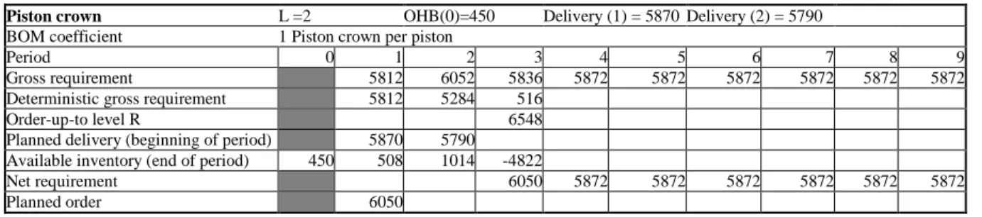
This scenario occurs when reference i is linked with at least a module k such as λ <_ik H_F and with at least a reference k' such as λ_ik_′≥H_F. With a frozen horizon of 7 periods, pistons are made-to-order, and piston crowns are made partly to order and partly to stock (see table 3). In table 1, information on the MPS corresponds to the expected values of the engine demands, beyond this 7th period. Table 3 links the gross requirements of the pis-ton crowns to the engine demands.

Table 3: Decomposition of the requirements of the pis-ton crown by engines MPS

(8)

LAMSADE Cahier 316

Vincent Giard & Mustapha Sali

The deterministic parts of the gross requirements of piston crowns (reference i) for periods 2 and 3 are 5284 and 516, respectively; GR_i₁( 5812)= is completely de-terministic (a firm order sent by the pistons factory). According to the relation (4), withL_i=2, the demand

3 i

Y

corresponds to the sum of the random requirements of the periods 2 to 3: 3 4 (960;0,2) 4 (1840;0,54) i Y = ×B + ×B 4 (960;0,2) 6 (960;0,1) + ×B + ×B . This distribution is a weighted sum of Binomial distributions and does not have an analytical solution. It is determined numerically without difficulty using the Monte Carlo simulation method. With a risk of 0.01%,

3

P(Y >6548) 0.0001= and the order-up-to level

R

_i₃ is 6548. 1,0% 98,0% 1,0% 5 796 6 376 5 600 5 800 6 000 6 200 6 400 6 600 6 800 0,000 0,001 0,002 0,003 0,004 0,005 0,006 0,007 Figure 2: Distribution of Y_i₃

The use of

R

_i₃ is illustrated in table 4 (see the end of this article), which shows, for a horizon passing from 9 to 7 periods, the calculation of the planned order of the piston crowns, the planned orders of the pistons and the engines that remain unchanged. The available inventory

2 1014

i

AI = at the end of period 2 (and thus at the be-ginning of period 3) is the difference between the sum of the initial on-hand inventory (450) and the expected deliveries (5870+5790) and the deterministic part of the gross requirements of periods 1 to 2 (5812 5284)+ . The planned order PO_i₁=q_i₃=6050 is the sum of the de-terministic part of the gross requirement of period 3 (516) and of R_i₃−AI_i₂=6548 1014 5534− = .

After having illustrated the use of relation (5), let us next illustrate relation (7), which is valid in the steady state. By performing the calculations for MRP one peri-od later (see table 5), the decision to be made at the beginning of period 2 depends now on the engine de-mands known for the periods 2 to 8. Let us suppose that, for this last period, the demands for the engines are

1 ,8A 991

MPS = , MPS_{5 ,8}_A =109 MPS_{1 ,8}_B =214 and

1 ,8

5_B 84

MPS = . In period 1, the deterministic part of the gross requirements of periods 2 and 3 was

5284 516 5800+ = ; in period 2, the deterministic part of the gross requirements of periods 3 and 4 is

4984 612+ =5596. In application of relation (7), the planned order PO_i₂ is equal to

6140 (5596 5800) 5936+ − = (the application of the relation (5) yields the same result =612 6548 1224+ − ).

4.2 Production in the presence of a quality

problem

To illustrate relation (9), it will be assumed that prob-lems of quality are encountered in the manufacturing of the pistons, with a risk of π =0.1% that a piston is regarded as defective after quality control. With a gross requirement of 6050 units for period 3 (see table 1), the target-stock is 17, as defined by the fractile of

,3 pistons

Z

∼

NB(6050;0,1%) for the risk α =0.01%. If the quality control, performed before sending the deliv-ery of 5780 pistons at the beginning of period 1, rejects 7 pistons, then the available inventory at the end of period 2 is decreased by 7, and the initial planned order (5812) is increased by 17 7 24+ = to reach 5836 units. It is interesting to note that the target-stock of 17 units is associated with a range of gross requirements from 5507 to 6269, which suggests the possibility of avoiding calculations by using decision tables that are easy to establish.

To illustrate relation (11), we suppose now that the production of engines and pistons are without defects and that the defect risk for a piston crown is still

0.1%

π = . The deterministic part of the gross require-ment remains 5812 5284 516 11612+ + = . The definition of

Y

_i₃ corresponds to the same sum of the random re-quirements of periods 2 to 3. Then, the distribution of

3

i

Z is ∼NB(11612+Y_i; 0,1%), and the distribution of

3

i

W =Y_i₃+Z_i₃ is obtained using a Monte Carlo simu-lation, from which one obtains P W( _i₃>6556) 0.01%= . This scenario yields the new order-up to level that pro-tects from the two sources of randomness.

5 Conclusions

Thus, it is possible to guarantee a good performance in piloting a supply chain dedicated to mass-customized production using a revisited approach of MRP that combines MTO and MTS, accounting for the risks of the demand fluctuation and the quality and allowing the use of different frozen horizons depending on the knowledge of the customers’ demands. Two observa-tions must be made with regard to the underlying as-sumptions that place conditions on the effectiveness of this approach.

The use of the planning BOM c of a set of K alternative modules assumes its stability. In the opposite case, it is necessary to anticipate the dated transformations of this structure that are induced by changes in the customers’ expectations or by marketing actions (limited series, promotions) of the company or its competitors. A regu-lar and rigorous analysis of these upcoming changes is essential; otherwise, the piloting of the supply chain will not remain under control. The costs of this information-al monitoring are low, taking into consideration those induced by a pilot and not ensuring decisional

(9)

coher-ence in the supply chain. The organization and the fol-low-up of this vigilance place a condition on the per-formance, even perennity, of the supply chain.

On the principles level, the mechanisms proposed are relatively easy to implement because it is a question of transmitting order-ups to levels and target-stocks. The implementation is more difficult when the concerned plants do not belong to the same company. A contractu-al agreement must then be proposed, accepted by contractu-all and implemented. An additional difficulty is related to the fact that a supplier of the supply chain can belong to several supply chains (Renault and PSA supply chains share many suppliers). Technically, the generalization of the suggested approach could be immediate if the same principles of piloting are retained by all, which makes it possible to pool the risk; however, this strategy then poses some problems in the contractual formula-tion because the safety stocks are calibrated for aggre-gated demands. A less efficient solution consists of regarding the customers of the same supplier as inde-pendent. In addition, it is advisable to not underestimate the problems of confidentiality that are involved by the sharing of information that is coming from several sup-ply chains.

(10)

LAMSADE Cahier 316

Vincent Giard & Mustapha Sali

MPS of engines E1 et E5 defined at the beginning of period 1

Period 1 2 3 4 5 6 7 8 9 A MPS(engine 1) 993 984 978 1001 979 976 1036 994 994 MPS(engine 5) 97 93 97 112 107 90 86 92 92 B MPS(engine 1) 171 198 183 184 193 188 205 192 192

MPS(engine 5) 117 94 82 105 113 114 100 96 96

TRANSPORT: 2 days from the engine assembly plant to the vehicle assembly plant A

4 days from the engine assembly plant to the vehicle assembly plant B

Period 1 2 3 4 5 6 7 8 9 Delivery at plant A Delivery (engine 1) 993 984 978 1001 979 976 1036 994 994 Delivery (engine 5) 97 93 97 112 107 90 86 92 92 Delivery at plant B Delivery (engine 1) 171 198 183 184 193 188 205 192 192

Delivery (engine 5) 117 94 82 105 113 114 100 96 96 Departures to plant A Expeditions (engine 1) 984 978 1001 979 976 1036 994 994 994 Expeditions (engine 5) 93 97 112 107 90 86 92 92 92 Departures to plant B Expeditions (engine 1) 183 184 193 188 205 192 192 192 192 Expeditions (engine 5) 82 105 113 114 100 96 96 96 96

Engine 1 L=2 OHB(0)=30 Delivery (1)=1190 Delivery (2 )=1200

Period 0 1 2 3 4 5 6 7 8 9 Gross requirement (E1 to be sent to A) 984 978 1001 979 976 1036 994 994 994 Gross requirement (E1 to be sent to B) 183 184 193 188 205 192 192 192 192 Total gross requirement 1167 1162 1194 1167 1181 1228 1186 1186 1186 Planned delivery (beginning of period) 1190 1200 Available inventory (end of period) 30 53 91 -1103 Net requirement 1103 1167 1181 1228 1186 1186 1186 Planned order 1103 1167 1181 1228 1186 1186 1186 1186 1186

Engine 5 L =1 OHB(0)=15 Delivery (1)=190

Period 0 1 2 3 4 5 6 7 8 9 Gross requirement (E5 to be sent to A) 93 97 112 107 90 86 92 92 92 Gross requirement (E5 to be sent to B) 82 105 113 114 100 96 96 96 96 Total gross requirement 175 202 225 221 190 182 188 188 188 Planned delivery (beginning of period) 190 Available inventory (end of period) 15 30 -172 Net requirement 172 225 221 190 182 188 188 188 Planned order 172 225 221 190 182 188 188 188 188

Pistons L =2 OHB(0)=20 Delivery (1) =5780 Delivery (2) =5900

BOM coefficient 4 pistons for engine 1 6 pistons for engine 5

Period 0 1 2 3 4 5 6 7 8 9 Gross requirement from E1 4412 4668 4724 4912 4744 4744 4744 4744 4744 Gross requirement from E5 1032 1350 1326 1140 1092 1128 1128 1128 1128 Total gross requirement 5444 6018 6050 6052 5836 5872 5872 5872 5872 Planned delivery (beginning of period) 5780 5900 Available inventory (end of period) 20 356 238 -5812 Net requirement 5812 6052 5836 5872 5872 5872 5872 Planned order 5812 6052 5836 5872 5872 5872 5872 5872 5872

Piston crown L =2 OHB(0)=480 Delivery (1) = 5870 Delivery (2) = 5790

BOM coefficient 1 Piston crown per piston

Period 0 1 2 3 4 5 6 7 8 9 Gross requirement 5812 6052 5836 5872 5872 5872 5872 5872 5872 Planned delivery (beginning of period) 5870 5790 Available inventory (end of period) 450 508 246 -5590 Net requirement 5590 5872 5872 5872 5872 5872 5872 Planned order 5590 5872 5872 5872 5872 5872 5872

XXX Pegging of pistons XXX Pegging of piston crown

Table 1: Illustration of the MRP calculus in a deterministic universe (H_F=9)

Period 0 1 2 3 4 5 6 7 8 9

Gross requirement 5812 6052 5836 5872 5872 5872 5872 5872 5872

Deterministic gross requirement 5812 5284 516

Order-up-to level R 6548

Planned delivery (beginning of period) 5870 5790

Available inventory (end of period) 450 508 1014 -4822

Net requirement 6050 5872 5872 5872 5872 5872 5872

Planned order 6050

(11)

Period 0 1 2 3 4 5 6 7 8 9

Gross requirement 6140 5752 5932 5872 5872 5872 5872 5872

Deterministic gross requirement 6140 4984 612

Order-up-to level R 6548

Planned delivery (beginning of period) 5790 6050

Available inventory (end of period) 508 158 1224 -4708

Net requirement 5936 5872 5872 5872 5872 5872

Planned order 5936 5872 5872 5872 5872 5872 5872

Table 5: Calculus of the planned order of piston crowns of period 2 (H_F=7- no quality problem)

References

Büchel, A. (1982) "An overview of possible procedures for stochastic MRP", Engineering Costs and

Production Economics, n° 6, pp. 43-51.

Buzacott, J.A. & Shanthikumar, J.G. (1994) "Safety stocks versus safety time in MRP controlled Production systemss", Management Science, Vol. 40, n° 12, pp. 1678-1688.

Carlson, R.C. & Yano, C.A. (1986) "Safety stocks in MRP-systems witht emergency setups for

components", Management Science, Vol. 32, n° 4, pp. 403-412.

Chang, A.C. (1985) "The interchangeability of safety stocks and safety lead time", Journal of Opertations

Management, Vol. 6, n° 1, pp. 35-42.

De Bodt, M.A., Van Wassenhove, L.N. & Gelders, L.F. (1982) "Lot sizing and safety stock decisions in an MRP system with demand uncertainty", Engineering

Costs and Production Economics, n° 6, pp. 67-75.

Dolgui, A. & Prodhon, C. (2007) "Supply planning under uncertainties in MRP environments: A state of the art", Annual Reviews in Control, n° 31, pp.269– 279.

Guerrero, H.H., Baker, K.R. & Southard, M.H. (1986) "The dynamics of hedging the master schedule",

International Journal of Production Research, Vol.

24, n° 6, pp. 1475-1483.

Guide, V.D.R.J. & Srivastava, R. (2000) "A review of techniques for buffering against uncertainty with MRP systems", Production Planning & Control, Vol. 11, n° 3, pp. 223 - 233.

Inderfurth, K. & Minner, S. (1998) "Safety stocks in multi-stage inventory systems under different service measures", European Journal of Operational

Research, n° 106, pp. 57-73.

Koh, S.C.L., Saad, S.M. & Jones, H.M. (2002) "Uncertainty under MRP-planned manufacture: review and categoriztion", International Journal of

Production Research, Vol. 40, n° 10, pp. 2399-2421.

Lagodimos, A.G. & Anderson, E.J. (1993) "Optimal positioning of safety stocks in MRP", International

Journal of Production Research, Vol. 31, n° 8, pp.

1797-1813.

Molinder, A. (1997) "Joint optimisation of lot-sizes, safety stocks and safety lead times in an MRP system", International Journal of Production

Research, Vol. 35, n° 4, pp. 983-994.

Persona, A., Battini, D., Manzini, R. & Pareschi, A. (2007) "Optimal safety stock levels of subassemblies and manufacturing components", International

Journal of Production Economics, n° 100, pp.

147-159.

Vollmann, T.E., Berry, W.L. & Whybark, D.C. (1997)

Manufacturing Planning and Control Systems, 4th

edition, New York, Irwin/McGraw-Hill. Winjgaard, J. & Wortmann, J.C. (1985) "MRP and

inventories", European Journal of Operational

Research, n° 20, pp. 281-293.

Zhao, X., Lai, F. & Lee, T.S. (2001) "Evaluation of safety stock methods in multilevel material

requirements planning (MRP) systems", Production

Planning & Control, Vol. 12, n° 8, pp. 794-803.

Zhao, X. & Lee, T.S. (1993) "Freezing the master production schedule for material requirements planning systems under demand uncertainty",

Journal of Operations Management, n° 11, pp.