Search for Compromise Solutions in
Multiobjective State Space Graphs
Lucie Galand and Patrice Perny
1Abstract. The aim of this paper is to introduce and solve new search
problems in multiobjective state space graphs. Although most of the studies concentrate on the determination of the entire set of Pareto optimal solution paths, the size of which can be, in worst case, ex-ponential in the number of nodes, we consider here more specialized problems where the search is focused on Pareto solutions achieving a well-balanced compromise between the conflicting objectives. After introducing a formal definition of the compromise search problem, we discuss computational issues and the complexity of the prob-lem. Then, we introduce two algorithms to find the best compro-mise solution-paths in a state space graph. Finally, we report various numerical tests showing that, as far as compromise search is con-cerned, both algorithms are very efficient (compared to MOA*) but they present contrasted advantages discussed in the conclusion.
1
INTRODUCTION
Traditionally, heuristic search problems in state space graphs are con-sidered in the framework of single objective optimization. The value of a path between two nodes is defined as the sum of the costs of its arcs and the problem amounts to finding one path with minimum cost among all paths from a source node to the goal. This problem is solved by classical constructive search algorithms likeA∗
[5] which provide, under certain assumptions, the optimal solution-path, using a heuristic function to concentrate the search on the most promising nodes and paths. Thus, during the search, preferences over sub-paths or nodes candidate to development are measured by a scalar evaluation function inducing a complete weak-order over competing feasible paths.
However preferences are not always representable by a single criterion function. Indeed, in many practical search problems con-sidered in Artificial Intelligence (e.g path planning, game search, preference-based configuration), comparison of solutions includes several aspects or points of view (agents, criteria, scenarios). In such problems, an action allowing a transition from a node to another is evaluated with respect to these different points of view, thus leading to multiple conflicting evaluations non-necessarily reducible to a sin-gle overall cost. For this reason, the vector-valued generalization of the initial problem have been investigated and several extensions of the so-called A∗
algorithm are now available. Let us mention, among others, MOA∗
the multiobjective extension of A∗
finding all Pareto optimal paths [13] and its recent refinement [9], U∗
a variation of A∗
used to find a maximal path with respect to a multiattribute utility function [2], ABC∗
to find paths which best satisfy a set prioritized goals [8] and finally preference-based generalizations of MOA∗
[6] and [10].
1LIP6 – University of Paris 6, France, email: [email protected]
As soon as several objectives must be optimized simultaneously, most of the studies concentrate on the determination of the entire set of Pareto optimal solutions (here solution-paths having cost vector that cannot be improved on a criterion without being degraded on another criterion). However, the size of the Pareto set in combinato-rial problems being often very large, its determination induces pro-hibitive response times and requires very important memory space.
Nevertheless, in many contexts, there is no need to determine the entire set of Pareto optimal elements, but only specific compromise solutions within this set. This is particularly the case in multiobjec-tive path-planning problems where the most preferred solution-paths are those achieving a good compromise between various conflict-ing objective (minimize time, energy consumption, risk,. . .). This is
also the case in vector-valued path problems issued from robust opti-mization. In such problems involving a single cost function, several plausible scenarios are considered, each having a different impact on the costs of transitions between nodes. The aim is to find a robust
path, that is a path which remains suitable in all scenarios (e.g the
minimax path [7, 11]). In such examples, the type of compromise solution sought in the Pareto set is precisely defined and this can be used to speed up the search.
When preference information is not sufficient to formulate a sta-ble overall preference model, iterative compromise search can still be used to explore the Pareto set. One starts with a “neutral” initial pref-erence model used to generate a well-balanced compromise solution within the Pareto set and the model progressively evolves with feed-backs during the exploration to better meet decision maker’s desider-ata. Such an interactive process is used in multiobjective program-ming on continuous domains to scan the Pareto set which is infinite, see e.g. [12]. The same approach is worth investigating in large size combinatorial problems when complete enumeration of the Pareto set is not feasible.
Motivated by such examples, we consider in this paper multiob-jective search problems in state space graphs with a specific focus on Pareto solution-paths achieving a good compromise between the conflicting objectives. After introducing the basic notations and defi-nitions used in the paper, we define formally the compromise search problem in Section 2 and discuss computational issues. In section 3 we recall the basic principles of MOA∗
and introduce two origi-nal algorithms to find the best compromise solution-paths in a state space graph. The first one, called BCA∗
(Best Compromise A∗
), is a variant of MOA∗
specially designed to focus directly on a target compromise solution. The second one called kA∗
achieves the same goal while working on a scalarized version of the problem. Section 4 is devoted to the presentation of numerical tests allowing the rela-tive performance of MOA∗
, BCA∗
and kA∗
to be compared, in the determination of the best compromise solution-paths.
2
COMPROMISE SEARCH
We introduce now more formally the framework of multiobjective optimization and compromise search in state space graphs.
2.1
Notations and Definitions
A∗
algorithm and its multiobjective extensions look for “optimal” paths (in some sense) in a state space graph G = (N, A) where N is a finite set of nodes (possible states), and A is a set of arcs
representing feasible transitions between nodes. Formally, we have
A = {(n, S(n)), n ∈ N } where S(n) ⊆ N is the set of all
suc-cessors of noden (nodes that can be reached from n by a feasible
elementary transition). Thens ∈ N denotes the source of the graph
(the initial state),Γ ⊆ N the subset of goal nodes and P(s, Γ)
de-notes the set of all paths froms to a goal node γ ∈ Γ, and P(n, n′
)
the set of all paths linkingn to n′
. We call solution-path a path from
s to a goal node γ ∈ Γ. Throughout the paper, we assume that there
exists at least one finite length solution path.
We consider a finite number of criteriavi : A → N, i ∈ Q =
{1, . . . , q}. We assume that vi’s are cost functions to be minimized.
Hence, state space graphG is endowed with a vector valuation
func-tionv : A → Nq
which assigns to each arca ∈ A the cost vector v(a) = (v1(a), . . . , vq(a)).
For any pathP , the vector p = v(P ) = P
a∈Pv(a) gives the
costs of P with respect to criteria vi, i ∈ Q (costs are supposed
to be additive). In other words,p is the image of P in the space of
criteria Nq. For any asymmetric dominance relation≻ defined on a
setX ⊆ Nq
, the set{x ∈ X : ∄y ∈ X, y ≻ x} is said to be the set
of non-dominated elements in X with respect to≻. It is non-empty
as soon as≻ is acyclic. We recall now the basic dominance relations
and related non-dominated sets used in multiobjective optimization:
Definition 1 The Pareto dominance relation (P-dominance for short) on cost-vectors of Nqis defined by:
x ≻ y ⇐⇒ [∀i ∈ Q, xi≤ yiand ∃i ∈ Q, xi< yi]
Within a setX ⊆ Nq
any elementx is said to be dominated when y ≻ x for some y in X, and non-dominated when there is no y in X such thaty ≻ x.
Definition 2 The strict Pareto dominance relation (SP-dominance for short) on cost-vectors of Nqis defined by:
x ⋗ y ⇐⇒ ∀i ∈ Q, xi< yi
Within a setX ⊆ Nqany elementx is said to be strictly dominated
wheny ⋗ x for some y in X, and weakly non-dominated when there is noy in X such that y ⋗ x.
WithinX the set of P-non-dominated elements (also called the Pareto
set) is denotedND(X) whereas the set of weakly P-non-dominated
elements is denotedWND(X). Note that ND(X) ⊆ WND(X)
sincex ⋗ y ⇒ x ≻ y for all x, y ∈ Nq
. For any setX ∈ Nq
, the Pareto setND(X) is bounded by the ideal point α and the nadir
pointβ whith components αi = infx∈ND(X)xi = infx∈Xxiand
βi= supx∈ND(X)xi, for alli ∈ Q. The multiobjective optimization
problem can be stated as follows:
Multiobjective Search Problem. We want to determine the entire
setND({v(P ), P ∈ P(s, Γ)}) and the associated solution paths.
This problem is solved by MOA∗
(see [13]), a vector-valued ver-sion ofA∗
designed to determine the Pareto set in multiobjective problems. Unfortunately, the computation of the whole Pareto set
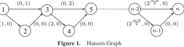
can be prohibitive in practice due to the size of the Pareto set which grows, in worst case, exponentially with the number of nodes. This can easily be shown by considering the family of instances intro-duced in [4]: 2 1 3 5 4 (2n2-3,0) (1, 0) n n-1 n-2 (0, 0) (2n2-3,0) (0, 0) (0, 2) (2, 0) (0, 0) (0, 1)
Figure 1. Hansen Graph
In the graph of Figure 1, we have an odd number of nodesn and 2n−1
2 distinct paths from node 1 to noden, leading to 2 n−1 2 distinct points(v1(k), v2(k)) = (k, 2 n−1 2 − 1 − k), k ∈ {0, . . . , 2 n−1 2 − 1}
in the space of criteria. By construction, these points are on the same line (they all satisfyv1(k)+v2(k) = 2
n−1
2 −1) orthogonal to vector (1, 1); therefore, they are all Pareto optimal. Although pathological,
such instances show that the determination of the Pareto set might reveal intractable in practice on large size instances. Numerical tests presented in Section 4 will confirm this point.
Moreover, even when the size of Pareto set is “reasonable”, the great majority of its elements do not provide interesting compromise solutions in practice. For instance, as soon as the criteria are conflict-ing, which is frequent in practice (e.g. cost vs quality, efficiency vs energy consumption), a path reaching the optimal value with respect to one criterion is often bad with respect to the other criteria. Such a path would not be a good compromise solution, yet it is a Pareto optimal solution. For this reason, it is worth defining more precisely the type of compromise sought in the Pareto set, so as then to focus the search on that type of compromise solution.
2.2
Looking for compromise solutions
A natural attitude to characterize good compromise solutions within the Pareto set is to define a scalarizing function:s : Nq
→ R in such
a way that the comparison of two pathsP and P′
represented by per-formance vectorsp and p′
reduces to the comparison of scalarss(p)
ands′
(p). In this respect, one might think that resorting to linear
scalarization of type:s1(p, ω) = Pi∈Qωipiwhereω is a strictly
positive weighting vector, is appropriate. Indeed, on the one hand, the path minimizings1(p, ω) over P(s, Γ) can easily be obtained.
It is sufficient to scalarize the problem by considering the valuation
w : A → R derived from v by setting w(a) = s1(v(a), ω) and
to applyA∗
with valuationw. On the other hand, weighted sum is
often seen as a natural aggregator to identify good compromise so-lutions. Although the first argument (procedural) is perfectly correct, the second is not valid on a non-convex set (which is the case here). The point is that minimizings1over the set of solution paths can only
reach supported solutions, i.e. those P-non-dominated solutions lying on the boundary of the convex hull of the points representing feasible solution-paths in the space of criteria. Hence there might exist fea-sible paths achieving a very well-balanced compromise solution that cannot be obtained by optimizings1(p, ω), whatever the choice of
the weighting vectorω. This problem, well known in multiobjective
optimization, is illustrated by Example 1.
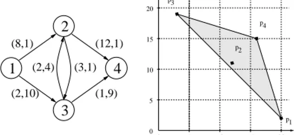
Example 1 Consider the bicriteria problem illustrated in Figure 2. In this graph, we have 4 paths from 1 (source node) to 4 (goal node):P1 = h1, 2, 4i , P2 = h1, 2, 3, 4i, P3 = h1, 3, 4i and P4 =
h1, 3, 2, 4i with v(p1) = (20, 2), v(p2) = (12, 11), v(p3) = (3, 19)
The graph to the right in Figure 2 represents the image of these solution-paths in the space of criteria. However we haves1(p1, ω) =
20ω1+ 2ω2,s1(p2, ω) = 12ω1+ 11ω2,s1(p3, ω) = 3ω1+ 19ω2
ands1(p4, ω) = 16ω1+15ω2. Sinces1is to be minimized,P1is
op-timal whenω1< ω2,P3is the optimal solution-path whenω2< ω1
and bothP1andP3are optimal whenω1= ω2. We can notice that
P2andP4cannot be optimal, whatever the choice ofω1andω2.
Al-though this is quite justified forP4which is P-dominated byP2this
is problematic forP2which is clearly the best compromise solution
path in this example. This is due to the fact thatP2lies inside the
convex hull of solutions (the grey triangle) and not on the boundary. p3 5 0 5 0 p2 p4 p1 20 15 10 10 15 20 (2,10) (12,1) (1,9) (8,1)
3
1
2
4
(3,1) (2,4)Figure 2. A bicriteria problem and its representation in the space of criteria
A better way of defining the notion of compromise solution for a solution-path P is to consider the distance between p = v(P )
and a prescribed reference vectorr (representing ideal performances,
or DM’s aspirations levels). This leads to formulate the following scalarizing function:
s(p, r, ω) =k ω.(p − r) k∞= maxi∈Q{ωi|pi− ri|}
in whichω is a weighting vector. The choice of Tchebycheff norm
focus on the worst component and therefore guarantees that only fea-sible solutions close to reference point r on every component will
receive a good score. This promotes well-balanced solutions. It also implies that iso-preference curves of types(x, r, ω) = k, for fixed r, ω and k, perfectly match P-dominance cones, which implies two
important properties on any subsetX ⊆ Nq(see [15]):
P1. If∀i ∈ Q, ωi > 0, then all solutions x minimizing s(x, r, ω)
over the setX of feasible cost vectors belongs to WND(X).
More-over at least one of these solutions belongs toND(X).
P2. Ifr ⋗ α then for all x ∈ ND(X) there exist strictly positive
weightsωi, i ∈ Q such that x is the unique solution minimizing
s(x, r, ω) over X.
Property P1 shows that minimizings yields well-balanced Pareto
optima located in the set N D(X) ∩ S(X) 6= ∅ where S(X) = arg minx∈Xs(x, r, ω). Property P2 shows that any type of
compro-mise solution can be obtained within the Pareto set, with the appro-priate choice of parametersr and ω. This second property explains
whys, as a scalarizing function, is preferred to s1in multiobjective
optimization on non-convex sets [15, 12].
We define normalization weights as followsωi = δi/(βi− αi),
for alli ∈ Q where [αi, βi] represents the range of possible values
for criterioni in the subarea of interest. Optimizing s generates a
weakly non-dominated path as close as possible to reference pointr
for the weighted Tchebycheff metric. Weights used in the metric can possibly be modified via coefficientsδiso as to give more importance
to some criteria. Functions induces a new dominance relation ≻son
Nq, defined byx ≻
sy ⇔ s(x, r, ω) < s(y, r, ω) which means that
x is a better compromise than y.
As mentionned in the introduction, compromise search can be seen as an interactive process. Initial parameters of functions are initially
chosen so as to focus on the center of the Pareto set but are dedicated
to evolve during the interactive exploration using standard updating techniques [12]. To save space, we now concentrate on the main tech-nical difficulty: the fast generation on the s-optimal path at a given step. This leads to the compromise search problem.
2.3
The compromise search problem
Compromise Search Problem. We want to determine all
P-non-dominateds-optimal feasible cost-vectors (i.e. N D(X)∩S(X) with X = {v(P ), P ∈ P(s, Γ)}) and the associated solution-paths.
Coming back to Example 1, withr = (0, 0) and ω = (1, 1)
we get:s(p1, r, ω) = 20, s(p2, r, ω) = 12, s(p3, r, ω) = 19 and
s(p4, r, ω) = 16. Hence the preferred compromise according to
≻s isP2 with cost-vector p2 = (12, 11) which seems quite
nat-ural here. Moreover, sub-paths from node 1 to node 3 are P with
costp = (11, 2) and P′
withp′ = (2, 10). Since p′
≻s p the
locally best compromise-path at node 3 isP′
. However, append-ing pathP′′ = h3, 4i with cost p′′ = (1, 9) to P and P′ respec-tively yieldsp + p′′ = (12, 11) and p′ + p′′ = (3, 19), so that p′ + p′′ ≺s p + p ′′
, a preference reversal. Notice that the optimal pathP2= P ∪ P′′would be lost during the search ifP is pruned at
node 3 due toP′
. Although the dominance relation≻sis much more
discriminating than P-dominance≻, which should improve pruning
possibilities and fasten the search, this example shows that the de-termination ofs-optimal solutions presents a new difficulty: we
can-not construct as-optimal path from s-optimal sub-paths. In other
words, the Bellman principle [1] does not hold. Moreover, the com-promise search problem is NP-hard. This can easily be derived from a result of Yu and Yang in [16] which proves that the Robust Devi-ation Shortest Path problem (RDSP for short) is NP-hard. In RDSP the goal is indeed to determine solution-paths minimizing function:
s(p, r) = maxi∈Q{|pi− ri|}. Optimizing our function s(p, r, ω)
with equal weightsωi, i = 1, . . . , q clearly reduces to RDSP.
3
ALGORITHMS
Knowing that solutions of the compromise search problem lie in the Pareto set, we first recall how Pareto-optimal paths are generated by MOA∗
algorithm.
3.1
Using MOA
∗for compromise search
Algorithm MOA∗
is a heuristic search algorithm generating all effi-cient paths ofG. It relies on the same foundations than A∗
, adapted to the field of vector-valued evaluation. In particular, the Bellman prin-ciple holds: anys-to-k subpath of a P-non-dominated solution-path,
is P-non-dominated inP(s, k). Hence, the algorithm constructs
in-crementally the P-non-dominated solution-paths from Pareto optimal subpaths. Let us briefly recall some essential features of MOA∗
(for more details, see [13]).
In a graph valued by cost-vectors, there possibly exists several P-non-dominated paths to reach a given node. Hence, at each de-tected noden, one stores a set G(n) of cost-vectors g(n)
corre-sponding to the valuations of P-non-dominated paths, among the set of already detected path arriving inn. Thus, G(n) is an
approxima-tion of the setG∗
(n) of all P-non-dominated cost vectors of paths
inP(s, n). Moreover, the algorithm uses a vector-valued heuristic.
Since a path arriving at noden can be continued with different
in-comparable subpaths to reachΓ, a set H(n) of heuristic cost-vectors h(n) is assigned to each node n. Thus, H(n) is an approximation
ofH∗
(n), the set of all P-non-dominated cost vectors of paths in P(n, Γ). As in A∗
, already detected nodes of the graph are par-titioned, at any step of the search, in two sets called OPEN (non-expanded nodes) and CLOSED (already (non-expanded nodes able to be expanded again). During the search, for any open noden, the set F (n) = ND({g(n) + h(n) : g(n) ∈ G(n), h(n) ∈ H(n)}) is
com-puted from all possible combinationsf (n) = g(n) + h(n). Such
vectors are called the labels of node n. Thus F (n) is a set of
la-bels (vectors) approximating the setF∗
(n) of all P-non-dominated
cost-vectors containing noden.
The principle of the search is, at the current step, to expand a node
n in OPEN such that F (n) contains at least one P-non-dominated
label among the labels of open nodes. The process is kept running until all open labels are either P-dominated by another label at the same node or by a vector solution-path already detected. It ensures to generate all efficient paths inP(s, n) provided heuristic H is
ad-missible, i.e.∀n ∈ N, ∀h∗
∈ H∗
(n), ∃h ∈ H(n) s.t. h ≻ h∗
. Knowing thats-optimal solutions are also P-non-dominated
solu-tions, the best compromise solution-path with respect to the Tcheby-cheff criterions should be sought within the Pareto set. Hence, a
straightforward way of determining best compromise solutions is 1) use MOA∗
to generate the Pareto set, and 2) determine thes-optimal
solutions in the output of MOA∗
. Such a two-stages procedure should not be very efficient in practice due to the size of the Pareto set. For this reason, we introduce now two algorithms aiming at directly fo-cusing on good compromise solutions.
3.2
BCA
∗BCA∗
is a variant of MOA∗
aiming at finding a best compromise path, i.e. a solution-pathP minimizing s(v(P ), r, ω) over P(s, Γ)
for a predefinedr and ω. The basic principle is to work on
P-non-dominated sub-paths while managing a current upper-bound λ to
store the values(v(P ), r, ω) of the best compromise path P among
already detected paths.
A preliminary stage consists of performingq monodimensionnal
optimizations (one per criterion) withA∗
so as to get one optimal pathPifor each criterioni ∈ Q. If pi = v(Pi) for all i, the ideal
point α is given by: αi = piifor alli ∈ Q. The nadir point β is
difficult to find in practice because the Pareto set is not known [3]. For this reason we use a classical approximation obtained by setting:
βi = maxj∈Qpijfor alli ∈ Q, whichs allows to compute weights
ωi = δi/(βi− αi), i ∈ Q. Then the choice of a given reference
pointr specifying the target in the space of criteria completely
de-fines functions (by default choose r close to α, see property P2).
Then the value ofλ is initialized to λ0= min{s(pi), i ∈ Q}. Hence
the main features of BCA∗
are:
Output: the best compromise solution-paths according tos. Principle: as in [9], we expand labels (attached to subpaths) rather
than nodes. We distinguish glabels (without heuristic h) from f
-labels (those used in MOA∗
). The search is totally ordered by func-tions. Thus, for any open node n and any f -label in F (n) we
com-pute the score s(f (n)) and we expand one of the f-labels having
minimal score (the more promising compromise subpath).
Pruning: We use the following pruning rules: 1) at noden, we prune
any subpath with a g-label P-dominated by the g-label of another
subpath at the same noden. 2) we prune any subpath P at node n if
itsf -label f (n) is such that s(f (n)) > λ. This second rule allows an
early elimination of subpaths that cannot lead to the best compromise solutions. These rules are justified by the following proposition:
Proposition 1 ∀x, y ∈ Nq, x ≻ y ⇒ x ≻
s y. Moreover ∀x, y, z ∈
Nq,(x ≻
sy and y ≻ z) ⇒ x ≻sz.
Indeed, during the search, if a subpathP is P-dominated by
an-other subpath P′
at the same node n according to g-labels, any
extension ofP will be P-dominated by the same extension of P′
, and therefore s−dominated. Similarly, if a subpath P is such that f (v(P )) > λ = v(P∗
), P∗
being the best already detected solution-path, any extension ofP will also be s−dominated by P∗
.
Heuristics: we use any admissible heuristic that can be used in
MOA∗
. In particular, we do not need to require that for all nodes
n, H(n) contains at least one perfectly informed label, as it is done
to justifyU∗
[14].
Stopping condition: Each time a node ofΓ is reached with a new
pathP such that λ > s(v(p), r, ω), the bound λ is updated. The
algorithm is kept running until all open labels of typef (n) satisfy s(f (n)) > λ. Termination obviously derives from the termination
of MOA∗
. In worst case, BCA∗
performs the same enumeration as MOA∗
and finds the best compromise at the last step. Of course, in average, BCA∗
stops much earlier, as we shall see in the next section.
3.3
kA
∗The second algorithm, called kA∗
, relies on the enumeration ofk
best paths in a scalarized versionG′
of the multiobjective graphG.
Scalarization is obtained by considering the valuationw : A → R
derived fromv by setting w(a) = s1(v(a), ω) for all a ∈ A (linear
aggregation of criteria). Hence, any pathP initially valued by a
vec-torp ∈ Nq
is now valued by the scalar costw(P ) = s1(p, ω).
Actu-ally, using functions1is interesting even if its optimization does not
provide directly compromise solutions. The point is thats-optimal
solutions often achieve a good performance according tos1. Hence,
we propose to enumerate solution-paths inG by increasing order of s1, which amounts to enumerating solution-paths inG′by increasing
order ofw. During enumeration, the s-optimal path can be identified
thanks to the following proposition:
Proposition 2 ∀x, y ∈ Nq ,s1(y, ω) > s1(¯xω, ω) =⇒ s(y, r, ω) > s(x, r, ω) with ∀i ∈ Q, ¯xωi= ri+ 1 ωis(x, r, ω). Indeed, denotingP1, . . . , Pj
the first solution-paths in the enumer-ation, we haves1(p1, ω) ≤ . . . ≤ s1(pj, ω). Suppose that Pj is
the first of these paths satisfying s1(pj, ω) > s1(¯p∗ω, ω) where
p∗
= arg mini=1,...,js(pi, r, ω) is the cost of the current best path
P∗
, then proposition 2 implies that all forthcoming pathsPk, k > j
in the enumeration will satisfys(pk, r, ω) > s(p∗
, r, ω). Therefore P∗
is the best compromise solution-path with respect tos and we
can stop the enumeration. Hence the main features of kA∗
are:
Output: the best compromise solutions according tos.
Principle: The ordered enumeration of best paths according to s1
can easily be performed using a modified version ofA∗
that works on labels attached to paths instead of labels attached to nodes. More precisely, to any detected pathPi
s,n froms to n, we assign a
la-bel of typefi(n) = gi(n) + h(n) where gi(n) = w(Pi s,n) and
h(n) is the value of an admissible heuristic function at node n
(∀n ∈ N, h(n) ≤ h∗
(n) where h∗
(n) is the cost of the optimal path
inP(n, Γ)). Hence, we have as many labels at a given node n as
de-tected sub-paths froms to n. Here G(n) (resp. F (n)) denotes the set
ofg-labels (resp. f -labels) of detected sub-paths from s to n. So we
haveF (n) = {fi(n) = gi(n) + h(n), gi(n) ∈ G(n)}. At node n,
f(i)(n) denotes the ith
smallest value inF (n). At the current step,
we expand the labelf(1)(n) = min
t∈OP ENf(1)(t). Since f(1)(n)
another label of F (n) before the best solution-path corresponding
tof(1)(n) is developped. Therefore n is put in CLOSED. If n is a
goal node then thekthpathPkis found. In this case, for all nodest
alongPk
, we delete the labelf(1)(t) in F (t). In order to expand the
newf(1)-label of these nodes, we set all these nodest in OPEN. If
s(pk, r, ω) < s(p∗
, r, ω) (where p∗
is the best detected cost vector) and we setP∗
← Pk
.
Heuristics: any type of admissible scalar-valued heuristic, e.g., any h derived by linear scalarization of an admissible heuristic used in
MOA∗
sinces1is strictly monotonic with respect to P-dominance.
Stopping condition: thanks to proposition 2, path enumeration
is kept running until a solution-path Pk such that s
1(pk, ω) >
s1(¯p∗ω, ω) (where P ∗
is the best current path) is detected.
4
EXPERIMENTATIONS
Numerical experiments have been performed to compare the three solutions discussed in the paper for compromise search: MOA∗
(completed with the determination of s-optimal solutions in the Pareto-set) BCA∗
and kA∗
. The computational experiments were carried out with a Pentium IV with 2.5GHz processor. Algorithms were implemented in C++. We first present result on randomly gen-erated instances and then on pathological instances.
Randomly generated graphs. We relate here results obtained by
executing algorithms on randomly generated graphs. The number of nodes in these graphs varies from 200 to 1,000 and the number of arcs from 7,500 (for 200 nodes) to 200,000 (for 1,000 nodes). Cost vec-tors are randomly determined for each arc. In practice, good admis-sible heuristics depend on the application domain. Independently of the context, we can generate admissible heuristic for tests, by setting
H(n) = µ(n)H∗
(n) for vector valued optimization, where µ(n)
is a randomly generated number within the unit interval at noden.
For kA∗
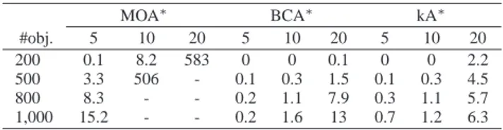
, the heuristic is obtained from the previous one by linear scalarization. Table 1 presents the average execution times (in sec-ond) obtained by the three algorithms for different class differing by the size of instances (number of nodes, number of criteria). In each class, average times are computed over 50 different instances. Sym-bol “-” means that execution time exceeds one hour.
Table 1. Execution time (s) on Random Graphs MOA∗ BCA∗ kA∗ #obj. 5 10 20 5 10 20 5 10 20 200 0.1 8.2 583 0 0 0.1 0 0 2.2 500 3.3 506 - 0.1 0.3 1.5 0.1 0.3 4.5 800 8.3 - - 0.2 1.1 7.9 0.3 1.1 5.7 1,000 15.2 - - 0.2 1.6 13 0.7 1.2 6.3
These results show that BCA∗
and kA∗
determine thes-optimal
so-lution paths significantly faster than MOA∗
. Indeed, for a graph con-taining more than 500 nodes and 10 criteria, MOA∗
requires more than one hour to generate thes-optimal solutions whereas BCA∗
and kA∗
need some seconds. We see that the sophistication proposed in BCA∗
really speed-up the search of the best compromise solutions. Moreover, we can notice that BCA∗
is slightly faster than kA∗
when the size of the graph is small, but kA∗
outperforms BCA∗
as the size of the instance increases.
Hansen graphs. Now, algorithms are compared on Hansen graphs
(Figure 1). All feasible paths in this family of graphs are P-non-dominated. Then MOA∗
generates all solution-paths. Since for any pathP in Hansen’s family, we have s1(¯p∗ω, ω) > s1(p, ω) (where
P∗
is the best compromise path), kA∗
generates all feasible paths too. Table 2 summarizes execution times obtained on these graphs.
Table 2. Execution time (s) on Hansen Graphs #nodes MOA∗ BCA∗ kA∗
21 0.01 0 0 25 3.1 1.1 0 29 70.2 25.5 0.15 33 1147 427.9 0.61
These results show the advantage of resorting to a scalarized ver-sion of the graph. Indeed kA∗
reveals very efficient when the number of P-non-dominated paths is important, because scalarization avoids numerous Pareto-dominance tests.
5
CONCLUSION
We have introduced two admissible algorithms to determine the best compromise paths in multivalued state space graphs. Although they produce the same solutions, BCA∗
is based on a focused exploration of the Pareto-set in a multiobjective space while kA∗
solves the same problem by working on a scalarized version of the graph. As ex-pected, tests confirm that the two approaches are much more efficient than explicit enumeration of the Pareto set to solve the compromise search problem. An advantage of the approach used in kA∗
is that it applies to any other multiobjective problem, provided the scalar ver-sion can be solved efficiently. Both algorithms perform a fast genera-tion of the best current compromise solugenera-tion and could be incorporate into an interactive exploration procedure of the Pareto set.
REFERENCES
[1] R. Bellman, Dynamic Programming, Princeton University Press, 1957. [2] P. Dasgupta, P.P. Chakrabarti, and S.C. DeSarkar, ‘Utility of pathmax in partial order heuristic search’, J. of algorithms, 55, 317–322, (1995). [3] M. Ehrgott and D. Tenfelde-Podehl, ‘Computation of ideal and nadir values and implications for their use in mcdm methods’, European
Journal of Operational Research, 151(1), 119–139, (2003).
[4] P. Hansen, ‘Bicriterion path problems’, in Multiple Criteria Decision
Making: Theory and Applications, LNEMS 177, eds., G. Fandel and
T. Gal, 109–127, Springer-Verlag, Berlin, (1980).
[5] P. E. Hart, N. J. Nilsson, and B. Raphael, ‘A formal basis for the heuris-tic determination of minimum cost paths’, IEEE Trans. Syst. and Cyb.,
SSC-4 (2), 100–107, (1968).
[6] U. Junker, ‘Preference-based search and multi-criteria optimization.’, in AAAI/IAAI, pp. 34–40, (2002).
[7] P. Kouvelis and G. Yu, Robust discrete optimization and its
applica-tions, Kluwer Academic Publisher, 1997.
[8] B. Logan and N. Alechina, ‘A∗with bounded costs’, in Proceedings of
AAAI-98. AAAI Press/MIT Press, (1998).
[9] L. Mandow and J.L. Prez de la Cruz, ‘A new approach to multiobjec-tive a∗search’, in Proceedings of IJCAI-05, pp. 218–223. Professional
Book Center, (2005).
[10] P. Perny and O. Spanjaard, ‘Preference-based search in state space graphs’, in Proceedings of AAAI-02, pp. 751–756, (2002).
[11] P. Perny and O. Spanjaard, ‘An axiomatic approach to robustness in search problems with multiple scenarios’, in Proceedings of UAI, pp. 469–476, Acapulco, Mexico, (8 2003).
[12] R.E. Steuer and E.-U. Choo, ‘An interactive weighted Tchebycheff pro-cedure for multiple objective programming’, Mathematical
Program-ming, 26, 326–344, (1983).
[13] B.S. Stewart and C.C. White III, ‘MultiobjectiveA*’, Journal of the
Association for Computing Machinery, 38(4), 775–814, (1991).
[14] C.C. White, B.S. Stewart, and R.L. Carraway, ‘Multiobjective, preference-based search in acyclic OR-graphs’, European Journal of
Operational Research, 56, 357–363, (1992).
[15] A.P. Wierzbicki, ‘On the completeness and constructiveness of para-metric characterizations to vector optimization problems’, OR
Spek-trum, 8, 73–87, (1986).
[16] G. Yu and J. Yang, ‘On the robust shortest path problem’, Comput.