HAL Id: tel-01138336
https://pastel.archives-ouvertes.fr/tel-01138336
Submitted on 1 Apr 2015
HAL is a multi-disciplinary open access
archive for the deposit and dissemination of
sci-entific research documents, whether they are
pub-lished or not. The documents may come from
teaching and research institutions in France or
L’archive ouverte pluridisciplinaire HAL, est
destinée au dépôt et à la diffusion de documents
scientifiques de niveau recherche, publiés ou non,
émanant des établissements d’enseignement et de
recherche français ou étrangers, des laboratoires
Connected component tree construction for embedded
systems
Petr Matas
To cite this version:
Petr Matas. Connected component tree construction for embedded systems. Computer science.
Uni-versité Paris-Est, 2014. English. �NNT : 2014PEST1116�. �tel-01138336�
University of West Bohemia
Faculty of Electrical Engineering
and
Université Paris-Est
École Doctorale MSTIC
THESIS
to obtain the Doctor of Philosophy degree of the University of West Bohemia
and Université Paris-Est with specialization in Computer Science
Connected Component Tree
Construction for Embedded Systems
Petr Matas
presented on 30 June 2014
Composition of the Examination Committee:
Serge WEBER
Professor, University of Lorraine
Reviewer
Petr MATULA
Assoc. professor, Masaryk University Brno
Reviewer
Mohamed AKIL
Professor, ESIEE Paris
Director
Vjačeslav GEORGIEV
Assoc. professor, University of West Bohemia
Director
Václav MATOUŠEK
Professor, University of West Bohemia
Chairman
Abstract
The aim of this work is to enable construction of embedded digital image processing systems, which are both flexible and powerful. The thesis proposal explores the possibility of using an image representation called connected component tree (CCT) as the basis for implementation of the entire image processing chain. This is possible, because the CCT is both simple and general, as CCT-based implementations of operators spanning from filtering to segmentation and recognition exist. A typical CCT-based image processing chain consists of CCT construction from an input image, a cascade of CCT transformations, which implement the individual operators, and image restitution, which generates the output image from the modified CCT. The most time-demanding step is the CCT construction and this work focuses on it.
It introduces the CCT and its possible representations in computer memory, shows some of its applications and analyzes existing CCT construction algorithms. A new parallel CCT construction algorithm producing the parent point tree representation of the CCT is proposed. The algorithm is suitable for an embedded system implementation due to its low memory requirements. The algorithm consists of many building and merging tasks. A building task constructs the CCT of a single image line, which is treated as a one-dimensional signal. Merging tasks fuse the CCTs together. Three different task scheduling strategies are developed and evaluated. Performance of the algorithm is evaluated on multiple parallel computers. A throughput 83 Mpx/s at speedup 13.3 is achieved on a 16-core machine with Opteron 885 CPUs.
Next, the new algorithm is further adapted for hardware implementation and implemented as a new parallel hardware architecture. The architecture contains 16 basic blocks, each dedicated to processing of an image partition and consisting of execution units and memory. A special interconnection switch is designed to allow some executions units to access memory in other basic blocks. The algorithm requires this for the final merging of the CCTs constructed by different basic blocks together. The architecture is implemented in VHDL and its functional simulation shows performance 145 Mpx/s at clock frequency 120 MHz.
Keywords
connected component tree, parent point tree, construction, graph, attributes, building, merging, parallel, concurrent, embedded, algorithm, scheduling, image processing, hardware, VHDL, FPGA
Résumé
L’objectif du travail présenté dans cette thèse est de proposer un avancement dans la construction des systèmes embarqués de traitement d’images numériques, flexibles et puissants. La proposition est d’explorer l’utilisation d’une représentation d’image particulière appelée « arbre des composantes connexes » (connected component tree – CCT) en tant que base pour la mise en œuvre de l’ensemble de la chaîne de traitement d’image. Cela est possible parce que la représentation par CCT est à la fois formelle et générale. De plus, les opérateurs déjà existants et basés sur CCT recouvrent tous les domaines de traitement d’image : du filtrage de base, passant par la segmentation jusqu’à la reconnaissance des objets. Une chaîne de traitement basée sur la représentation d’image par CCT est typiquement composée d’une cascade de transformations de CCT où chaque transformation représente un opérateur individuel. A la fin, une restitution d’image pour visualiser les résultats est nécessaire. Dans cette chaîne typique, c’est la construction du CCT qui représente la tâche nécessitant le plus de temps de calcul et de ressources matérielles. C’est pour cette raison que ce travail se concentre sur la problématique de la construction rapide de CCT.
Dans ce manuscrit, nous introduisons le CCT et ses représentations possibles dans la mémoire de l’ordinateur. Nous présentons une partie de ses applications et analysons les algorithmes existants de sa construction. Par la suite, nous proposons un nouvel algorithme de construction parallèle de CCT qui produit le « parent point tree » représentation de CCT. L’algorithme est conçu pour les systèmes embarqués, ainsi notre effort vise la minimisation de la mémoire occupée. L’algorithme en lui-même se compose d’un grand nombre de tâches de la « construction » et de la « fusion ». Une tâche de construction construit le CCT d’une seule ligne d’image, donc d’un signal à une dimension. Les tâches de fusion construisent progressivement le CCT de l’ensemble. Pour optimiser la gestion des ressources de calcul, trois différentes stratégies d’ordonnancement des tâches sont développées et évaluées. Également, les performances des implantations de l’algorithme sont évaluées sur plusieurs ordinateurs parallèles. Un débit de 83 Mpx/s pour une accélération de 13,3 est réalisé sur une machine 16-core avec Opteron 885 processeurs.
Les résultats obtenus nous ont encouragés pour procéder à une mise en œuvre d’une nouvelle implantation matérielle parallèle de l’algorithme. L’architecture proposée contient 16 blocs de base, chacun dédié à la transformation d’une partie de l’image et comprenant des unités de calcul et la mémoire. Un système spécial d’interconnexions est conçu pour permettre à certaines unités de calcul d’accéder à la mémoire partagée dans d’autres blocs de base. Ceci est nécessaire pour la fusion des CCT partiels. L’architecture a été implantée en VHDL et sa simulation fonctionnelle permet d’estimer une performance de 145 Mpx/s à fréquence d’horloge de 120 MHz.
Mots-clés
arbre des composantes connexes, parent point tree, construction, graphe, attributs, fusion, calculs parallèles, système embarqué, algorithme, programmation, traitement d’image, VHDL, FPGA
Anotace
Cílem této práce je umožnit konstrukci vestavěných systémů pro zpracování digitalizovaného obrazu, které jsou zároveň flexibilní a výkonné. Zkoumá se možnost použití reprezentace snímku zvané strom souvislých
komponent (connected component tree, CCT) jako základu pro implementaci celého řetězce pro zpracování
obrazu. Toto je možné, protože CCT je zároveň jednoduchý i obecný. Existují totiž na CCT založené implementace operátorů od filtrování až po segmentaci a rozpoznávání. Typický řetězec zpracování obrazu založený na CCT sestává z konstrukce CCT ze vstupního snímku, kaskády transformací CCT, které implementují jednotlivé operátory, a restituce obrazu, která generuje výstupní snímek z modifikovaného CCT. Časově nejnáročnějším krokem je konstrukce CCT a tato práce se na ni zaměřuje.
Práce představuje CCT a jeho možné reprezentace v počítačové paměti, ukazuje některé jeho aplikace a ana-lyzuje existující algoritmy konstrukce CCT. Je navržen nový paralelní algoritmus konstrukce CCT, jehož výstupem je reprezentace CCT zvaná parent point tree. Tento algoritmus je vhodný k implementaci ve vestavěných systémech díky malým paměťovým nárokům. Algoritmus se skládá z mnoha úloh stavění a slučování. Z jednoho řádku snímku, se kterým se zachází jako s jednorozměrným signálem, stavění vytvoří CCT a slučování spojují tyto CCT dohromady. Tři různé strategie plánování úloh jsou vyvinuty a zhodnoceny. Výkonnost algoritmu je otestována na několika paralelních počítačích. Na 16jádrovém stroji s procesory Opteron 885 je dosaženo propustnosti 83 Mpx/s při 13,3násobném zrychlení paralelizací. Následně je algoritmus dále adaptován pro hardwarovou implementaci a implementován jako nová paralelní hardwarová architektura. Ta obsahuje 16 základních bloků, z nichž každý zpracovává část snímku a skládá se z výkonných jednotek a pamětí. Je navržen speciální propojovací přepínač, aby některé výkonné jednotky mohly přistupovat k paměti v ostatních základních blocích. Algoritmus toto vyžaduje pro závěrečné slučování CCT vytvořených různými základními bloky dohromady. Architektura je implementována ve VHDL a její funkční simulace dává výkonnost 145 Mpx/s při frekvenci hodin 120 MHz.
Klíčová slova
strom souvislých komponent, parent point tree, konstrukce, graf, atributy, stavění, slučování, paralelní, konkurentní, zapouzdřený, vestavěný, algoritmus, plánování, zpracování obrazu, hardware, VHDL, FPGA
Contents
Abstract 2 Résumé 3 Anotace 4 List of figures 7 List of tables 9 List of algorithms 9 Acknowledgements 10Abbreviations and symbols 11
1 Introduction 13
1.1 Embedded systems for vision . . . 13
1.2 Motivation for graph-based formalism . . . 14
2 Connected component tree and its applications 17 2.1 Mathematical background . . . 17
2.1.1 Digital image as a weighted graph . . . 17
2.1.2 Connected component tree (CCT) . . . 19
2.2 CCT representations . . . 21
2.3 Attributes . . . 23
2.4 Examples of applications . . . 28
2.4.1 Attribute filters . . . 28
2.4.2 Segmentation 1: Detection of maximally stable extremal regions . . . 30
2.4.3 Segmentation 2: Topological watershed . . . 32
2.4.4 Segmentation without CCT: Inter-pixel watershed . . . 33
2.5 Conclusions . . . 34
3 Algorithm architecture matching 36 3.1 Discussion, evaluation and comparison of existing CCT construction algorithms . . . 36
3.1.1 CCT construction algorithm classes . . . 36
3.1.2 Flooding algorithm description . . . 37
3.1.3 Past parallelization efforts . . . 39
3.3 Parallel program performance assessment quantities . . . 42
3.3.1 Speedup . . . 42
3.3.2 Performance improvement . . . 42
3.3.3 Efficiency . . . 43
3.3.4 Hardware thread utilization . . . 43
3.3.5 Software thread utilization . . . 43
3.4 Conclusions . . . 44
4 Parallel implementation of CCT construction 45 4.1 New parallel algorithm description . . . 45
4.1.1 High-level description of the algorithm . . . 45
4.1.2 Build: 1D partial point tree construction . . . 47
4.1.3 Merging of partial point trees . . . 49
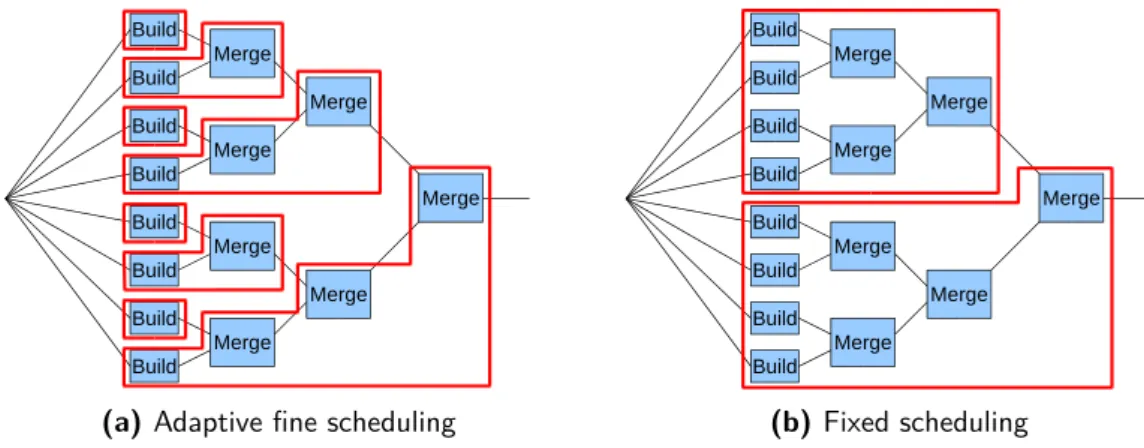
4.2 Scheduling strategies . . . 49
4.2.1 Inter-frame parallelism . . . 49
4.2.2 Intra-frame parallelism . . . 51
4.2.3 Strategy 1: Adaptive fine scheduling . . . 52
4.2.4 Strategy 2: Fixed scheduling . . . 54
4.2.5 Strategy 3: Adaptive coarse scheduling . . . 55
4.2.6 Theoretical comparison of the strategies . . . 55
4.3 Performance evaluation . . . 56
4.3.1 Time complexity and memory requirements . . . 56
4.3.2 Execution time measurement method . . . 56
4.3.3 Time measurement resolution assessment experiments . . . 57
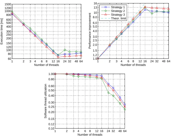
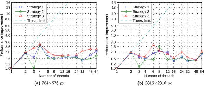
4.3.4 Results . . . 58
4.3.5 Discussion of the results . . . 58
4.3.6 Comparison of the scheduling strategies . . . 61
4.4 Conclusions . . . 61
5 Hardware architecture for CCT construction 63 5.1 Algorithm modifications for hardware implementation . . . 63
5.1.1 1D CCT construction algorithm . . . 64
5.1.2 Progressive CCT fusion algorithm . . . 66
5.1.3 Dataflow representation of overall CCT construction algorithm . . . 66
5.2 Original parallel hardware architecture description . . . 67
5.2.1 Overall architecture . . . 67
5.2.2 Build . . . 69
5.2.3 Merge . . . 70
5.2.4 Merging boundary line numbers generator . . . 72
5.2.5 Memory access network . . . 73
5.3 Scalability discussion . . . 75
5.4 Performance evaluation and implementation results . . . 76
6 Conclusions and perspectives 79
Publications 81
Bibliography 82
Appendix A Inter-pixel watershed algorithm 85
Appendix B Parallel CCT construction algorithm software implementation timings 87
List of figures
1.1 Questions to and actions of the example computer vision system . . . 14
1.2 Stages of a typical CCT-based application with relative execution times . . . 15
2.1 Undirected loopless graph examples . . . 18
2.2 Graph representation of an image . . . 19
2.3 Two possible descriptions of a binary image . . . 20
2.4 A connected component tree example . . . 21
2.5 The classic representation of the CCT . . . 22
2.6 The point tree . . . 22
2.7 The parent point tree and its storage in the array of parent pointers . . . 24
2.8 Illustration of the attribute Area on a 1D signal . . . 24
2.9 Illustrations of attributes Minimum, Maximum, and Range . . . 25
2.10 Illustrations of three definitions of the attribute Volume . . . 26
2.11 Different variants of attribute filters . . . 29
2.12 An attribute filtering example . . . 30
2.13 A maximally stable extremal regions example . . . 31
2.14 Topological watershed results demonstration . . . 33
3.1 Evolution of a software thread in time . . . 43
4.1 Output from the new parallel algorithm . . . 46
4.2 Data dependency graph of the new parallel algorithm . . . 46
4.3 Distribution of the Build and Merge operations among threads . . . 52
4.4 Meaning of the variable border (the merging boundary line number) . . . . 54
4.5 Timer evaluation results . . . 57
4.6 Timing results of the new algorithm on 16 cores . . . 59
5.1 CCT construction dataflow diagram . . . 66
5.2 Overall structure of the new CCT construction architecture . . . 67
5.3 1D CCT building unit RTL structure . . . 69
5.4 Build controller state transition diagram . . . 70
5.5 CCT merging unit RTL structure . . . 71
5.6 Merge controller state transition diagram . . . 71
5.7 TreeConnect 1 and 2 for 16 basic blocks . . . 73
5.8 TreeConnect 3 for 16 basic blocks . . . 73
5.9 Execution units’ utilization versus time (natural image) . . . 77
B.1 Input images used for measurements . . . 87
B.2 Goldhill (784×576, 8 bits) – Strategy 1 . . . 89
B.3 Goldhill (784×576, 8 bits) – Strategy 2 . . . 90
B.4 Goldhill (784×576, 8 bits) – Strategy 3 . . . 91
B.5 Goldhill (784×576, 8 bits) – 2 cores . . . 92
B.6 Goldhill (784×576, 8 bits) – 2 cores with hyper-threading . . . 93
B.7 Goldhill (784×576, 8 bits) – 4 cores . . . 94
B.8 Goldhill (784×576, 8 bits) – 16 cores . . . 95
B.9 Earth (2816×2816, 8 bits) – Strategy 1 . . . 96
B.10 Earth (2816×2816, 8 bits) – Strategy 2 . . . 97
B.11 Earth (2816×2816, 8 bits) – Strategy 3 . . . 98
B.12 Earth (2816×2816, 8 bits) – 2 cores . . . 99
B.13 Earth (2816×2816, 8 bits) – 2 cores with hyper-threading . . . 100
B.14 Earth (2816×2816, 8 bits) – 4 cores . . . 101
List of tables
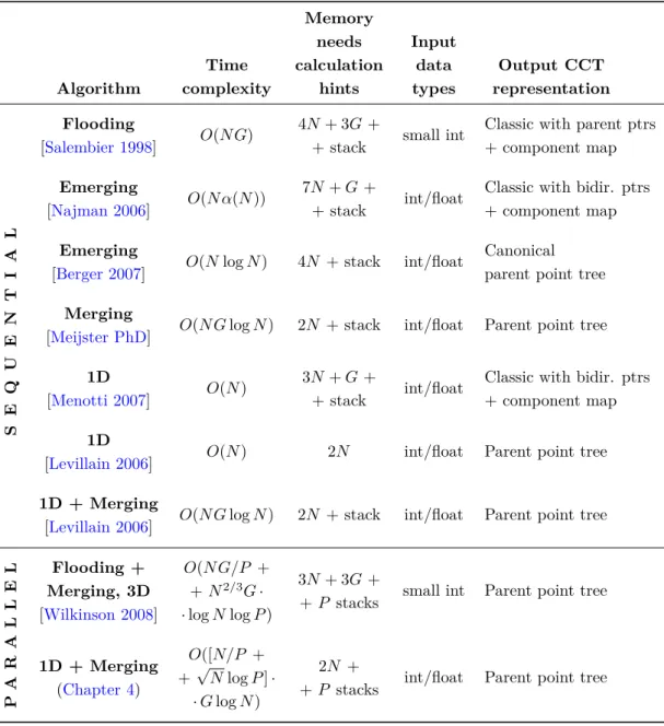
3.1 Complexity analysis of existing CCT construction algorithms . . . 40
4.1 Features of proposed scheduling strategies . . . 55
4.2 Cache miss count measurement results for the small image (784×576, 8 bits) . . . 59
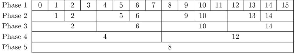
5.1 Which Merging units are active in each merging phase (for 16 basic blocks) . . . 68
5.2 Building algorithm and controller states . . . 70
5.3 Merging algorithm and controller states . . . 71
5.4 Merging boundary line numbers generator (4-bit) output sequence . . . 72
5.5 TreeConnect 1 and 2 multiplexers control . . . 74
5.6 Definition of addresses Si for TreeConnect 3 multiplexers control . . . 74
5.7 Functions d2, d4, d8, d16 . . . 75
5.8 Measured performance in FPGA . . . 76
5.9 FPGA resource utilization for a 512×512px image . . . 77
5.10 Performance comparison of CCT implementations . . . 77
B.1 Testing systems . . . 88
List of algorithms
2.1 Topological watershed definition . . . 322.2 Inter-pixel watershed definition . . . 34
3.1 CCT construction by flooding . . . 38
4.1 Parent point tree construction for a linear graph . . . 48
4.2 Merging of two parent point trees . . . 50
4.3 Concurrent parent point tree construction with Strategy 1: Adaptive fine scheduling . . . 53
5.1 Parent point tree construction for a linear graph. Adapted for a hardware implementation . . 64
5.2 Merging procedure connect adapted for a hardware implementation . . . 65
A.1 Inter-pixel watershed . . . 85
Acknowledgements
In the first place I want to thank God, who accompanied me from the start and showed me His mercy and unconditional love, even though I did not want to know Him yet. He brought to my life many people, which made completing this work possible:
My biggest thanks go to my thesis directors and consultants for their continuous guidance and help, i.e. to Vjačeslav Georgiev, who did not let me run away from the unfinished work, Mohamed Akil, who enabled me to see things from another points of view, Eva Dokládalová, who pushed me straight forward and taught me how research is done, and Martin Poupa, who opened the FPGA domain to me.
I appreciate the kind acceptance and support from the A3SI laboratory members. I owe a lot also to other people who were helping me and supporting me during my work: Harold Phelippeau, Václav Valenta,
Jan Bartovský, Imran Taj, Ramzi Mahmoudi, David Hnilica, Petr Dokládal, David Menotti, Milan Dlauhý, and others.
Thanks are also addressed to Joëlle Delers and Samuel from acc&ss Paris-Est (formerly BiCi – Bureau international des Chercheurs invités) for making my installation in France easy and fun. Additionally, my work would not have been possible without the generous financial support from the French government. The access to computing and storage facilities owned by parties and projects contributing to the
Meta-Centrum National Grid Infrastructure [MetaCentrum], provided under the program “Projects of Large Infrastructure for Research, Development, and Innovations" (LM2010005) is also acknowledged.
Special thanks belong to my parents and extended family members, who accompanied me on the dark parts of the path. Substantial strength to go ahead originated also from the members of the Christian
Abbreviations and symbols
1D, 2D, ... 1-dimensional, 2-dimensional, ...
C Connected component CCT Connected component tree
D Set of possible image sample values – image codomain
E Pixel neighborhood relation and mapping
f Image function fps Frames per second
G Graph representation of an image
G Number of grey levels of an image, G = |D|
H Height of an image in pixels
HT Hyper-Threading, the Intel’s implementation of SMT IPW Inter-pixel watershed
log x Logarithm of x (base is not specified) LSB Least significant bit
max S Maximum of the elements of the set S min S Minimum of the elements of the set S Mpx/s Megapixel per second
MSB Most significant bit
N Number of pixels of an image, N = |V |. For a 2D image, N = W · H N0 Set of non-negative integers {0, 1, 2, ...}
N1 Set of positive integers {1, 2, 3, ...}
O Big O notation. f (x) ∈ O(g(x)) means that up to a multiplicative constant, f (x) does not grow asymptotically faster than g(x) as x goes to infinity, i.e. ∃c ∈ R, x0 ∈ R : ∀x > x0 :
|f (x)| ≤ c · |g(x)|. For example, 2x ∈ O(x) and x ∈ O(x2)
Θ Big Theta notation. f (x) ∈ Θ(g(x)) means that up to a multiplicative constant, f (x) grows asymptotically as fast as g(x) as x goes to infinity, i.e. f (x) ∈ O(g(x)) ∧ g(x) ∈ O(f (x)) px Pixel, picture element, one sample of an iconic image of any dimension (1D, 2D, 3D, ...)
R Set of real numbers
R+ Set of positive real numbers
SMT Simultaneous multithreading, a technique allowing multiple hardware threads per processor core
TW Topological watershed
V Set of points of an image – image domain
W Width of an image in pixels Z Set of integers
P ∧ Q Logical conjunction of two predicates (P and Q)
P ∨ Q Logical disjunction of two predicates (P or Q)
P ⇒ Q Implication between two predicates (if P , then Q)
P ⇔ Q Equivalence of two predicates (P precisely if Q)
x ∈ S x is an element of the set S x /∈ S x is not contained in the set S
(a, b, c) Ordered n-tuple given as a list of its elements {a, b, c} Set given as a list of its elements
{x : P } Set of all elements x fulfilling the predicate P
{x ∈ S : P (x)} Shorthand for {x : x ∈ S ∧ P (x)}, i.e. the set of all elements x from the set S fulfilling the predicate P (x)
∅ Empty set
A ∩ B Intersection of the sets A and B
A ∪ B Union of the sets A and B S
i∈SAi Union of all sets Ai, where i ∈ S
P
i∈Sxi Sum of all values xi, where i ∈ S
A \ B Asymmetric difference of the sets A and B, i.e. the set {x ∈ A : x /∈ B}
A ⊂ B A is the subset of B, i.e. every element from A is contained also in B. Equality of the
sets A and B is allowed
A ⊆ B A is the subset of B. Equality of the two sets is explicitly allowed A ( B A is the subset of B, but they are not equal
|x| Absolute value of the number x |S| Number of elements in the set S
[S] The unique element of the single-element set S; undefined if |S| 6= 1 bxc Floor function, i.e. the biggest integer not greater than x
2S Power set, i.e. the set of all subsets, of the set S ∀x : P (x) For all x, the predicate P (x) is true
∃x : P (x) For at least one x, the predicate P (x) is true
f : V → D f is a function (mapping) from domain V to codomain D f (x) Value of the function f at point x
A × B Cartesian product of the sets A and B, i.e. the set {(x, y) : x ∈ A ∧ y ∈ B} ⊥ Nothing. For example, if C has no parent, then P arent(C) = ⊥
x ← y Assign value y to variable x
x++ Increment variable x by one and return its previous value
Chapter 1
Introduction
1.1
Embedded systems for vision
Nowadays, image sensors are becoming omnipresent and a huge amount of data is available from them. However, human capacity to handle these data is quite limited, and therefore majority of them has to be discarded without ever being processed. This is the opportunity for computer vision systems, which may extract the small amount of useful information contained in the data and sometimes even make decisions based on it and take actions without human intervention.
The computer vision systems are asked to give high performance and be flexible for a large variety of existing or possible applications. As an example, imagine just a small video surveillance system composed of five video cameras with a full-HD resolution (1920×1080 px, 24 bit/px, 25 fps) around a busy crossroad. Each second, such system produces over 6 Gb (gigabits) of data, which should enter a complex processing. This justifies the performance requirements. Next, let us imagine some of the many questions, which we may want to pose to this system, and the actions it could take. Some of them are in Figure 1.1, which demonstrates the flexibility requirements.
One of the global problems of the vision system design is how to achieve both high performance and flexibility simultaneously. It is because, a) many image-processing methods exist and each of them suits a different (usually small) subset of the applications, and b) each application requires cascades of multiple image-processing operators to produce the result.
If the high performance is achieved by an optimization effort, which means a kind of system specialization, it will (by definition) limit its flexibility. For example, a device optimized for FFT (Fast Fourier Transform) and similar computations is predestined for frequency domain image filtering and for image compression, but non-linear image processing operators and image segmentation may be quite inefficient with it.
Questions to the vision system:
• How many vehicles are standing in each lane? • What are the speeds of the moving vehicles? • What are the vehicles’ registration numbers? • Where and how many pedestrians are present? • Is there any damage on the public transport vehicles? • Is the crossroad obstructed?
• Is a traffic collision taking place?
• Is a fallen person lying in the field of view?
• Is a fight, assault or pocket-picking taking place? Who are the offenders?
• Has a given person crossed the field of view in a given time span? Which way did he go? • What is the state of the road surface?
• What is the weather?
• What animal species live at the site?
Actions of the vision system:
• Traffic lights timing • Traffic reporting • Fine a speeding driver
• Alert police about location of a stolen vehicle or searched person • Public transport dispatch
• Emergency services dispatch
Figure 1.1: Questions to and actions of the example computer vision system
1.2
Motivation for graph-based formalism
The image-processing operators may be usually classified into one of the following two categories: • Low-level (local processing) operators: pre-processing, filtering
• High-level (image analysis) operators: segmentation, pattern recognition, motion extraction. . .
Simultaneous optimization of algorithms from both categories is particularly difficult using classic approaches, because the two categories’ requirements are quite different from each other. Image-processing algorithms based on connected component tree (CCT) seem to be very promising from this point of view. They allow bridging the gap between low- and high-level processing elements. They have been used for image filtering [Salembier 1998, Wilkinson 2008], as well as the image analysis: motion extraction [Salembier 1998], wa-tershed segmentation [Couprie 2005,Najman 2006,Mattes 2000], pattern recognition in astronomical imag-ing [Berger 2007,Jalba 2004], microscopic image analysis [Cuisenaire 1999], video-surveillance applications [Piscaglia 1999], image registration [Mattes 1999], or data visualization [Chiang 2005].
CCT
80% of time
Input Image CCT Filtering Motion detection ... Output Image20% of time
Segmentation Image Restitution Tree Construction Tree Transformation Performance bottleneckFigure 1.2: Stages of a typical CCT-based application with relative execution times
Another perspective for treating the flexibility problem are the data structures used for image analysis, which may be roughly classified into four levels going from the lowest to the highest level of abstraction [Sonka 2008]:
• Iconic images are matrices containing original data about pixel brightness or results of the image pre-processing.
• Segmented images join parts of the image into regions, which are likely to belong to the same objects or their borders.
• Geometric representations describe and quantify the shapes of the image regions. • Relational models collect the information about relations among the objects in the image.
A flexible computer vision system will surely have to support data structures from all these four levels. The CCT is a unique data structure, which covers (at least partially) all of them: The iconic image is contained directly. Next, the CCT is composed of components – image regions – and the CCT can be therefore seen also as a segmented image. The component attributes allow characterization and quantification of many component properties including (but not limited to) the shape, which qualifies the CCT partly as a geometric representation. Finally, as components are organized into a hierarchic structure, the CCT is a simple relational model too.
Figure 1.2 shows typical stages of an application based on CCT. We can see another advantage of these methods: the processing is performed on the constructed CCT by graph transformation(s), and only one data structure is used from low-level to high-level processing.
On the other hand, the main bottleneck is the CCT construction, consuming about 80 % of the application execution time [Ngan 2011], which is penalizing for many practical applications. However, once the CCT has been constructed, the rest of the application executes quite fast. Therefore, this work focuses on acceleration of the CCT construction.
The key concept used by the CCT and the CCT-based algorithms is connectivity, i.e. existence of a contiguous path between two pixels of a given subset of the image domain. This is best described when we treat the image as a weighted graph, introduced inSection 2.1.1, which allows the CCT-based algorithms to be applied to images of any dimension (1D, 2D, 3D. . . ) and connectivity. The CCT itself is a graph too, as tree is a special graph. The graph representation is also the most easily understandable form to imagine how
a structure works and what to do to make it working in our way. Note that many other components of intelligent vision systems are organized around the graphs (for example databases, knowledge bases and environment models). Graphs are widely used not only in image processing, but also in other disciplines such as digital signal processing and economy.
Chapter 2
Connected component tree and its
appli-cations
As stated in the introductory chapter, the connected component tree (CCT) is a representation of digital images, which allows efficient implementations of many image-processing operators from image filtering through watershed segmentation to data visualization.
This chapter introduces the graph-based digital image representation, explains the CCT, and presents its memory representations and some application examples.
2.1
Mathematical background
This section defines the mathematical terms that will be used later on. The majority of the definitions are stated in pairs:
The definition using intuitive wording and allowing fast reading comes first.
The mathematically precise formal definition follows and is indented. Skipping it will not hamper general understanding, but this definition resolves any ambiguities, that the intuitive definition cannot easily avoid, and introduces the symbolic notation.
2.1.1
Digital image as a weighted graph
A graph is a mathematical representation of a set of objects where some of them are connected by links. The interconnected objects are called vertices and the links between them are called edges. Two examples are shown in Figure 2.1. Both are undirected loopless graphs. Such graphs will be used for digital image representation.
v
4v
5v
3v
6v
2v
1e
1e
2e
7e
6e
4e
3e
5(a) A general graph. The set of vertices V = {v1, . . . , v6},
the set of (undirected) edges E = {e1, . . . , e7}
(b) A linear graph
Figure 2.1: Undirected loopless graph examples
The undirected loopless graph is a pair G = (V, E), where • V is a finite set of vertices,
• E ⊂ V × V is a binary neighborhood relation (the set of edges), which is
– symmetric (ensures undirectedness): ∀x, y : (x, y) ∈ E ⇔ (y, x) ∈ E, – and anti-reflexive (ensures looplessness): ∀x : (x, x) 6∈ E
[Najman 2006,Wilkinson 2008].
An undirected edge notation {x, y} may be used as a shortcut for the pair of edges (x, y) and (y, x). The neighborhood relation E may be used also in the form of neighborhood mapping E : V → 2V,
where E(x) = {y : (x, y) ∈ E}.
The graph is connected if there exists a path between any pair of its vertices. For example, both graphs in Figure 2.1 are connected.
The path from vertex u ∈ V to vertex v ∈ V is a vertex sequence (x0, . . . , xn), such that n ≥ 0, x0= u, xn= v, and ∀i ∈ {1, . . . , n} : (xi−1, xi) ∈ E.
The simple path is a path, which does not repeat any vertices.
The graph is connected precisely if for every u, v ∈ V there exists a path from u to v.
A set X ⊂ V is connected in the (possibly not connected) graph G = (V, E) precisely if the
subgraph GX = (X, E ∩ (X × X)) induced by X is connected [Wilkinson 2008].
A special connected graph type is a linear graph (Figure 2.1b) consisting of just a simple path. It will be used in the following chapters.
If a value is added to each vertex of the graph, a vertex-weighted graph is obtained.
The vertex-weighted graph is a triplet G = (V, E, f ), where (V, E) is a graph and f : V → D is a vertex weight function [Najman 2006]. D can be any totally ordered set, like the set of real numbers for example.
The connected undirected loopless vertex-weighted graphs can be used to represent digital (iconic) images [Najman 2006]: The graph vertices correspond to image sample (pixel, point) positions, the set of which (V ) is called the image domain [Wilkinson 2008]. The set of edges E describes the neighborhood (or connectivity) relation among samples. The connectivity relation can be chosen arbitrarily and it does not
0 0 0 0 0 0 0 0 1 1 6 6 4 4 0 0 0 0 0 0 0 0 0 0 6 6 9 9 7 7 0 0 0 0 0 0 0 0 5 5 9 9 8 8 3 3 0 0 0 0 0 0 3 3 8 8 9 9 4 4 0 0 0 0 0 0 2 2 8 8 9 9 5 5 0 0 0 0 0 0 1 1 7 7 9 9 6 6 0 0 0 0 0 0 0 0 5 5 9 9 7 7 1 1 0 0 0 0 0 0 0 0 1 1 5 5 2 2 0 0 0 0 0 0 0 0 0 0 0 0 0 0 0 0 0 0 1 1 6 6 4 4 0 0 0 0 0 0 0 0 0 0 6 6 9 9 7 7 0 0 0 0 0 0 0 0 5 5 9 9 8 8 3 3 0 0 0 0 0 0 3 3 8 8 9 9 4 4 0 0 0 0 0 0 2 2 8 8 9 9 5 5 0 0 0 0 0 0 1 1 7 7 9 9 6 6 0 0 0 0 0 0 0 0 5 5 9 9 7 7 1 1 0 0 0 0 0 0 0 0 1 1 5 5 2 2 0 0 0 0 0 0 0 0 0 0
(a) An example image
0 0 0 0 1 6 4 0 0 0 0 0 6 9 7 0 0 0 0 5 9 8 3 0 0 0 3 8 9 4 0 0 0 2 8 9 5 0 0 0 1 7 9 6 0 0 0 0 5 9 7 1 0 0 0 0 1 5 2 0 0 0 0 0 0 0 0 0 1 6 4 0 0 0 0 0 6 9 7 0 0 0 0 5 9 8 3 0 0 0 3 8 9 4 0 0 0 2 8 9 5 0 0 0 1 7 9 6 0 0 0 0 5 9 7 1 0 0 0 0 1 5 2 0 0 0 0 0
(b) The graph representation of
the image with 4-connectivity
0 0 0 0 1 6 4 0 0 0 0 0 6 9 7 0 0 0 0 5 9 8 3 0 0 0 3 8 9 4 0 0 0 2 8 9 5 0 0 0 1 7 9 6 0 0 0 0 5 9 7 1 0 0 0 0 1 5 2 0 0 0 0 0 0 0 0 0 1 6 4 0 0 0 0 0 6 9 7 0 0 0 0 5 9 8 3 0 0 0 3 8 9 4 0 0 0 2 8 9 5 0 0 0 1 7 9 6 0 0 0 0 5 9 7 1 0 0 0 0 1 5 2 0 0 0 0 0
(c) The graph representation of
the image with 8-connectivity
Figure 2.2: Graph representation of an image. The values in the circles are graph vertex weights
depend on the actual image data (sample values). The sample values are given by the vertex weight function
f : V → D. The set of possible sample values D is called the image codomain. For grayscale images, D ⊂ R.
An example of such image representation is in Figure 2.2.
The advantage of representing the image with the graph is that it is both simple and general: Image processing algorithms, which treat the image as the graph, can be used for images of any dimension (1D, 2D, 3D. . . ), with any connectivity, and for any sample grid arrangement (square, hexagonal, etc.).
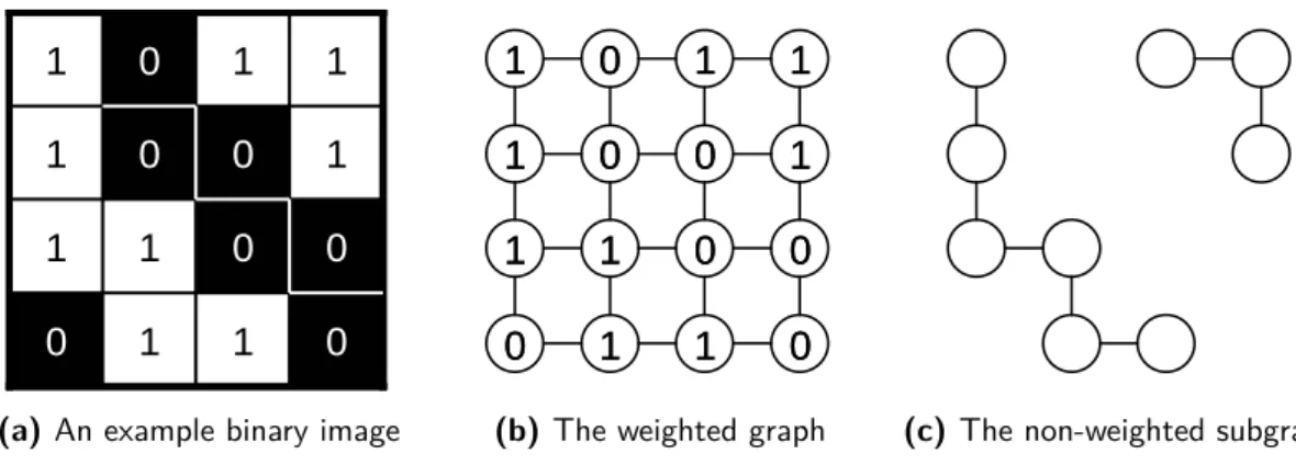
A binary image, which is a special case of the digital image with only two possible sample values, may be described in the following two ways, which are shown in Figure 2.3:
• as the weighted graph G = (V, E, f ) described above with the vertex weight function f : V → {0, 1}. Vertices with weight 0 are called background pixels and vertices with weight 1 are called foreground pixels.
• as a non-weighted subgraph GX= (X, EX) induced by the set of foreground pixels:
X = {v ∈ V : f (v) = 1}, EX = E ∩ (X × X). Note that information about the background regions is
dropped in this case.
2.1.2
Connected component tree (CCT)
A connected component C of the binary image is a maximal connected subset of its foreground pixels [Wilkinson 2008]. For example, the binary image shown inFigure 2.3contains two connected components.
The non-empty subset C ⊂ X is a connected component of graph GX = (X, EX) precisely if C is
connected in GX and there exists no vertex x ∈ X \ C such that C ∪ {x} is also connected in GX
0
1
1
0
0
0
1
1
1
0
0
1
1
1
0
1
0
1
1
0
0
0
1
1
1
0
0
1
1
1
0
1
(a) An example binary image
0
1
1
0
0
0
1
1
1
0
0
1
1
1
0
1
0
1
1
0
0
0
1
1
1
0
0
1
1
1
0
1
(b) The weighted graph (c) The non-weighted subgraph
Figure 2.3: Two possible descriptions of a binary image
The connected components of a grayscale image (also called peak components or domes [Wilkinson 2008]) are the connected components of all thresholdings of the image [Wilkinson 2008].
The non-empty subset C ⊂ V is a connected component of the image G = (V, E, f ) precisely if C is connected in G and there exists no vertex x ∈ V \ C such that f (x) ≥ min{f (v) : v ∈ C} and
C ∪ {x} is also connected in G.
The set of all connected components of the grayscale image is denoted by CC ⊂ 2V.
The value min(C) = min{f (v) : v ∈ C} is called the minimum or level [Salembier 1998] or altitude [Najman 2006] of component C.
An inclusion relation organizes all connected components of the grayscale image into a rooted tree structure called the connected component tree (CCT), where the parent of component C2 is the smallest component
C1 that is larger than C2 and contains C2. Figure 2.4shows an example.
The component C1 is the parent of C2 precisely if C2 ( C1 and there is no other component C3
such that C2( C3( C1. We write C1= P arent(C2). Parent of the root component is undefined.
We call the core C0of the component C the set of its pixels with level equal to the minimum of the component.
C0= {v ∈ C : f (v) = min(C)}.
It is obvious that the points of the component’s core belong to none of the component’s descendants and therefore each point of the image belongs to precisely one component core. The component is the union of its core and of the cores of all its descendants. All practical CCT representations for storage in computer memory exploit this property by storing only the cores of the components.
The leaves of the connected component tree described above contain local maxima of the image. The tree is therefore called a max-tree. By duality, if all comparisons concerning the weight function f are reversed and the minimum and maximum operators on f are swapped, a min-tree will be obtained whose leaves contain local minima. Unless stated otherwise, the following text concerns with the max-tree variant of the CCT, but the appropriate dual form of all statements applies to the min-tree as well.
1
1
0
0
5
5
4
4
2
2
2
2
5
5
3
3
0
0
(a) A grayscale image
(pixel values taken from [Ngan 2007])
f ≥ 0
f ≥ 1
f ≥ 2
f ≥ 3
f ≥ 4
f ≥ 5
(b) Thresholdings of the image at all possible
levels with connected components labeled
● ● ● ● ● ● ● ● ● ● ● ● ● ● ● ● ● ● ● ● ● ● ● ● ● ● ● ● ● ● ● ● ● ● ● ● ● ● ● ● ● ● ● ● ● ● ● ● ● ● ● ● ● ● ● ● ● ● ● ● ● ● ● ● ● ● ● ● ● ● ● ● ● ● ● ● ● ● ● ● ● ● ● ● ● ● ● ● ● ● ● ● ● ● ● ● ● ● ● ● ● ● ● ● ● ● ● ●
C
1C
2C
3C
5C
4C
6C
7 ● ● ● ● ● ● ● ● ● ● ● ● ● ● ● ● ● ●root
(c) The connected
com-ponent tree. Comcom-ponent core pixels are gray
Figure 2.4: A connected component tree example
2.2
CCT representations
The information contained in the CCT consists of two parts: • Parent/child relationships among the components of the CCT • The shape of each component, that is the set of pixels contained in it
Figure 2.5shows the classic and straightforward representation of the CCT. It is a tree, in which each node represents one connected component of the image, with parent/child relations among the nodes reflecting the parent/child relations among the components. The shapes of the components are represented by an injective relation between the tree nodes and the points of the image: Each tree node is in relation with the points of the corresponding component core. The inverse relation is called component mapping M : V → CC [Najman 2006]. This relation can be stored in two ways: Each tree node contains the list of the core’s pixels and/or each pixel holds a reference to the corresponding tree node.
There is also another CCT representation called point tree [Meijster PhD,Wilkinson 2008] which is inspired by the data structure used in the Tarjan’s union-find algorithm [Tarjan 1975]. It is shown in Figure 2.6b. As the name suggests, the pixels of the image themselves are organized into a tree, which is constructed in such a way that both the parent/child relationships among the components and the component shapes are retained:
● ● ● ● ● ● ● ● ● ● ● ● ● ● ● ● ● ● ● ● ● ● ● ● ● ● ● ● ● ● ● ● ● ● ● ● ● ● ● ● ● ● ● ● ● ● ● ● ● ● ● ● ● ● ● ● ● ● ● ● ● ● ● ● ● ● ● ● ● ● ● ● ● ● ● ● ● ● ● ● ● ● ● ● ● ● ● ● ● ● ● ● ● ● ● ● ● ● ● ● ● ● ● ● ● ● ● ●
C
1C
2C
3C
5C
4C
6C
7 ● ● ● ● ● ● ● ● ● ● ● ● ● ● ● ● ● ●root
(a) The CCTC
1C
2C
3C
4C
5C
6C
7root
(b) Its classic representation. Solid lines – the component mapping.
Dashed lines – the parent/child relationships among the components
Figure 2.5: The classic representation of the CCT
● ● ● ● ● ● ● ● ● ● ● ● ● ● ● ● ● ● ● ● ● ● ● ● ● ● ● ● ● ● ● ● ● ● ● ● ● ● ● ● ● ● ● ● ● ● ● ● ● ● ● ● ● ● ● ● ● ● ● ● ● ● ● ● ● ● ● ● ● ● ● ● ● ● ● ● ● ● ● ● ● ● ● ● ● ● ● ● ● ● ● ● ● ● ● ● ● ● ● ● ● ● ● ● ● ● ● ●
C
1C
2C
3C
5C
4C
6C
7 ● ● ● ● ● ● ● ● ● ● ● ● ● ● ● ● ● ●root
(a) The CCT 0 0 0 0 1 1 2 2 3 3 4 4 5 5 5 5 2 2root
C'
1C'
2C'
3C'
5C'
4C'
6C'
7(b) A general point tree
root
C'
1C'
2C'
3C'
5C'
4C'
6C'
7 0 0 0 0 1 1 3 3 4 4 5 5 5 5 2 2 2 2(c) The canonical point tree
Figure 2.6: The point tree. Each tree node in (b) and (c) shows the position of the pixel and its intensity value
in the image. For the canonical point tree, the rule to select the level roots was “select the rightmost pixel of the bottommost pixels”
• Points of one component core form a tree whose shape is irrelevant and whose root is called the component’s level root. The choice of the component’s level root is also irrelevant.
• The level root’s parent is an arbitrary point of the parent component’s core. The level root of the root component is the root of the point tree.
The point tree definition allows some freedom and therefore a given CCT may be represented correctly by different point trees. Working with trees will be usually faster, if the average depth of the nodes is small. It is therefore good if parents of the tree nodes are level roots. If this is fulfilled for all nodes (except for the root which has no parent), then we say that the point tree is perfectly compressed.
A perfectly compressed point tree, in which the choice of the component level roots has been fixed using some deterministic rule (for example, “select the point with the highest address”), is unique for a given CCT. Such point tree is called canonical [Berger 2007] and it is shown inFigure 2.6c.
Both the classic and the point tree CCT-representations use a rooted tree. The parent/child relationships in this tree have to be stored as references from each tree node to its parent node and/or to its child nodes. This suggests that there are two possible directions of these references:
• If parents point to their children, it will be possible to browse the entire tree from a single starting node, the root node. However, the number of children of a given node is not known a priori. Therefore, the references have to be stored in dynamic lists, which are complex and require a significant amount of memory.
• If children point to their parents, it will be possible to access ancestor nodes of a given node. Because every node except the root has exactly one parent, only one reference per node is stored which is very memory-efficient.
The third, most memory-demanding possibility is to store the references in both directions, which will allow browsing the entire tree from any starting node.
Any CCT representation described here may be converted to any other in linear time.
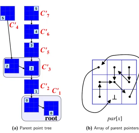
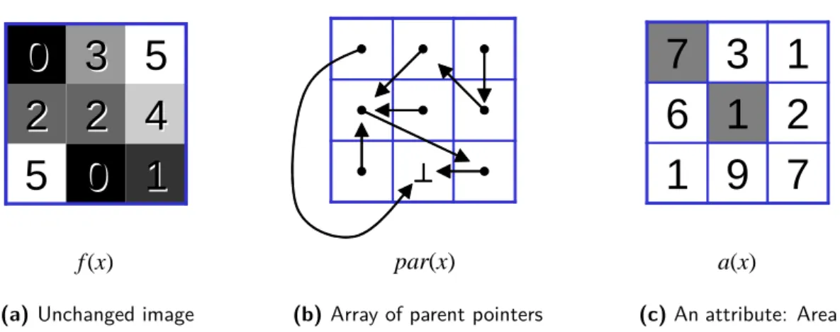
In this work, the CCT will be represented with the point tree with the references in the direction from children to their parents – a parent point tree that is used in many recent works [Meijster PhD,Berger 2007, Wilkinson 2008]. It is shown inFigure 2.7. It is the least memory demanding solution and it will allow an efficient implementation of tree merging, which will be necessary for parallelization of tree construction.
2.3
Attributes
The CCT on its own may be sufficient for some image transformations like watershed segmentation. Other operations on the image, especially filtering, require some aggregate knowledge about each component. This knowledge is expressed by component attributes. These are some numeric values characterizing each component.
Let us consider a connected component C ⊂ V of an image G = (V, E, f ). The following list mentions many simple attributes of the component C and gives a precise formal definition for majority of them. Beware however, that literature often presents identically named attribute definitions, which are not equivalent.
0 0 0 0 1 1 2 2 3 3 4 4 5 5 5 5 2 2
root
C'
1C'
2C'
3C'
5C'
4C'
6C'
7(a) Parent point tree
⊥
⊥⊥
⊥⊥
⊥⊥
⊥
par[x]
(b) Array of parent pointers
Figure 2.7: The parent point tree and its storage in the array of parent pointers
1
2
2
3
5
5
6
7
2
2
2
2
5
5
7
7
6
6
5
5
3
3
1
1
1
2
2
3
5
5
6
7
2
2
2
2
5
5
7
7
6
6
5
5
3
3
1
1
C
f
f
Figure 2.8: Illustration of the attribute Area on a 1D signal. a(C) = |C| = 4
• Area: The number of pixels of the component [Couprie 1997].
a(C) = |C|
This attribute is sometimes called “volume” in the context of 3D images [Wilkinson 2008], but it is different from the Volume definition used in this document.
1
2
2
3
5
5
6
7
2
2
2
2
5
5
7
7
6
6
5
5
3
3
1
1
1
2
2
3
5
5
6
7
2
2
2
2
5
5
7
7
6
6
5
5
3
3
1
1
C
f
f
(a) Minimum: min(C) = 5
1
2
2
3
5
5
6
7
2
2
2
2
5
5
7
7
6
6
5
5
3
3
1
1
1
2
2
3
5
5
6
7
2
2
2
2
5
5
7
7
6
6
5
5
3
3
1
1
C
f
f
(b) Maximum: max(C) = 71
2
2
3
5
5
6
7
2
2
2
2
5
5
7
7
6
6
5
5
3
3
1
1
1
2
2
3
5
5
6
7
2
2
2
2
5
5
7
7
6
6
5
5
3
3
1
1
C
f
f
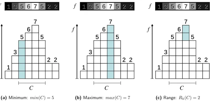
(c) Range: Rh(C) = 2Figure 2.9: Illustrations of attributes Minimum, Maximum, and Range
• Minimum: The minimum of the component’s pixel intensities. This attribute is also called Level h [Salembier 1998, Wilkinson 2008] or Altitude [Najman 2006] in the literature.
min(C) = min{f (v) : v ∈ C}
• Maximum [Deloison 2007]: The maximum of the component’s pixel intensities.
max(C) = max{f (v) : v ∈ C}
• Range: The difference between the maximum and minimum of the component. Sometimes it is also called Height [Couprie 1997]. This term will be avoided because it is sometimes used to refer to the Minimum attribute.
Rh(C) = max(C) − min(C)
• Parent’s minimum: The minimum of the parent component. The parent of the root component does not exist, so the value of this attribute has to be defined explicitly for the root component.
minp(C) = min(P arent(C)) if C is not the root component, minp(C) = min(C) − 1 if C is the root
component.
• Level difference: The difference of the minimum to the parent’s minimum. ∆min(C) = min(C) − minp(C)
• Core area: The number of pixels of the component’s core.
ac(C) = |C0| = |{v ∈ C : f (v) = min(C)}|
• Area difference for a given branch (inspired by [Sonka 2008]): The difference of the area of component C to the area of its son in the branch given by the component Cl⊆ C.
∆a(C, Cl) = |C \ [{Cs: Cs is a component of G ∧ P arent(Cs) = C ∧ Cl⊆ Cs}]| if Cl( C, ∆a(C, Cl) = |C| if Cl= C.
• Area difference to the parent (inspired by [Sonka 2008]): The difference of the area to the parent’s area. Again, special treatment of the root component is needed.
∆a(C) = a(P arent(C)) − a(C) if C is not the root component, ∆a(C) = 0 if C is the root component.
• Raw volume: The sum of the component’s pixel intensities.
Vr(C) =P
v∈Cf (v)
Note that the term “volume” is sometimes used to refer to the number of pixels of a 3D image component [Wilkinson 2008]. That attribute is called Area in this document.
• Volume above the component prism: The sum of differences of the component’s pixel intensities to the component minimum. It is the “volume” attribute from [Couprie 1997].
Vd(C) =Pv∈C(f (v) − min(C)) = Vr(C) − |C| · min(C)
• Proper volume: The sum of differences of the component’s pixel intensities to the parent’s minimum.
Vp(C) =Pv∈C(f (v) − minp(C)) = Vr(C) − |C| · minp(C)
• Perimeter [Deloison 2007]: The number of edges between the component and its complement.
P (C) = |E ∩ (C × (V \ C))|
• Roundness [Deloison 2007]: The ratio between the area and an appropriate power k ∈ R+ of the
perimeter. For a d-dimensional image, the choice k = d/(d − 1) makes the attribute invariant to scaling. This attribute may be used as an assessment of compactness of the component.
R(C) = |C|/(P (C))k
1
2
2
3
5
5
6
7
2
2
2
2
5
5
7
7
6
6
5
5
3
3
1
1
1
2
2
3
5
5
6
7
2
2
2
2
5
5
7
7
6
6
5
5
3
3
1
1
C
f
f
(a) Raw volume: Vr(C) = 23
1
2
2
3
5
5
6
7
2
2
2
2
5
5
7
7
6
6
5
5
3
3
1
1
1
2
2
3
5
5
6
7
2
2
2
2
5
5
7
7
6
6
5
5
3
3
1
1
C
f
f
(b) Volume above: Vd(C) = 31
2
2
3
5
5
6
7
2
2
2
2
5
5
7
7
6
6
5
5
3
3
1
1
1
2
2
3
5
5
6
7
2
2
2
2
5
5
7
7
6
6
5
5
3
3
1
1
C
f
f
(c) Proper volume: Vp(C) = 11• Moment of inertia [Wilkinson 2001]: Another measure component’s (non-)compactness. This one is based on pixel coordinates and it comes from physics.
If the pixels are treated as points with zero size, the following formula applies:
I(C) =P
v∈C||v − ¯v||
2, where the points v are treated as positional vectors, ¯v =P
v∈Cv/|C| is the
center of mass, and ||v|| is the norm of the vector v.
If the pixels are treated as squares or cubes with edge size equal to 1, then each pixel itself has some moment of inertia, which has to be added [Wilkinson 2001]:
I(C) = |C| · d/12 +P
v∈C||v − ¯v||
2, where d is the dimension of the image.
• Elongation [Wilkinson 2008]: A ratio between the Moment of inertia and Area, which is invariant to scaling.
φ1(C) = I(C)/|C|(d+2)/d, where d is the dimension of the image.
• Histogram entropy [Deloison 2007]: A statistic on the histogram of the component’s pixel intensities.
H(C) = −P
h∈Rp(h) log p(h), where p(h) = |{v ∈ C : f (v) = h}|/|C| is the percentage of the
component’s pixels having the intensity h, and 0 · log 0 = 0.
• Depth [Deloison 2007]: The distance between the component and the root in the component tree. In other words, it is the number of the component’s ancestors.
• Movement [Deloison 2007]: In a sequence of images, it is an assessment of how much the component has changed across different images of the sequence.
• Contrast: The standard deviation of the component’s pixel intensities. This attribute is called “SNR” in [Deloison 2007].
• Rate of change of the area with respect to the intensity (inspired by [Sonka 2008]): This attribute indicates how fast the component’s area changes with change of the threshold value. It is not defined for the root component.
a0(C) = ∆a(C)/∆min(C)
• Number of holes [Deloison 2007]: In the component’s complement V \C, it is the number of connected components with no pixels at the image border.
• Orientation (inspired by [Wilkinson 2008] and [Deloison 2007]): Another statistic based on pixel coordinates. This one indicates the angle or the directional vector of the direction, in which the component is elongated.
• Gradient energy [Deloison 2007]: The sum of the component’s pixel gradient magnitudes.
Many of these attributes are defined as an accumulation of some value over the pixels of the component or they can be derived from one or more such attributes. These attributes can be computed efficiently during the construction of the CCT without drastic increase of the execution time. Some other attributes may be computed efficiently too, but not before the complete tree has been constructed. There are also some attributes, which cannot be implemented efficiently, but it is often possible to find other, efficiently implementable attributes, which provide similar information.
An important property of each attribute is whether it is monotonic, that is whether the value of the attribute changes monotonically from a leaf to the root of the tree: An attribute A : 2V
→ R is increasing precisely if in every image G = (V, E, f ), for every two components C1 ⊆ C2 ⊆ V , the inequality A(C1) ≤ A(C2)
holds. An attribute fulfilling the reversed inequality is decreasing. An attribute is monotonic precisely if it is increasing or decreasing.
Here are some examples of increasing, decreasing, and non-monotonic attributes:
Increasing attributes: • Area • Maximum • Range • Volume • Moment of inertia • Gradient energy Decreasing attributes: • Minimum • Depth Non-monotonic attributes: • Perimeter • Roundness • Elongation • Histogram entropy • Number of holes
2.4
Examples of applications
2.4.1
Attribute filters
Image filtering is a typical example of a low-level operator, which aims at removing of noise from the image or at emphasizing of important features in it. The CCT-based filters work on the connected component tree of the image and delete unwanted nodes or branches from it. The resulting output image is reconstructed from the modified tree. A big advantage of these filters is that they do not introduce any new contours to the image. This is because each contour corresponds to a connected component, no new components are created in the process and the shapes of the components are preserved. The shapes in the original image are therefore either preserved or removed, but never modified.
The decision whether to keep or not each connected component is based on some criterion built upon the attributes whose form is usually A(C) ≥ λ, where A : 2V → R is some attribute and λ ∈ R is the criterion threshold. The direct decision rule is that the components, which fulfill the criterion, are kept, and those,
which do not, are deleted.
This direct decision rule works well for criterions built upon increasing attributes, so called increasing
criterions. In such criterions, if a given component is removed, then all of its descendants are removed too.
The image restitution from such tree is straightforward.
On the other hand, if the criterion is not increasing, then the direct decision rule may leave some components without their parents, in which case the nearest kept ancestor of the component will become its new parent. We say that the direct decision rule does not prune. A question how to reconstruct the image from such tree arises. Intuition says that some properties of the kept components should be conserved. These properties are described by attributes and a choice which attribute should conserve its values has to be made.
The classical choice is to conserve the Minimum attribute, in which case the intensity of each pixel in the image is lowered to the Minimum of the smallest kept component, which contains the pixel. The resulting filter is called a “direct filter”. It conserves well the absolute intensity levels in the image, but it produces steep jumps of intensity around the components, which are missing many ancestors in a row.
Conserving the Level difference attribute instead avoids this behavior. Such filter effectively subtracts the Level difference of each removed component from intensities of all image pixels belonging to the component. That is why the combination of the direct decision rule with the Level difference conservation is called a “subtractive filter”.
A few more attributes can be chosen for conservation, like the Raw volume for example.
To avoid leaving some components without their parents, other, pruning decision rules may be used. The “Min” decision rule keeps the component if it and all its ancestors fulfill the criterion. The “Max” decision rule keeps the component if it or any of its descendants fulfill the criterion. The “Optimal” decision rule [Salembier 1998] prunes the tree at the places, which lead to the lowest number of kept nodes not fulfilling the criterion and vice versa. This rule is also able to work with criterions formulated as a certainty that a given node should be preserved instead of a strict true/false assessment. The filter variants are shown in Figure 2.11.
Other modifications of the method are possible. One example is taking the residue of the filtration (the difference between the input and filtered images) as the result. Another example is keeping of n most important tree branches in which case the criterion threshold λ is set automatically.
An example attribute filtering result taken from [Wilkinson 2008] is shown inFigure 2.12.
f
(a) Input image (b) Direct filter (c) Subtractive filter
f
(d) Max filter (e) Optimal filter (f ) Min filter
Component which does NOT fulfill the criterion Component which DOES fulfill the criterion
Component fulfilling the criterion which was pruned away
(g) Legend
(a) Original image (b) Filtered image
Figure 2.12: An attribute filtering example. Maximum intensity projection of a 5123px CT angiogram, and the same volume filtered using the direct filter with the elongation criterion φ1(C) ≥ λ. Note the distinct suppression
of the background while retaining the vessel structure [Wilkinson 2008]
2.4.2
Segmentation 1: Detection of maximally stable extremal regions
Image segmentation is a high-level image processing operation, which aims at separating of objects from the background and/or of the individual objects from each other and/or at detecting of the boundaries between them. Section 5.3.11 of [Sonka 2008] mentions a segmentation method, whose description follows. It segments the image directly from the CCT, although the author does not refer to the CCT explicitly. This method detects significant bright (or dark, by duality) connected regions, which may be nested and may not cover the image entirely.
We have seen that we can construct the CCT from all thresholdings of the image. Let us imagine a movie consisting of such thresholded images, running from the highest to the lowest threshold. We would see the components emerge from the background, gradually grow, sometimes two or more components would touch and merge into one component, and the movie would end with a single component covering the entire image. In some ranges of threshold values, there may be components, whose areas respond very slowly to the threshold change, that means slower than in surrounding ranges. Such components are called maximally
stable extremal regions (MSERs). They are interesting, because each such component is significantly brighter
than its surroundings and therefore it is likely to correspond to some bright object in the registered scene. Figure 2.13 illustrates the principles of this method’s implementation, which is quite straightforward: Fig-ure 2.13ashows an input image,Figure 2.13bits level lines, andFigure 2.13cits connected component tree. Although Figures 2.13b and c show only 16 levels for simplicity, the actual CCT contains all 256 levels
(a) A grayscale image (b) Level lines
B
ra
n
c
h
1
B
ra
n
c
h
2
Root
(c) CCT(d) Maximally stable extremal regions
0 50 100 150 200 250 0 50 100 150 200 250 300 350 400 Level ∆a B ra n c h 1 B ra n c h 2
(e) Area difference function smoothed by a 6-tap weighted
moving average. Significant local minima are marked
Figure 2.13: A maximally stable extremal regions example
present in the input image. Now for each leaf Cl of the CCT, we compute the area difference attributes
∆a(C, Cl) for all components C in the corresponding CCT branch as a function of level h:
∆a(h, Cl) = ∆a([{C : C is a component of G ∧ Cl⊆ C ∧ min(C) = h}], Cl) if such component C
exists, ∆a(h, Cl) = 0 otherwise.
Then we perform some smoothing of this function and we seek for its significant local minima in each branch (Figure 2.13e). The components corresponding to such minima are the desired MSERs, i.e. the result of the segmentation (Figure 2.13d).