On Averaging the Best Samples in Evolutionary Computation
14
0
0
Texte intégral
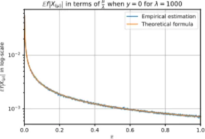
Figure

Documents relatifs