Alberta Lakes Thermodynamic Modelling.

(1)

Alberta Lakes Thermodynamic Modelling

by

Yves Gratton and Claude Bélanger

INRS-Eau, terre et environnement

Québec, Qc, Canada, G1K 9A9

Final report

(2)

2

ISBN : 978-2-89146-910-4 (version électronique)

Dépôt légal - Bibliothèque et Archives nationales du Québec, 2018 Dépôt légal - Bibliothèque et Archives Canada, 2018

Correct citation for this publication:

Gratton, Y. and C. Bélanger, 2018. Alberta Lakes Thermodynamic Modelling. Report No R1785, INRS-ETE, Québec (QC): 92 p.

(3)

3

List of Figures

Figure 1. Fish habitats. A lake can provide a) a complete habitat, b) a thermal and/or oxygen refuge, or c) no habitat at all. ... 9 Figure 2. Baptiste Lake. Source :

« http://albertalakes.ualberta.ca/?page=lake&region=1&lake=29 ». ... 13 Figure 3. Ethel Lake. Source : ... 14 Figure 4 Nakamun Lake. Source :

« http://albertalakes.ualberta.ca/?page=lake&region=1&lake=39 ». ... 15 Figure 5 Baptiste Lake, north basin. Temperature observations (blue dots) and modelled temperatures at selected depths (green lines) between May 2003 and February 2008. .... 18 Figure 6 Baptiste Lake, south basin. Temperature observations (blue dots) and modelled temperatures at selected depths (green lines) between May 2003 and February 2008. .... 18 Figure 7. Ethel Lake. Temperature observations (blue dots) and modelled temperatures at selected depths (green lines) between May 1980 and August 1984. ... 19 Figure 8. Nakamun Lake. Temperature observations (blue dots) and modelled

temperatures at selected depths (green lines) between May 2003 and February 2008. .... 19 Figure 9. Examples of deltas between 1981-2010 and 2071-2100: a) air temperature for February, b) wind speed for July, c) precipitations for March, d) global radiation for June, and e) cloud cover for May. ... 22 Figure 10. Average monthly deltas over Alberta for the periods 2041-2070 (magenta) and 2071-2100 (orange) for a) air temperature, b) wind speed, c) precipitations, d) global radiation and e) cloud cover. ... 23 Figure 11. Ethel Lake (1981-2010): fits versus data for days 244 and 245. ... 25 Figure 12. Baptiste Lake North (1981-2010): fits versus data for days 142, 147, 148, 229 and 251. ... 26 Figure 13. Data from the Split and Merge method fitted with third-order polynomials. This approach enables us to get rid of the spurious dip in the hypolimnion depths in august (month 08) and September (month 09). ... 27 Figure 14. Baptiste Lake, north basin. Contours of daily water temperature for 1981-2010 (top panel) and 2041-2070 (middle panel). The bottom panel is the difference between the two uppers panels (future - past). ... 29 Figure 15. Baptiste Lake, north basin. Contours of daily water temperature for 1981-2010 (top panel) and 2071-2100 (middle panel). The bottom panel is the difference between the two uppers panels (future - past). ... 29 Figure 16. Baptiste Lake, south basin. Contours of daily water temperatures for 1981-2010 (top panel) and 2041-2070 (middle panel). The bottom panel is the difference between the two uppers panels (future - past). ... 30 Figure 17. Baptiste Lake, south basin. Contours of daily water temperatures for 1981-2010 (top panel) and 2071-2100 (middle panel). The bottom panel is the difference between the two upper panels (future - past). ... 30 Figure 18. Ethel Lake. Contours of the daily water temperatures for 1981-2010 (top panel) and 2041-2070 (middle panel). The bottom panel is the difference between the two uppers panels (future - past). ... 31

(5)

5

Figure 19. Ethel Lake. Contours of the daily water temperatures for 1981-2010 (top panel) and 2071-2100 (middle panel). The bottom panel is the difference between the two uppers panels (future - past). ... 31 Figure 20. Nakamun Lake. Contours of the daily water temperatures for 1981-2010 (top panel) and 2041-2070 (middle panel). The bottom panel is the difference between the two uppers panels (future - past). ... 32 Figure 21. Nakamun Lake. Contours of the daily water temperatures for 1981-2010 (top panel) and 2071-2100 (middle panel). The bottom panel is the difference between the two uppers panels (future - past). ... 32 Figure 22. Example of indicator map: Average temperature over 0-5 m. Ethel Lake is moved at the center of the 385 grid points and the local NARR meteorological data is used to force the model. ... 33 Figure 23. Average surface (0-5 m) summer (JJA) temperature for BPTN: 1981-2010 (left), 2041-2070 (center) and 2071-2100 (right). ... 45 Figure 24. Increase in BPTN average surface temperature for 2041-2070 (left) and 2071-2100 (right). ... 46 Figure 25. Average surface (0-5 m) summer (JJA) temperature for BPTS: 1981-2010 (left), 2041-2070 (center) and 2071-2100 (right). ... 47 Figure 26. Increase in BPTN average surface temperature for 2041-2070 (left) and 2071-2100 (right). ... 48 Figure 27. Average surface (0-5 m) summer (JJA) temperature for ETL: 1981-2010 (left), 2041-2070 (center) and 2071-2100 (right). ... 49 Figure 28. Increase in ETL average surface temperature for 2041-2070 (left) and 2071-2100 (right). ... 50 Figure 29. Average surface (0-5 m) summer (JJA) temperature for NKM: 1981-2010 (left), 2041-2070 (center) and 2071-2100 (right). ... 51 Figure 30. Increase in NKM average surface temperature for 2041-2070 (left) and 2071-2100 (right). ... 52 Figure 31. Normalized heat content for BPTN (upper left), BPTS (upper right), ETL (lower left) and NKM (lower right). ... 54 Figure 32. Increase in maximum heat content between 1981-2010 and 2041-2070 for BPTN (upper left), BPTS (upper right), ETL (lower left) and NKM (lower right). ... 55 Figure 33. Increase in maximum heat content between 1981-2010 and 2071-2100 for BPTN (upper left), BPTS (upper right), ETL (lower left) and NKM (lower right). ... 56 Figure 34. Duration of the ice cover for BPTS: 1981-2010 (left), 2041-2070 (center) and 2071-2100 (right). ... 62 Figure 35. Decrease in duration of the ice cover (days) for BPTS: between 1981-2010 and 2041-2070 (left), and between 1981-2010 and 2071-2100 (right). ... 63 Figure 36. Duration of the ice cover for NKM: 1981-2010 (left), 2041-2070 (center) 2071-2100 (right). ... 64 Figure 37. Decrease in duration of the ice cover (days) for NKM: between 1981-2010 and 2041-2070 (left), and between 1981-2010 and 2071-2100 (right). ... 65 Figure 38. First day with ice cover for BPTS: 1981-2010 (left), 2041-2070 (center) and 2071-2100 (right). ... 66 Figure 39. Delay of the first day with ice cover (days) for BPTS: between 1981-2010 and 2041-2070 (left), and between 1981-2010 and 2071-2100 (right). ... 67

(6)

6

Figure 40. First day with ice cover for NKM: 1981-2010 (left), 2041-2070 (center) and 2071-2100 (right). ... 68 Figure 41. Delay of the first day with ice cover (days) for NKM: between 1981-2010 and 2041-2070 (left), and between 1981-2010 and 2071-2100 (right). ... 69 Figure 42. First day without ice cover for BPTS: 1981-2010 (left), 2041-2070 (center) 2071-2100 (right). ... 70 Figure 43. Advance of the first day without ice cover (days) for BPTS: between 1981-2010 and 2041-2070 (left), and between 1981-1981-2010 and 2071-2100 (right). ... 71 Figure 44. First day without ice cover for NKM: 1981-2010 (left), 2041-2070 (center) and 2071-2100 (right). ... 72 Figure 45. Advance of the first day without ice cover (days) for NKM: between 1981-2010 and 2041-2070 (left), and between 1981-1981-2010 and 2071-2100 (right). ... 73 Figure 46. Maximum ice thickness (cm) for BPTS: 1981-2010 (left), 2041-2070 (center) and 2071-2100 (right). ... 74 Figure 47. Decrease in maximum ice thickness (cm) for BPTS: between 1981-2010 and 2041-2070 (left), and between 1981-2010 and 2071-2100 (right). ... 75 Figure 48. Maximum ice thickness (cm) for NKM: 1981-2010 (left), 2041-2070 (center) and 2071-2100 (right). ... 76 Figure 49. Decrease in maximum ice thickness (cm) for NKM: between 1981-2010 and 2041-2070 (left), and between 1981-2010 and 2071-2100 (right). ... 77 Figure 50. Occurrence of the maximum ice thickness for BPTS: 1981-2010 (left), 2041-2070 (center) and 2071-2100 (right). ... 78 Figure 51. Advance of the maximum ice thickness for BPTS: between 1981-2010 and 2041-2070 (left), and between 1981-2010 and 2071-2100 (right). ... 79 Figure 52. Occurrence of the maximum ice thickness for NKM: 1981-2010 (left), 2041-2070 (center) and 2071-2100 (right). ... 80 Figure 53. Advance of the maximum ice thickness for NKM: between 1981-2010 and 2041-2070 (left), and between 1981-2010 and 2071-2100 (right). ... 81 Figure 54. Top of the metalimnion and hypolimnion for Baptiste-North, for 1981-2010. The red lines are obtained with the split and merge method while the black lines are three term polynomial fits. ... 85 Figure 55 Top of the metalimnion and hypolimnion for Baptiste-South, for 1981-2010. The red lines are obtained with the split and merge method while the black lines are three term polynomial fits. ... 85 Figure 56. Top of the metalimnion and hypolimnion for Ethel, for 1981-2010. The red lines are obtained with the split and merge method while the black lines are three term polynomial fits. ... 86 Figure 57. Top of the metalimnion and hypolimnion for Nakamun, for 1981-2010. The red lines are obtained with the split and merge method while the black lines are three term polynomial fits. ... 86 Figure 58. Top of the metalimnion and hypolimnion for Baptiste-North, for 2041-2070. The red lines are obtained with the split and merge method while the black lines are three term polynomial fits. ... 87 Figure 59. Top of the metalimnion and hypolimnion for Baptiste-South, for 2041-2070. The red lines are obtained with the split and merge method while the black lines are three term polynomial fits. ... Erreur ! Signet non défini.

(7)

7

Figure 60. Top of the metalimnion and hypolimnion for Ethel, for 2041-2070. The red lines are obtained with the split and merge method while the black lines are three term polynomial fits. ... 88 Figure 61. Top of the metalimnion and hypolimnion for Nakamun, for 2041-2070. The red lines are obtained with the split and merge method while the black lines are three term polynomial fits. ... 88 Figure 62. Top of the metalimnion and hypolimnion for Baptiste-North, for 2071-2100. The red lines are obtained with the split and merge method while the black lines are three term polynomial fits. ... 89 Figure 63. Top of the metalimnion and hypolimnion for Baptiste-South, for 2071-2100. The red lines are obtained with the split and merge method while the black lines are three term polynomial fits. ... Erreur ! Signet non défini. Figure 64. Top of the metalimnion and hypolimnion for Ethel, for 2071-2100. The red lines are obtained with the split and merge method while the black lines are three term polynomial fits. ... 90 Figure 65. Top of the metalimnion and hypolimnion for Baptiste-North, for 2071-2100. The red lines are obtained with the split and merge method while the black lines are three term polynomial fits. ... 90

(8)

8

List of Tables

Tableau 1. Some characteristics of the four lakes that were modelled. ... 12

Table 2. Mean, minimum and maximum average summer (JJA) temperature (°C) between 0-5 m and projected increases at the horizons 2041-2070 and 2071-2100 (scenario RCP 8.5). ... 44

Table 3. Mean, maximum and minimum normalized heat contents and projected increases in heat content (%) at the horizons 2041-2070 and 2071-2100 (scenario RCP 8.5). ... 53

Table 4. Mean, minimum and maximum duration of the ice cover and projected decreases at the horizons 2041-2070 and 2071-2100 (scenario RCP 8.5). ... 57

Table 5. Mean, earliest and latest occurrence of the first day with ice cover and projected ... 58

Table 6. Mean, earliest and latest occurrence of the first day without ice cover and projected advances at the horizons 2041-2070 and 2071-2100 (scenario RCP 8.5). ... 59

Table 7. Mean, minimum and maximum ice thickness (cm) and projected decreases at the horizons 2041-2070 and 2071-2100 (scenario RCP 8.5). ... 60

Table 8. Mean, earliest and latest occurrence of the maximum ice thickness and projected advances at the horizons 2041-2070 and 2071-2100 (scenario RCP 8.5). ... 61

Table 9. Dates of the thermocline. ... 82

Table 10. Maximum depth to the hypolimnion. ... 82

Table 11. Mean, minimum and maximum temperature of the epilimnion. ... 83

Table 12. Mean, minimum and maximum temperature of the metalimnion. ... 83

(9)

9

1. Introduction

Greenhouse gases accumulate in the atmosphere as a result of human activities. Taking into account likely future concentrations, global climate models predict an increase in air temperature of several degrees by the end of the twenty-first century and large changes in the regional distribution and intensity of precipitations (IPCC, 2013). These shifts in climate have already begun and are expected to modify the physical, chemical and biological attributes of lake water masses and affect their ability to maintain the present-day communities of aquatic plants, animals and microbes (Vincent, 2009). The possibility of significant change to many of the present lake ecosystems appears even more likely when considering that the majority of the world’s lakes are located between latitudes of about 47° and 73° N (Global Lakes and Wetland Database; Lehner and Döll, 2004), where warming is expected to be more pronounced (UNEP, 2012). Climate changes may affect directly the physical, chemical and biological characteristics of lakes, and also indirectly through modifications in the surrounding watershed. For dimictic boreal lakes, that is lakes that mix completely from surface to bottom twice a year, the most evident impacts include increased durations of ice-free conditions, increase in water column temperature and stronger stratification (vertical density structure) in summer. Larger future differences between air and surface water temperatures result in larger sensible heat transfer (conduction), and an earlier loss of snow and ice cover means a longer period of sensible heat transfer. Similarly, a shorter period of ice cover is expected to change the underwater irradiance regime and result in increased solar energy penetrating the water column. Both conductive and radiative effects lead to warmer surface waters in summer and stronger stratification which tends to lower downward transport of heat via turbulent mixing. One of the potential effects will be to modify fish habitats and their refuges. The shorter duration of the ice cover may also impact other aspects of the irradiance regime and lead to an increased availability of photosynthetically available radiation (PAR) for primary production as well as an increased exposure to ultraviolet radiation. All these physical changes (ice cover, temperature, stratification and mixing) may affect vertical gradients in lake properties and lead to significant effects on phytoplankton production and availability of food for higher trophic levels.

Climate changes are already affecting fish communities of northern lakes directly through the change in water

tempe-rature. Cold stenothermal fauna sensitive to even small changes in water temperature appears natu-rally more at risk. In addition to thermal stress, increased parasitism and competition could also

contribute to the decline of these endemic species (Vincent at al., 2011). The changes in temperature, light and nutrients availability may also have a qualitative effect on species

Figure 1. Fish habitats. A lake can provide a) a complete habitat, b) a thermal and/or oxygen refuge, or c) no habitat at all.

(10)

10

composition and diversity at the primary producer level (Peeters et al. 2007, Thackeray et al. 2008). An often-mentioned concern regarding this possibility is a shift toward dominance by species of cyanobacteria that form noxious bloom (Paerl & Huisman 2008). The overarching goal of the proposed project is to ensure the perenniality of the salmonid subsistence fisheries in northern lakes, such as Lake trout (Salvelinus namaycush) and Arctic char (Salvelinus alpinus), and the conservation of fish stocks for future generations. To attain that goal, we need a better understanding of the transformations of the lentic salmonid habitats, as defined by the spatial and the temporal variations of the extent of appropriate temperature-oxygen conditions for these fishes. All fish species have a preferred temperature range and a minimum oxygen level necessary for their survival. Lake trouts, for example, prefer water temperatures below 12° or 15 °C, depending on the authors, and oxygen levels (DO) above 4 or 6 mg l-1 (Plumb and Blanchfield, 2009). Some lakes can provide a suitable habitat all year round for a given species, while in other cases, only a small part of the lake is suitable during some period of the year, in summer for instance; these reduced habitats are called “refuges” (Fig. 1). In some cases, the preferred habitats can even disappear during part of the year. We propose to estimate possible changes in water temperature and ice cover duration for some lakes of Alberta for the horizons 2041-2070 and 2071-2100. A shift in the spatial distribution of many species can then be forecasted, some species being driven to extinction in some lakes while other species would be able to colonise the new warmer habitats. The practical applications of our results will be to improve tools for the managers of this important subsistence resource to help them optimize their fish population protection efforts and minimize the costs associated with securing the long-term perenniality of these species. The thermal habitat mapping that we will produce, combined with fish population data acquired by the managers will be used to map current and future fish productivity indexes and, in turn, help them decide on fish population management and habitat protection measures. Because of time constraints, this study simulates thermal habitats only, even if we made recent advances in oxic habitat simulations (Bélanger et al., 2017).

2. Objectives

The overarching goal of this study is to ensure the perenniality of subsistence and recreational fisheries in lakes and the conservation of fish stocks for future generations. The short-time goal is to estimate the potential shifts in lake water temperature of four lakes in the province of Alberta at the horizons of 2041-2070 and 2071-2100.

(11)

11

3. Method and Data

3.1 The lake model : MyLake

We used the one-dimensional model MyLake (Multi-year Lake model) to estimate past and future climatological annual cycles (in the sense of 30-year climatology) of water temperature and ice thickness in three Alberta lakes. Past and future annual cycles over the Alberta territory were also derived through virtually moving these lakes at 385 locations covering the entire province and running MyLake at each of these locations. MyLake was developed at the Norwegian Institute for Water Research (NIVA) (Saloranta and Andersen, 2007). In addition to simulating the evolution of temperature over the entire water column, MyLake also simulates the evolution of ice and snow covers. The model time step is 24 h and the required inputs are lake bathymetry (expressed as the area per meter of depth in our version), initial thermal conditions and time series of daily values for seven meteorological variables, namely air temperature, relative humidity, atmospheric pressure, wind speed, precipitations, radiation, and cloud cover. Time series of water temperature at different depths or, minimally, time series built from frequent vertical temperature profiles are needed to validate the simulations. Ice thickness data would be useful but are not essential.

3.2 The lakes

MyLake was prepared and calibrated for three Alberta lakes: Baptiste (BPT: 54.75°N, -113.55°W; 9.81 km2 and a maximum depth of 27.5 m), Ethel (ETL: 54.53°N and -110.35°W; 4.90 km2 _{and a maximum depth of 30 m), and Nakamun (NAK: 58.88°N,}

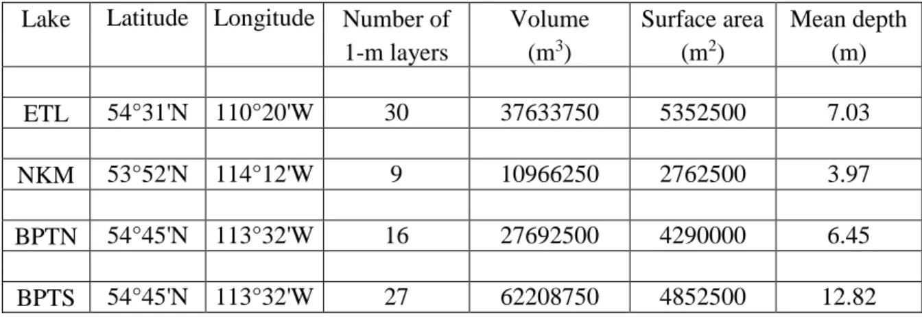
-114.20°W; 3.54 km2 and a maximum depth of 8 m). The northern (BPTN) and southern (BPTS) basins of Baptiste Lake were considered as two different lakes, giving a total of four lake models. These models were built using bathymetric data provided by Paul Drevnick (Alberta Environment and Parks). The four models specify the area at 1-m thick layers. There are 16 layers for BPTN, 27 layers for BPTS, 30 layers for ETL and 9 layers for NKM. From the volume and surface area, we estimated a mean depth of 6.45 for BPTN, 12.82 for BPTS (9.83 m for BPT when considering together both the northern and southern parts), 7.03 m for ETL and 3.97 for NKM. The mean depths given on the site albertalakes.ualberta.ca are slightly different, i.e. 8.6 m for BPT, 6.6 m for ETL and 4.5 m for NKM. The main characteristics of each of the four basins are presented in Table 1.

(12)

12

Tableau 1. Some characteristics of the four lakes that were modelled.

Lake Latitude Longitude Number of Volume Surface area Mean depth

1-m layers (m3) (m2) (m)

ETL 54°31'N 110°20'W 30 37633750 5352500 7.03

NKM 53°52'N 114°12'W 9 10966250 2762500 3.97

BPTN 54°45'N 113°32'W 16 27692500 4290000 6.45

(13)

13 3.2.1 Baptiste Lake

Baptiste Lake is moderate-sized lake with two basins joined by a long and shallow channel (Figure 2). The basins are of comparable sizes but the north basin is shallow (16 m) while the south basin is deep (28 m).

Figure 2. Baptiste Lake. Source :

(14)

14 3.2.2 Ethel Lake

Ethel Lake consists of four bays (Figure 3): a deep southwest bay with a maximum depth of 30 m, two northern bays with maximum depths of 8 m and 6 m, and a shallow southeast bay with a maximum depth of 3 m.

Figure 3.Ethel Lake. Source :

(15)

15 3.2.3 Nakamun Lake

Nakamun Lake is a medium-sized, fairly shallow lake that has a maximum length of 2.2 km and a maximum width of 0.8 km (Figure 4). The deepest area (8.0 m) is located in the centre of the basin

Figure 4 Nakamun Lake. Source :

(16)

16

3.3 The calibrations

The calibration consists in tuning diverse model parameters so the simulated temperature time series at all depths are as similar as possible to observed temperature time series. The temperature time series we used were built from temperature profiles provided by Paul Drevnick. All profiles (685 profiles) were inspected and edited to correct problems (e.g. depth inversions) when necessary. The profiles were interpolated in order to obtain temperature values at the center of the model layers (0.5 m, 1.5 m, 2.5 m, …) and time series at these depths were produced from the interpolated profiles. For calibration, the models were forced with meteorological observations at nearby weather stations, except for global radiation and cloud cover for which we used North American Regional Reanalysis (NARR) data at the closest grid point.

For both BPTN and BPTS, the calibration period we considered extends from 27 May 2003 to 26 Feb 2008 (five summers) and there were 28 temperature profiles available for that period. The prescribed initial conditions were derived from the profiles of 27 May 2003 (no ice cover). We used data from three weather stations for forcing: Dapp AGDM, Athabasca 2 and Athabasca 1 (about 60.8 km, 7.5 km and 24.1 km from BPT, respectively). Daily data of relative humidity and wind speed were derived from hourly data at Dapp AGDM. All gaps that were 9-hour long or shorter were filled using interpolation before deriving daily data. For gaps that were longer than 9 hours, daily values on those days were replaced daily NARR data at the grid point closest to BPT (about 15.2 km from the lake); that was done for 30 days out of 1737 days. For daily values of temperature and precipitations, we used daily data at station Athabasca 2. However, there were some important gaps in these data (160 days or 9.2 % of the period for temperature, 63 days or 3.6 % of the period for precipitations) and data from station Athabasca 1 were used on those days. There were only three days with no observation from either Athabasca 2 or Athabasca 1 and daily NARR data were used on those days. There were no atmospheric pressure data available for that period within 100 km from BPT. As for global radiation and cloud cover, we resorted to daily NARR data at the grid point closest to BPT.

For ETL, the calibration period we considered extends from 13 May 1980 to 28 Aug 1985 (five summers) and there were 62 temperature profiles available for that period. The prescribed initial conditions were derived from the profile of 13 May 1980 (no ice cover). We used data from Cold Lake station for forcing. Cold Lake station is about 13.6 km from ETL. Daily data of temperature, relative humidity, atmospheric pressure and wind speed were derived from hourly data after that some short gaps were filled using interpolation. Precipitations data were directly available as daily data. Daily NARR data at the grid point closest to ETL (about 8.8 km from the center of the lake) were used for global radiation and cloud cover.

For NKM, the calibration period we considered extends from 22 May 2003 to 9 Feb 2009 (six summers) and there were 32 temperature profiles available for that period. The prescribed initial conditions were derived from the profile of 22 May 2003 (no ice cover). We used data from two weather stations for forcing: Barrhead CS and Edmonton Stony

(17)

17

Plain CS (about 31.8 km 36.5 km from NKM, respectively). Daily data of temperature, relative humidity, atmospheric pressure and wind speed were derived from hourly data at station Barrhead CS. Most gaps were short ( 5 hours). These short gaps were filled using interpolation before deriving daily data. A 9.7-day gap in temperature and relative humidity data was filled using data from station Edmonton Stony Plain CS. Similarly, a long 36.2-day gap and a short 1.6-36.2-day gap in the wind speed time series were filled using data from the same station. For precipitations data, we used daily data at station Barrhead CS, except for nine days with no data; daily data from station Edmonton Stony Plain CS were used for those days. Daily NARR data at the grid point closest to NKM (about 3.5 km from the center of the lake) were used for global radiation and cloud cover.

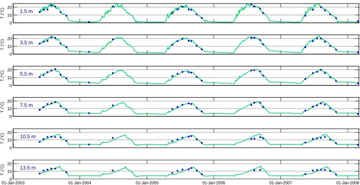
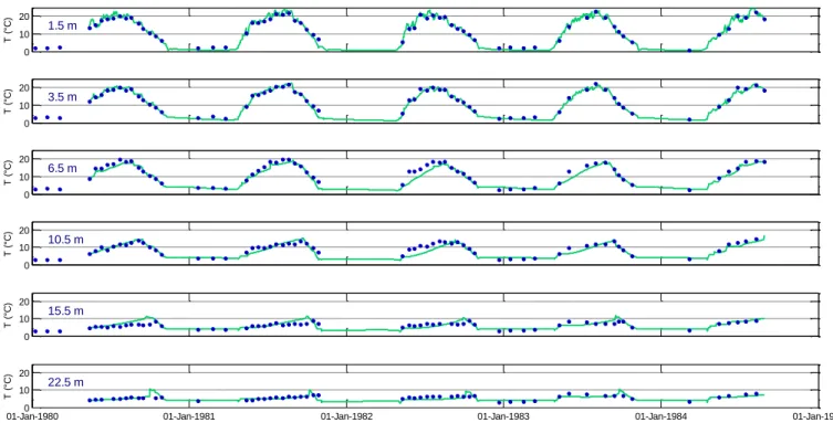
The figures 5 to 8 present a comparison of observed and simulated temperature time series at selected depths for BPTN, BPTS, ETL and NKM. The four models satisfactorily reproduce the observations over the entire water column.

(18)

18 0 10 20 T ( °C ) 1.5 m 0 10 20 T ( °C ) 3.5 m 0 10 20 T ( °C ) 5.5 m 0 10 20 T ( °C ) 7.5 m 0 10 20 T ( °C ) 10.5 m

01-Jan-20030 01-Jan-2004 01-Jan-2005 01-Jan-2006 01-Jan-2007 01-Jan-2008 10 20 T ( °C ) 13.5 m 0 10 20 T ( °C ) 1.5 m 0 10 20 T ( °C ) 3.5 m 0 10 20 T ( °C ) 6.5 m 0 10 20 T ( °C ) 10.5 m 0 10 20 T ( °C ) 16.5 m

01-Jan-20030 01-Jan-2004 01-Jan-2005 01-Jan-2006 01-Jan-2007 01-Jan-2008 10 20 T ( °C ) 24.5 m

Figure 5 Baptiste Lake, north basin. Temperature observations (blue dots) and modelled temperatures at selected depths (green lines) between May 2003 and February 2008.

Figure 6 Baptiste Lake, south basin. Temperature observations (blue dots) and modelled temperatures at selected depths (green lines) between May 2003 and February 2008.

(19)

19 0 10 20 T ( °C ) 0.5 m 0 10 20 T ( °C ) 1.5 m 0 10 20 T ( °C ) 2.5 m 0 10 20 T ( °C ) 3.5 m 0 10 20 T ( °C ) 5.5 m

01-Jan-20030 01-Jan-2004 01-Jan-2005 01-Jan-2006 01-Jan-2007 01-Jan-2008 01-Jan-2009 10 20 T ( °C ) 7.5 m 0 10 20 T ( °C ) 1.5 m 0 10 20 T ( °C ) 3.5 m 0 10 20 T ( °C ) 6.5 m 0 10 20 T ( °C ) 10.5 m 0 10 20 T ( °C ) 15.5 m

01-Jan-19800 01-Jan-1981 01-Jan-1982 01-Jan-1983 01-Jan-1984 01-Jan-1985 10 20 T ( °C ) 22.5 m

Figure 7. Ethel Lake. Temperature observations (blue dots) and modelled temperatures at selected depths (green lines) between May 1980 and August 1984.

Figure 8.Nakamun Lake. Temperature observations (blue dots) and modelled temperatures

(20)

20

3.4 Deriving the past and future annual cycles at the real locations

The annual cycles of temperature and ice thickness were produced using 30-year meteorological time series at the closest pixel (see Section 3.5). These time series were produced using reanalysis data from the North American Regional Reanalysis (NARR; Mesinger et al, 2006) for the past period (1981-2010) and deltas-modified reanalysis data for the future periods (2041-2070 and 2071-2100). A two-run strategy was used in order to provide realistic initial conditions. The first run of the past simulation was initialised using the average water temperature and ice and snow thickness of four January 1st of the calibration period (1981 to 1984 for ETL; 2004 to 2007 for NKM, BPTN and BPTS). The second run of the past simulation was initialised using the averages of temperature and ice and snow thickness of the last 15 January 1st of the first run’s output. The first run of the future simulations was initialised using the initial conditions used for the second run of the preceding period. As for the past simulation, the second run of the future simulations was initialised using the averages of temperature and ice and snow thickness of the last 15 January 1st of the first run’s output. The annual cycles were derived from the second run’s output averaging the 30 values (from 30 years) for each day of the year, i.e. average of 30 values on January 1st, average of 30 values on January 2nd, etc.

The annual cycles of past and future temperatures at the real lakes are presented in Section 4.

3.5 Deriving the past and future annual cycles across Alberta

Maps based on climatological water temperatures across Alberta and were produced from running MyLake at many contiguous pixels. The region between 49° and 60° N and -120 and -110° W has been divided into 440 pixels of 0.5° in latitude  0.5° in longitude (i.e. 22  20 pixels), with the center of the pixels at 49.25, 49.75, …, 59.75 °N and -119.75, -119.25, …, -110.25 °W. A mask prevents the model from being run at the pixels outside of the Alberta territory (440-55 = 385 pixels). The forcing time series for the reference period were built from averaging the NARR data inside each pixel. There were either one, two or three NARR grid point(s) in each pixel, corresponding to 30.9 %, 65.2 % and 3.9 % of the 440 pixels, respectively.

The annual cycles of past and future temperatures and ice and snow thickness at the 385 pixels were produced using 32-year meteorological time series at the each of the pixels. These time series were produced using NARR reanalysis data (for the past period, 1979-2010) and deltas-modified reanalysis data (for the future periods, 2039-2070 and 2069-2100). The model was run only once at each pixel, this involving that the specified initial conditions were identical for all pixels. In order to minimize the impact of the inexactitude in the initial conditions, the first two years of the simulated time series were not considered in the averaging process, leaving 30 years of simulated temperature and ice and snow thickness for averaging. That left-out initial two-year period can be viewed as a spinning time. For initial conditions, we used the initial conditions of the second run at the real lakes, both for past and future periods. As for the real lakes, the annual cycles were derived

(21)

21

averaging 30 values (from 30 years) for each day of the year, i.e. average of 30 values on January 1st, average of 30 values on January 2nd, etc.

The maps produced from running MyLake at 385 locations across the Alberta territory are presented in the Appendices II, III and IV.

3.6 The climate model and the deltas

Deltas are projected differences, for a given meteorological variable and for a given period of the year, between the reference period and a future period. Monthly deltas over the Alberta territory were derived from a climate simulation performed at Ouranos using the Canadian Regional Climate Model (simulation Ouranos_MRCC5_NAM-22_CCCma_CanESM2-run1). This simulation uses the greenhouse gas concentration scenario RCP 8.5. The Representative Concentration Pathways, or RCPs, are four greenhouse gas concentration trajectories adopted recently by the IPCC (IPCC 2014); the RCP 8.5 combines assumptions about high population and relatively slow income growth with modest rates of technological change and energy intensity improvements, leading in the long term to high energy demand and greenhouse gas emissions in absence of climate change policies. The future horizons we considered are 2041-2070 and 2071-2100.

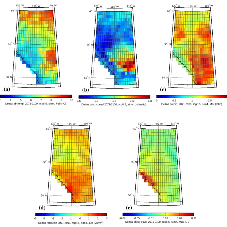
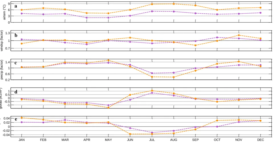
Monthly deltas at each of the 385 pixels were estimated for global radiation, cloud cover, air temperature, atmospheric pressure, wind speed and precipitations. (Relative humidity is assumed unchanged in the future and we expect this to have a negligible impact on the results.) The monthly deltas at a given pixel were derived using the values at the grid point of the climate model the closest to the center of the pixel. The average distance between the grid point and the center of the pixel is 9.33 km, with a minimum distance of 0.39 km and a maximum distance of 16.98 km. The figure 9 presents examples of delta spatial variations for five variables (air temperature, wind speed, precipitations, global radiations and cloud cover) for the horizon 2071-2100. In each case, we chose a month when the spatial variability is relative large. On the next figure (Fig. 5) we present an overview of the variability of the average monthly deltas for Alberta for both future horizons: 2041-2070 (magenta) and 2071-2100 (orange).

(22)

22

120 W 115 W 110 W

50 N 55 N

60 N

Deltas air temp. 2071-2100, rcp8.5, sim4, Feb (°C)

3 4 5 6 7 8 9 10

120 W 115 W 110 W

50 N 55 N

60 N

Deltas air temp. 2071-2100, rcp8.5, sim4, Feb (°C)

3 4 5 6 7 8 9 10

120 W 115 W 110 W

50 N 55 N

60 N

Deltas wind speed 2071-2100, rcp8.5, sim4, Jul (ratio)

0.6 0.9 1.2 1.5 1.8

120 W 115 W 110 W

50 N 55 N

60 N

Deltas precip. 2071-2100, rcp8.5, sim4, Mar (ratio)

0 0.5 1 1.5 2

120 W 115 W 110 W

50 N 55 N

60 N

Deltas radiation 2071-2100, rcp8.5, sim4, Jun (MJ/m2) -5 -4 -3 -2 -1 0 1 2 3

120 W 115 W 110 W

50 N 55 N

60 N

Deltas cloud cover 2071-2100, rcp8.5, sim4, May (0-1) -0.09 -0.05 -0.01 0.03 0.07 0.11

Figure 9.Examples of deltas between 1981-2010 and 2071-2100: a) air temperature for February, b) wind speed for July, c) precipitations for March, d) global radiation for June, and e) cloud cover for May.

(a) (b) (c)

(23)

23 0 3 6 9 a ir te m ( °C ) 0.7 1 1.3 w in d s p ( fa c to r) 0.2 0.6 1 1.4 p re c ip ( fa c to r) -1 -0.5 0 0.5 1 g lo ra d ( M J /m 2)

JAN FEB MAR APR MAY JUN JUL AUG SEP OCT NOV DEC

-0.04 -0.02 0 0.02 0.04 c lo c o v ( 0 -1 )

Figure 10.Average monthly deltas over Alberta for the periods 2041-2070 (magenta) and 2071-2100 (orange) for a) air temperature, b) wind speed, c) precipitations, d) global radiation and e) cloud cover.

b

c

d

e a

(24)

24

3.7 Identification of the three layers: epilimnion, metalimnion and hypolimnion

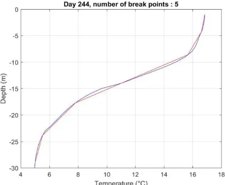
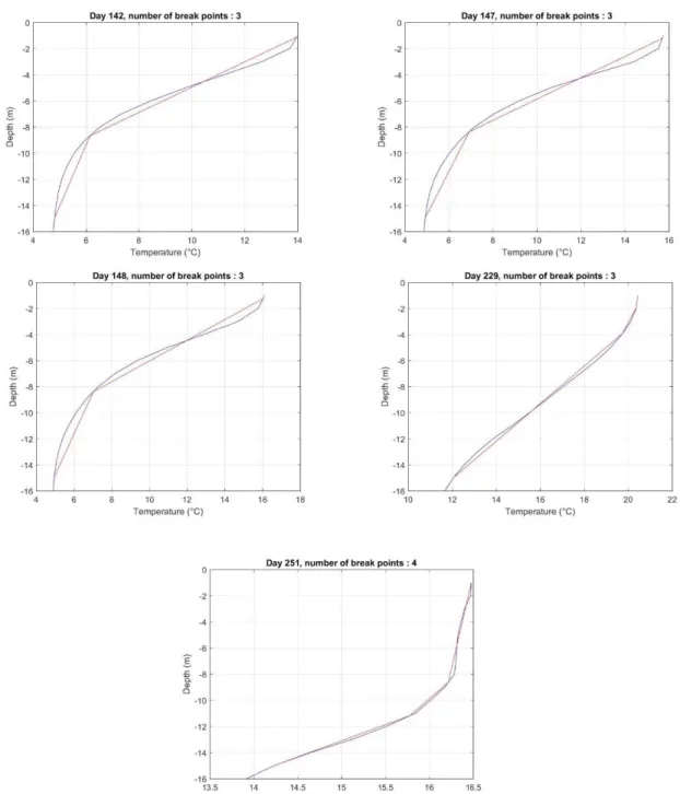
The identification of the three layers was performed in three steps. Firstly, we used a method called “Split and Merge” proposed by Thomson and Fine (2003). There are other methods but we already had the Matlab® code for this method. The Split and Merge method was developed, like most of the other methods, to pinpoint the base of the mixed layer in the ocean. It consists in fitting a set of linear segments to a density, temperature or salinity profiles. It then iterates to find the minimum number of segments that fits the observed profile within an error threshold. We chose a threshold of 0.04 to minimize the number of segments. The number of segment was 3 (most of the time), 4 (a few times) or 5 (very rarely). Secondly, we developed a script that uses the breakpoints (points where the slope of the linear segments changes) to identify the three layers. It was assumed that a water column with less than a 2° C differences between the first and last depth was a well mixed water column. We also postulated that a temperature difference of less than 2° C between the temperature at a break point location and the bottom would result in the setting the location of the top of the hypolimnion at that break point depth. Steps 1 and 2 are automatic processes: weird results are sometimes obtained. This is illustrated in Figures 11 and 12.

In figure 11, we observed a difference in the fit for successive days for Ethel Lake. The fit is a lot better (red line) on day 244 and the top of the hypolimnion is not at the same depth: 23 m for day 244 and 20 m for day 245. The epilimnion (mixed layer) is better characterized on day 244. The fits for five different days for Baptiste-North (1981-2010) are presented in figure 12. Days 142, 147 and 148 present examples where the epilimnion are very difficult to fit correctly. Days 229 and 251 present examples where the method yields hypolimnions only 1 m thick (the last m of the water column).

This led us to add a third step to our layer identification method. The output of the Split and Merge method was first smoothed with a three-point moving average (weights: 0.3, 0.4, 0.3). A third-degree polynomial was finally adjusted to the smoothed data to get rid of the spurious variations in the epilimnion and hypolimnion depths (see Figure 13). All the stratification indicators (Appendix V) were calculated using the polynomial fits.

(25)

25

Figure 11.Ethel Lake (1981-2010): fits (in red) versus data (in blue) for days 244 (top) and 245 (bottom).

(26)

26

Figure 12. Baptiste Lake North (1981-2010): fits (in red) versus data (in blue) for days 142 (top row, left), 147 (top row, right), 148 (middle row, left), 229 (middle row, right) and 251 (bottom row).

(27)

27

Figure 13. Data from the Split and Merge method (in red) fitted with third-order polynomials (in black). This approach enables us to get rid of the spurious dip in the hypolimnion depths in august (month 08) and September (month 09).

(28)

28

4. Simulated past and future annual cycles of temperature

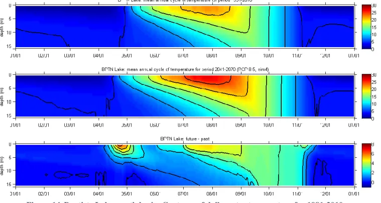
4.1 Baptiste Lake

Figures 11 to 14 present the contours of water temperature for Baptiste Lake North (Fig. 11 and 12) and South (Fig. 13 and 14) basins. There are three panels on each figure: the top panels are the temperature contours for the reference period 1981-2010 while the middle panels are the temperature contours for the period 2041-2070 (Figs. 13 and 15) or 2071-2100 (Figs. 14 and 16). The third panels present the difference between the future time period minus the reference time period, that is the differences between the first two panels. The equidistances for the contours of temperature and difference are 4 °C and 1 °C, respectively.

4.2 Ethel Lake

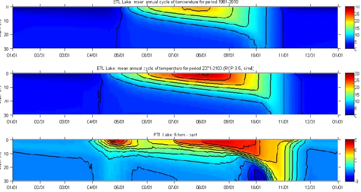
Figures 15 and 16 present the contours of water temperature for Ethel Lake. There are three panels on each figure: the top panels are the temperature contours for the reference period 1981-2010 while the middle panels are the temperature contours for the period 2041-2070 (Fig. 17) or 2071-2100 (Fig. 18). The third panels present the difference between the future time period minus the reference time period, that is the differences between the first two panels. The equidistances for the contours of temperature and difference are 4 °C and 1 °C, respectively.

4.3 Nakamum Lake

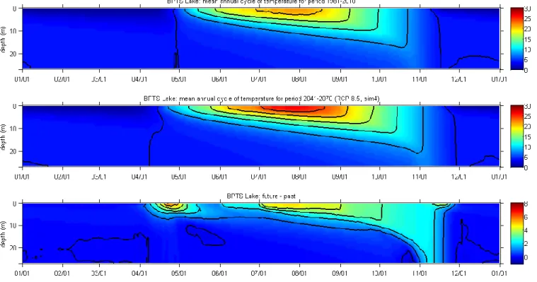
Figures 17 and 18 present the contours of water temperature for Nakamun Lake. There are three panels on each figure: the top panels are the temperature contours for the reference period 1981-2010 while the middle panels are the temperature contours for the period 2041-2070 (Fig. 17) or 2071-2100 (Fig. 18). The third panels present the difference between the future time period minus the reference time period, that is the differences between the first two panels. The equidistances for the contours of temperature and difference are 4 °C and 1 °C, respectively.

(29)

29

Figure 14.Baptiste Lake, north basin. Contours of daily water temperature for 1981-2010 (top panel) and 2041-2070 (middle panel). The bottom panel is the difference between the two uppers panels (future - past).

Figure 15.Baptiste Lake, north basin. Contours of daily water temperature for 1981-2010 (top panel) and 2071-2100 (middle panel). The bottom panel is the difference between the two uppers panels (future - past).

(30)

30

Figure 16. Baptiste Lake, south basin. Contours of daily water temperatures for 1981-2010 (top panel) and 2041-2070 (middle panel). The bottom panel is the difference between the two uppers panels (future - past).

Figure 17.Baptiste Lake, south basin. Contours of daily water temperatures for 1981-2010 (top panel) and 2071-2100 (middle panel). The bottom panel is the difference between the two upper panels (future - past).

(31)

31

Figure 18.Ethel Lake. Contours of the daily water temperatures for 1981-2010 (top panel) and 2041-2070 (middle panel). The bottom panel is the difference between the two uppers panels (future - past).

Figure 19.Ethel Lake. Contours of the daily water temperatures for 1981-2010 (top panel) and 2071-2100 (middle panel). The bottom panel is the difference between the two uppers panels (future - past).

(32)

32

Figure 20. Nakamun Lake. Contours of the daily water temperatures for 1981-2010 (top panel) and 2041-2070 (middle panel). The bottom panel is the difference between the two uppers panels (future - past).

Figure 21.Nakamun Lake. Contours of the daily water temperatures for 1981-2010 (top

panel) and 2071-2100 (middle panel). The bottom panel is the difference between the two uppers panels (future - past).

(33)

33

5. Alberta Habitat Indicator Maps

Appendix II presents the complete list of habitat indicators selected for this study. All maps are based on climatological water temperatures across Alberta and are produced from running the lake model at many contiguous pixels. Figure 21 presents one of the habitat indicators: a map of the volume-weighted average temperature for the reference period (1981-2010) for the depth range 0-5 m between 01 June and 31 August. In this case, the initial conditions on 01 January 1981 (temperature profile, ice thickness and snow thickness) were inferred from the simulated values on 01 January for the calibration period. The average water temperatures in summer appear to reflect latitude and terrain elevation. For example, the lower average temperature seen around 58.75° N and -115.5° W reflects the relatively high elevation of the Caribou Mountains (up to 1030 m), the highest mountains in northern Alberta. The remainder of the average temperature maps may be found in Appendix II.

In Appendices II, III, IV and V we present maps and tables of the following habitat indicators. All the data used to produce these maps and tables will be made available in ascii files.

Figure 22.Example of indicator map: Average temperature over 0-5 m. Ethel Lake is moved at the center of the 385 grid points and the local NARR meteorological data is used to force the model.

(34)

34

1. The summertime (June, July and August) average temperature for the 0-5 m layer and projected changes (based on climatological annual cycles)

The Appendix II presents maps of average water temperature for the upper part of the water column (0-5 m) between June 1st and August 31st. This is a volume-weighted average. The set of maps include reference past and both future horizons. The period of averaging was chosen so the simulated temperatures and derived rates of increase (°C decade-1) can be eventually compared to the observations-based rates of temperature increase provided in O’Reilly et al. (2015). This appendix also presents maps of projected change in average upper layer water temperature, expressed in °C. These maps provide information on the projected changes across the Alberta territory.

Mean, minimum and maximum values of average water temperature for the upper part of the water column (0-5 m) between June 1st and August 31st for all the pixels of the Alberta territory are presented in Table 2. The values for the projected increases are also presented. The largest mean of projected upper layer average summer temperature at the end of the century is 24.8 °C (for NKM, the lake with the smallest mean depth) while the largest mean of projected increase is 5.7 °C (also for NKM).

2. Heat content

- Maximum heat content (normalized) (based on climatological annual cycle for 1981-2010)

- Projected changes in maximum heat content (based on climatological annual cycles)

The Appendix III presents maps of normalized maximum heat content across the Alberta territory. They show the ratio between the maximum heat content at a given location and the absolute maximum heat content of all pixels. So there is only one pixel for which the normalized maximum heat content is one. These maps provides information on spatial variation of heat content, showing where are the regions with relatively cold and warm water temperatures at the core of summer. These maps were produced only for the reference period (1981-2010). This appendix also present maps of projected change in maximum heat content between reference past and future horizons (2041-2070 and 2071-2100). The increase is expressed as a percentage of the heat content for the reference period. These maps provide information on the relative magnitude of the expected changes and their spatial variations. For example, lakes in high elevation should undergo larger changes than lake at lower elevation. From a biological point of view, caution should be taken when considering these results since biological changes are sometimes linked to some tipping points, meaning that a given increase in heat content does not necessarily correspond to a proportionally equivalent biological change.

Mean and minimum values were computed for reference past and both future horizons (Table 3). The results suggest that spatial differences should tend to decrease in the future, the mean values over the Alberta territory slightly increasing with time while the minimum

(35)

35

values markedly increase. This appears to be mainly due to more pronounced projected changes at high elevation pixels.

3. Ice conditions

- Duration of the ice cover and projected changes (mean of 30 years) - First day with ice cover and projected changes (median of 30 years) - First day without ice cover and projected changes (median of 30 years) - Maximum of ice thickness and projected changes (based on climatological

annual cycles)

- Occurrence of the maximum of ice thickness and projected changes (based on climatological annual cycles)

The annexe IV presents five types of maps for ice conditions: 1) the duration of the period with ice cover, expressed in number of days, 2) the first day with ice cover, 3) the first days without ice cover, 4) the maximum of ice thickness, and 5) the occurrence of the maximum of ice thickness. The set of maps include reference past and both future horizons. As can be expected, the maps show that the duration of the ice cover increase with latitude and elevation. This appendix also presents maps of projected changes (i.e. decrease in duration of the period with ice cover, delay of ice-on, advance of ice-off, decrease in maximum ice thickness and advance of the maximum ice thickness). In general, the projected decreases in ice cover duration tend to be more pronounced in the south, even at low elevation pixels where the ice cover durations are relatively shorter.

Mean, minimum and maximum values across the Alberta territory for the five indicators are presented in Tables 4 to 8. The values for the projected changes are also presented. Based on the results for the four lakes, the projected average decrease in ice cover duration between 1981-2010 and 2041-2070 is 2.85 days decade-1, increasing to 4.83 days decade-1 over the next 30 years.

4. Appendix V. Water column stratification.

- Date of the appearance of the thermocline in the spring - Date of the disappearance of the thermocline in the fall - Length of the stratified period

- Maximum depth of the thermocline and its date of occurrence

- Maximum, minimum and mean temperature of the epilimnion, metalimnion and hypolimnion

(36)

36

6. Discussion

For each of the four Alberta lakes, we presented figures of past and future annual cycles of temperatures at all depths and difference between future and past. These figures show that the largest differences between future and past are related to an earlier warming and a later cooling in the future. The differences in spring are relatively large only near the surface. The differences in autumn reach the bottom due to the autumn mixing (exporting heat from near surface to depths) being delayed in the future. For the same reason, a negative difference can develop (future temperatures at depths lower than past temperatures), coinciding with the occurrence of the autumn mixing in the past. Some of these figures show a minor aberration: the temperature at depths becomes slightly below 4 °C in late autumn and then becomes slightly above 4 °C. Although small, this gain of heat is not realistic. This phenomenon appears to be an artifact of the averaging process favored by the very small vertical temperature gradient in the water column at that time of the year. This is not present in the figures for Ethel Lake.

Heat content gives an indication of temperature integrated over the entire water column. The maps of normalized maximum heat content (ratio of maximum heat content at a given location on maximum heat content of all locations) reflects the influence of latitude and terrain elevation on heat content. The locations with the largest values are in the southeast of the province and the locations with the smallest values are in the Rocky Mountains (roughly 60 % of the heat content in the southeast). The impact of terrain elevation is also visible in the north, the heat content ratio for the region of the Caribou Mountains (the highest mountains in northern Alberta, up to 1030 m) being smaller than at neighbouring pixels. The average projected increase in heat content is 17.6 % for the horizon 2041-2070 and 30.2 % for the horizon 2071-2100. The largest projected increases are in the high elevation regions and the smallest ones are in the southeast region. That means larger increases where it is relatively small and smaller increases where it is relatively large. That reflects in the increase of the minimum ratio from past to future (58.2 % for 1981-2010, 66.8 % for 2041-2070 and 71.7 % for 2071-2100), the difference between the warmest and coolest locations decreasing with time.

Maps of volume-weighted average water temperature between 0-5 m and between June 1st and August 31 resemble those of normalized heat content. That is because much of the heat content is from the upper layer (relatively warmer and more voluminous) and the maximum of heat content occurs during that period. The highest temperatures are in the southeast corner of the province and the lowest temperatures are at high elevation terrain. The mean value over Alberta is 18.4 °C and is projected to increase to 23.9 °C at the horizon 2071-2100. The maximum value over Alberta is 21.6 °C and is projected to increase to 26.7 °C at the horizon 2071-2100. The smallest projected increases are on the east side but not at the southernmost locations, rather between 51 and 53 °N. The largest projected increases are in the Rocky Mountains and on their lee side (although less pronounced in that area). The mean projected increase over Alberta is 3.3 °C between 1981-2010 and 2041-2070 and 5.5 °C between 2071-2100. From these values, we derive an increase of

(37)

37

0.55 °C decade-1 between 1981-2010 and 2041-2070, and of 0.73 °C decade-1 over the next 30 years. These are large values by comparison with the global mean observed increase in surface temperature for the same summer period (June-July-August) reported by O’Reilly et al. (2015), i.e. 0.34 °C decade-1 between 1985 and 2009. This gives an indication that the rate of change could more than double over 70 years (roughly 1997-2087).

Spatial variations of ice cover and projected changes were considered via five indicators: duration of the ice cover, occurrence of the first day with ice cover, occurrence of the first day without ice cover, maximum ice thickness and occurrence of the maximum ice thickness. The general pattern for the number of days with ice cover is to increase with latitude and terrain elevation. Between 53 and 56 °N, there is a tendency for the duration of the ice cover to be shorter on the west side of the province than on the east side. The mean duration of simulated ice cover across Alberta is 168.5 days for 1981-2010, and the projected decreases are 26.1 days at the horizon 2041-2070 and 45.9 days at the horizon 2071-2100 (corresponding to -4.4 days decade-1 between 1981-2010 and 2041-2070, accelerating to -6.6 days decade-1 over the next 30 years). Roughly, the delay of the ice-on accounts for 40 % of the projected decreases in duratiice-on and the advance of the ice-off accounts for 60 % (56.8 % between 2010 and 2041-2070 and 60.3 % between 1981-2010 and 2071-2100). (Note that the duration of ice cover was computed using the mean of 30 years while the occurrence of ice-on and ice-off were computed using the median of 30 years, hence resulting in the sum of the changes in ice-on and ice-off being slightly different, i.e. 0.4 days shorter for 2041-2070 and 0.7 days longer for 2071-2100). The maps of maximum ice thickness also show an increase with latitude and terrain elevation, and a tendency for increase from west to east below 56 °N. The projected decrease in maximum ice thickness is pronounced in the Rocky Mountains but contrastingly relatively small in the Caribou Mountains. The decreases are also relatively large for two sub regions, near the eastern border between 53 and 55 °N and north of 58 °N. The mean maximum of simulated ice thickness across Alberta is 53.4 cm for 1981-2010 and the projected decreases are 11.8 cm for the horizon 2041-2070 and 17.4 cm for the horizon 2071-2100 (corresponding to 2.0 cm decade1 between 19812010 and 20412070, accelerating to -5.8 cm decade-1 over the next 30 years). The average occurrence of the maximum ice thickness is March 22 for 1981-2010. The projected advances are 18.4 and 31.3 days, corresponding to the maximum thickness occurring on March 4 at the horizon 2041-2070 and February 19 at the horizon 2071-2100.

An unexpected finding is that ice cover may not form in the future for certain years at southern locations. That occurred only for the horizon 2071-2100 at six locations between 49.25 and 50.75 °N. (Because of these few cases, it was impossible to use the mean of thirty years to compute the climatological occurrence of ice-on and ice-off and so we resorted to using the median.) The results indicate that the complete absence of ice cover should be rare, i.e. one out of thirty years in five of the six cases, and two years for the other case. We recall however that the delta method implies that climate changes will not affect the inter-annual variability of the meteorological variables, which may seem unlikely. Consequently, the projected frequency of years without ice cover should be considered with caution.

(38)

38

It can be expected that a lake with larger mean depth accumulates more heat (per unit of surface) than a lake with a smaller mean depth. That is because the heat in the surface layer is diluted in a more voluminous sub-layer for the deeper lake, resulting in a lower surface temperature, resulting in turn in a larger transfer of heat in time of heat gain. As more heat is accumulated in summer in a deeper lake, and since the heat loss begins earlier in a shallower lake due to higher surface temperature, the temperature in autumn is higher for some time in a deeper lake. Some of the results match this behaviour. The average upper layer summer temperature is higher for the shallowest lake (NKM, mean depth of 4.0 m) than for the deepest lake (BPT-S, mean depth of 12.8 m). The average difference across Alberta is 1.27 °C for 1981-2010, increasing to 1.63 °C for 2041-2070 and 1.73 °C for 2071-2100. The higher temperatures in autumn lead to a later ice formation. The average ice formation occurs 6.9 days later at BPT-S than at NKM for 1981-2010, increasing to 7.1 days for 2041-2070 and 7.9 days for 2071-2100. The end of the ice cover ice tends to occur a little earlier for a deeper lake but the difference is much less important (in average, 1.0 day earlier for BPT-S than for NKM for 1981-2010). Consequently, the difference in duration of the ice covers between a relatively deep lake and a shallower lake appears much more related to the difference in the occurrence of ice-on than to the difference in the occurrence of ice-off. The ice formation beginning later in a deeper lake, we can expect that it leads to a slightly smaller maximum ice thickness. Accordingly, the difference in average maximum ice thickness between NKM and BPT-S is 3.7 cm for 1981-2010. It is increasing to 4.0 days for 2041-2070 but decreasing to 3.1 cm for 2071-2100. The reason for a smaller difference in maximum ice thickness for the horizon 2071-2100 is not clear; it results from a more slightly larger decrease between 2041-2070 and 2071-2100 for NKM than for BPT-S.

(39)

39

7. Summary and Conclusion

The evolution of water temperature and ice cover in three lakes of the Alberta territory was simulated with the help of a 1-D lake model (MyLake) forced by daily meteorological data. The considered lakes are Baptiste Lake (BPT), Ethel Lake (ETL) and Nakamun Lake (NKM). For Baptiste Lake, the northern and southern basins were modelled separately, giving a total of four modelled lakes. These lakes have different surface areas and bathymetric characteristics (see Table 1) susceptible to modulate the magnitude and timing of the evolutions of temperature and ice cover. Each of the four models was calibrated separately using meteorological observations at nearby weather stations and multi-year time series of water temperature. Past (1981-2010) annual cycles of climatological water temperature and ice cover were derived forcing the models with 30-year meteorological time series obtained from reanalysis data. Future (2041-2070 and 2071-2100) annual cycles were similarly derived, the future 30-year time series being obtained through modifying the past time series accordingly to the monthly average differences between future and past conditions (deltas) estimated with the Canadian Regional Climate model (CRCM5). Future annual cycles were derived for a single greenhouse gas concentration scenario, i.e. RCP 8.5, corresponding to the situation where the humanity would do little to fight climate change, leading in the long term to high energy demand and greenhouse gas emissions. In that context, the projected future conditions that are presented may be seen as being at the extremity of the range of the possible conditions in near futures. The past and future annual cycles were first derived at the real location of each lake. Then, similarly, past and future annual cycles were derived at 385 locations across the Alberta territory (running the model at each location) and 2-D maps were produced. This method involves that the lake environment does not change when virtually placed at another location. For example, a lake with forested shores (having an impact on wind speed and mixing) stays a lake with forested shores. Diverse maps of past and future conditions and projected changes were produced for each of the four lakes.

The work that was realised can be complemented in several ways.

- It would be relevant to state the number and percentage of Albertan lakes with size and bathymetric characteristics nearly similar to those of the four lakes that were considered, and where they are located.

- The smallest lake that was considered (NKM) is not very small (surface area of 2.76 km2 and mean depth of 4.0 m); it could be of interest to add a fifth smaller lake if such lakes are frequent in Alberta.

- The derivation of the annual cycles requires long forcing time series and relies on using reanalysis data. We used the North-American Region Regional (NARR) data. It would be of interest to verify if other available reanalysis data (e.g. CFSR) perform better (are closer to observations) across the Alberta territory.

- We considered only one greenhouse gas concentration scenario, i.e. RCP 8.5. Although it is reasonable to use a worse-case scenario in a context where trying to shed light on possible problematic conditions, it would be of interest to compare the projected changes for RCP 8.5 with projected changes for others scenarios. The monthly deltas for

(40)

40

Alberta are readily available for the scenario RCP 4.5, but from another model and with a different resolution.

- We used only one of two CRCM5 simulations run at Ouranos with the scenario RCP 8.5. It would be of interest to compare the monthly deltas produced from these two simulations to see how close/different they are. In case they are somewhat different, a possibility for future works would be to consider average deltas derived from both simulations.

- Much of the presented results is about ice cover and projected changes. It would be of interest to verify how well the model MyLake reproduces the evolution of the ice cover at each of the four lakes. Due to lack of readily available data, this aspect has not been considered at the calibration step.

- Maps of other indicators could be produced from the derived climatological annual cycles. These indicators would be chosen to answer specific questions. For example, such maps could answer questions on evolution of productivity and loss of habitat for given fish species (e.g. number of m3-degrees-days when the temperature is between specified lower and a upper limits, and minimum volume with temperature below a specified upper limit).

(41)

41

References

Bélanger, C., R.-M. Couture, T. Logan, Y. Gratton, A. St-Hilaire, I. Laurion, M. Rautio and P. del Giorgio (2017a). Northern salmonid habitat in the future: impacts of climate change on the spatial variability of their lentic habitat between 50°N and 75°N. Rapport submitted to Ouranos, August, 2017.

Bélanger, C., R.-M. Couture, Y. Gratton, I. Laurion, T. Logan, M. Rautio and A. St-Hilaire (2017b). Impacts of climate changes on dissolved oxygen concentrations in Québec Province lakes. Report No R1752 (http://espace.inrs.ca/6527/), INRS-ETE, Québec (QC): viii + 48 p.

Bélanger, C., D. Huard, Y. Gratton, D.I. Jeong, A. St-Hilaire, J.-C. Auclair, and I. Laurion (2013). Impacts des changements climatiques sur l’habitat des salmonidés dans les lacs nordiques du Québec, Rapport INRS – Eau, Terre, Environnement pour Ouranos, http://espace.inrs.ca/2404/, 167 p.

IPCC, 2014. Climate Change 2014: Synthesis Report. Contribution of Working Groups I, II and III to the Fifth Assessment Report of the Intergovernmental Panel on Climate Change [Core Writing Team, R.K. Pachauri and L.A. Meyer (eds.)]. IPCC, Geneva, Switzerland, 151 pp.

IPCC, 2013. Summary for policymakers. In Climate change 2013: The physical science basis. Contribution of Working Group 1 to the fifth Assessment Report of the

Intergovernmental Panel on Climate Change [Stocker, T.F., D. Qin, G.-K. Plattner, M. Tignor, S.K. Allen, J. Boschung, A. Nauels, Y. Xia, Bex , V. and P.M. Midgley (eds.)]. Cambridge University Press, Cambridge, United Kingdom and New York, NY, USA. Lehner, B. and P. Döll (2004). Development and validation of a global database of lakes, reservoirs and wetlands. J. Hydrol., 296: 1-22.

Mesinger F., G. DiMego, E. Kalnay, K. Mitchell, P.C. Shafran, W. Ebisuzaki, D. Jović, J. Woollen J, E. Rogers, E.H. Berbery, M.B. Ek, Y. Fan, R. Grumbine, W. Higgins, H. Li, Y. Lin, G. Manikin, D. Parrish, W. Shi, 2006. North American Regional Reanalysis. B. Am. Meteorol. Soc., DOI:10.1175/BAMS-87-3-343.

O’Reilly, C. M., et al. (2015). Rapid and highly variable warming of lake surface waters around the globe. Geophys. Res. Lett., 42, doi:10.1002/2015GL066235.

Paerl, H.W., and J. Huisman (2008). Blooms like it hot. Sciences, 320, 57-58.

Peeters, F., D. Straile, A. Lorke, and D.M. Livingstone (2007). Earlier onset of the spring phytoplankton bloom in lakes of the temperate zone in a warmer climate. Global Change Biology, 13, 1898-1909.

(42)

42

Plumb, J.M. and P.J. Blanchfield (2009). Performance of temperature and dissolved oxygen criteria to predict habitat use by lake trout (Salvelinus namaycush). Can. J. Fish. Aquat. Sci., 66: 2011-2023.

Saloranta, T.M. and T. Andersen (2007). MyLake – a multi-year lake simulation model suitable for uncertainty and sensitivity analysis simulations. Ecol. Model., 207, 45-60. Thackeray, S.J., I.D. Jones, and S.C. Maberly (2008). Long-term change in the phenology of spring phytoplankton: species-specific responses to nutrient enrichment and climatic change. Journal of Ecology, 96, 523–535.

United Nations Environmental Program (UNEP), 2012. Keeping track of our changing environment, 111 p.

Vincent, W. F. (2009). Effects of climate changes on lakes. in Encyclopedia of Inland

Waters (ed. G.E. Likens), Elsevier, Oxford, vol. 3, pp. 55–60.

Vincent, W.F., T.V. Callaghan, D. Dahl-Jensen, M. Johansson, K.M. Kovacs, C. Michel, T. Prowse, J.D. Reist, and M. Sharp (2011). Ecological implications of changes in the Arctic cryosphere. Ambio, 40: 87-99.

(43)

43

Appendix I :

MyLake Possible Input and Initial Variables

Daily inputs Initial profiles

year Z (m)

month Az (m2₎

day Tz (°C)

global_rad (MJ m-2₎ _{Cz (passive tracer)}

cloud_cov (-) Sz (kg m-3₎

air_temp (°C) TPz (mg m-3₎

rel_hum (%) DOPz (mg m-3₎

air_pres (hPa) Chlaz (mg m-3₎

wind_sp (m s-1₎ _{DOCz (mg m}-3₎

precip (mm day-1₎ _{TPz_sed (mg m}-3₎

inflow (m3_day-1₎ _{Chlaz_sed (mg m}-3₎

inflow_T (°C) Fvol_IM (m3_/m3_{, dry w.)}

inflow_C (passive tracer) Hice (m)

inflow_S (sediment tracer; kg m-3₎ _{Hsnow (m)}

inflow_TP (mg m-3₎ _{O2z (mg m}-3₎ inflow_DOP (mg m-3₎ inflow_chla (mg m-3₎ Inflow DOC (mg m-3₎ Inflow DIC (mg m-3₎ Inflow O (mg m-3₎ Inflow NO3 (mg m-3₎ Inflow NH4 (mg m-3₎ Inflow SO4 (mg m-3₎ Inflow Fe2 (mg m-3₎ Inflow Ca2 (mg m-3₎ Inflow pH Inflow CH4 (mg m-3₎ Inflow Fe3 (mg m-3₎ Inflow Al3 (mg m-3₎ Inflow SiO4 (mg m-3₎ Inflow SiO2 (mg m-3₎ Inflow diatom (-)

See Saloranta and Anderson (2005) and Couture et al. (2015) for more details.

Couture, R.-M., H.A. de Wit, K. Tominaga, P. Kiuru, and I. Markelov, 2015. Oxygen dynamics in a boreal lake responds to long-term changes in climate, ice

phenology and DOC inputs. J. Geophys. Res. Biogeosci., 120, 2441-2456, doi :10.1002/2015JG003065.

Saloranta, T.M. and T. Andersen, 2005. MyLake (v.1.2): Technical model documentation and user’s guide for version 1.2. NIVA, Oslo, Unpublished report, 32 p.

(44)

44

Appendix II : Volume-weighted Averaged 0-5 m Temperature

Table 2. Mean, minimum and maximum average summer (JJA) temperature (°C) between 0-5 m and projected increases at the horizons 2041-2070 and 2071-2100 (scenario RCP 8.5).

Mean, minimum and maximum of average temperature between 0-5 m for period JJA for Alberta (385 pixels)

Lakes ETL NKM BPTN BPTS 1981-2010, mean 18.42 19.10 18.35 17.83 2041-2070, mean 21.70 22.55 21.65 20.92 2071-2100, mean 23.91 24.79 23.87 23.06 1981-2010, minimum 9.66 10.42 9.43 9.32 2041-2070, minimum 14.62 15.43 14.48 14.11 2071-2100, minimum 17.53 18.19 17.58 16.85 1981-2010, maximum 21.57 22.20 21.55 20.90 2041-2070, maximum 24.91 25.73 24.91 24.05 2071-2100, maximum 26.68 27.62 26.70 25.77

Mean, minimum and maximum increase in average temperature between 0-5 m for period JJA for Alberta (385 pixels)

ETL NKM BPTN BPTS from 1981-2010 to 2041-2070, mean 3.28 3.46 3.29 3.10 from 1981-2010 to 2071-2100, mean 5.49 5.69 5.52 5.23 from 1981-2010 to 2041-2070, minimum 2.26 2.26 2.31 2.28 from 1981-2010 to 2071-2100, minimum 4.50 4.54 4.58 4.49 from 1981-2010 to 2041-2070, maximum 5.01 5.02 5.09 4.82 from 1981-2010 to 2071-2100, maximum 8.00 7.86 8.19 7.57

(45)

45

(46)

46

(47)

47