PLANIFICATION D'ACTIONS CONCURRENTES SOUS
CONTRAINTES ET INCERTITUDE
par
Eric Beaudry
These presentee au Departement d'informatique
en vue de I'obtention du grade de philosophiae doctor (Ph.D.)
FACULTE DES SCIENCES
UNIVERSITE DE SHERBROOKE
1*1
Published Heritage Branch 395 Wellington Street Ottawa ON K1A 0N4 Canada Direction du Patrimoine de I'edition 395, rue Wellington OttawaONK1A0N4 CanadaYour file Votre reference ISBN: 978-0-494-75069-8 Our file Notre reference ISBN: 978-0-494-75069-8
NOTICE: AVIS:
The author has granted a
non-exclusive license allowing Library and Archives Canada to reproduce, publish, archive, preserve, conserve, communicate to the public by
telecommunication or on the Internet, loan, distribute and sell theses
worldwide, for commercial or non-commercial purposes, in microform, paper, electronic and/or any other formats.
L'auteur a accorde une licence non exclusive permettant a la Bibliotheque et Archives Canada de reproduire, publier, archiver, sauvegarder, conserver, transmettre au public par telecommunication ou par I'lnternet, preter, distribuer et vendre des theses partout dans le monde, a des fins commerciales ou autres, sur support microforme, papier, electronique et/ou autres formats.
The author retains copyright ownership and moral rights in this thesis. Neither the thesis nor substantial extracts from it may be printed or otherwise reproduced without the author's permission.
L'auteur conserve la propriete du droit d'auteur et des droits moraux qui protege cette these. Ni la these ni des extra its substantiels de celle-ci ne doivent etre imprimes ou autrement
reproduits sans son autorisation.
In compliance with the Canadian Privacy Act some supporting forms may have been removed from this thesis.
Conformement a la loi canadienne sur la protection de la vie privee, quelques
formulaires secondaires ont ete enleves de cette these.
While these forms may be included in the document page count, their removal does not represent any loss of content from the thesis.
Bien que ces formulaires aient inclus dans la pagination, il n'y aura aucun contenu manquant.
1*1
Le 31 mars 2011
lejury a accepte la these de Monsieur Eric Beaudry dans sa version finale.
Membres du jury
Professeur Froduald Kabanza Directeur de recherche Departement d'informatique
Professeur Francois Michaud Codirecteur de recherche
Departement de genie electrique et informatique
Professeur Ernest Monga Membre
Departement de mathematiques
Professeur Jean-Pierre Dussault Membre
Departement d'informatique
Professeure Joelle Pineau Membre externe Universite McGill, Montreal
Professeur Richard St-Denis President rapporteur Departement d'informatique
Cette these presente des contributions dans le domaine de la planification en in-telligence artificielle, et ce, plus particulierement pour une classe de problemes qui combinent des actions concurrentes (simultanees) et de I'incertitude. Deux formes d'incertitude sont prises en charge, soit sur la duree des actions et sur leurs effets. Cette classe de problemes est motivee par plusieurs applications reelles dont la robo-tique mobile, les jeux et les systemes d'aide a la decision. Cette classe a notamment ete identifiee par la NASA pour la planification des activites des rovers deployes sur Mars.
Les algorithmes de planification presentes dans cette these exploitent une nou-velle representation compacte d'etats afin de reduire significativement l'espace de recherche. Des variables aleatoires continues sont utilisees pour modeliser I'incerti-tude sur le temps. Un reseau bayesien, qui est genere dynamiquement, modelise les dependances entre les variables aleatoires et estime la qualite et la probability de succes des plans. Un premier planificateur, ACTUPLAN1 1 0 base sur un algorithme de recherche a chainage avant, prend en charge des actions ayant des durees probabilistes. Ce dernier genere des plans non conditionnels qui satisfont a une contrainte sur la probability de succes souhaitee. Un deuxieme planificateur, A C T U P L A N , fusionne des plans non conditionnels afin de construire des plans conditionnels plus efficaces. Un troisieme planificateur, nomme Q U A N P L A N , prend egalement en charge I'incertitude sur les effets des actions. Afin de modeliser l'execution simultanee d'actions aux effets indetermines, Q U A N P L A N s'inspire de la mecanique quantique ou des etats
quan-tiques sont des superpositions d'etats classiques. Un processus decisionnel de Markov (MDP) est utilise pour generer des plans dans un espace d'etats quantiques. L'opti-malite, la completude, ainsi que les limites de ces planificateurs sont discutees. Des
SOMMAIRE
comparaisons avec d'autres planificateurs ciblant des classes de problemes similaires demontrent I'efficacite des methodes presentees. Enfin, des contributions complemen-taires aux domaines des jeux et de la planification de trajectoires sont egalement presentees.
Les travaux presentes dans cette these n'auraient pas ete possibles sans de nom-breux appuis. Je veux tout d'abord remercier Froduald Kabanza et Francois Michaud qui ont accepte de diriger mes travaux de recherche. Leur grande disponibilite et leur enthousiasme temoignent de leur confiance en la reussite de mes travaux et ont ete une importante source de motivation.
Je tiens aussi a souligner la contribution de plusieurs amis et collegues du labo-ratoire Planiart au Departement d'informatique de la Faculte des sciences. En plus d'etre des co-auteurs de plusieurs articles, Francis Bisson et Simon Chamberland m'ont grandement aide dans la revision de plusieurs de mes articles. Je tiens egale-ment a remercier Jean-Frangois Landry, Khaled Belgith, Khalid Djado et Mathieu Beaudoin pour leurs conseils, leur soutien, ainsi que pour les bons moments passes en leur compagnie. Je remercie mes amis et collegues du laboratoire IntRoLab a la Faculte de genie, dont Lionel Clavien, Frangois Ferland et Dominic Letourneau avec qui j'ai collabore sur divers projets au cours des dernieres annees.
Je tiens egalement a remercier mes parents, Gilles et Francine, ainsi que mes deux freres, Pascal et Alexandre, qui m'ont toujours encourage dans les projets que j'ai entrepris. Je remercie mon amie de cceur, Kim Champagne, qui m'a grandement encourage au cours de la derniere annee. Je souligne aussi l'appui moral de mes amis proches qui se sont interesses a mes travaux.
Cette these a ete possible grace au soutien financier du Conseil de la recherche en sciences naturelles et genie du Canada (CRSNG) et du Fonds quebecois de la recherche sur la nature et les technologies (FQRNT).
Les parties en francais privilegient l'usage de la graphie rectifiee (recommandations de 1990) a l'exception de certains termes ayant une graphie similaire en anglais.
Abreviations
AI Artificial Intelligence
A A A I Association for the Advance of Artificial Intelligence
B N Reseaux bayesien (Bayesian Netowrk)
C o M D P Processus decisionnel markovien concurrent (Concurrent Markov Decision
Process)
C P T P Concurrent Probabilistic Temporal Planning F P G Factored Policy Gradient [Planner]
G T D Generate, Test and Debug IA Intelligence artificielle
ICR Centre instantanne de rotation (Instantaneous Center of Rotation) ICAPS International Conference on Automated Planning and Scheduling LRTDP Labeled Real-Time Dynamic Programming
M D P Processus decisionnel markovien (Markov Decision Process)
N A S A National Aeronautics and Space Administration des Etats-Unis d'Amerique P D D L Planning Domain Definition Language
P D F Fonction de densite de probability (Probability Density Function) R T D P Real-Time Dynamic Programming
Sommaire i Preface iii Abreviations iv Table des matieres v Liste des figures ix Liste des tableaux xi
Introduction 1 1 Planification d'actions concurrentes avec des contraintes et de
I'in-certitude sur le temps et les ressources 8
1.1 Introduction 11 1.2 Basic Concepts 14
1.2.1 State Variables 14 1.2.2 Time and Numerical Random Variables 15
1.2.3 States 15 1.2.4 Actions 16 1.2.5 Dependencies on Action Duration Random Variables 19
1.2.6 State Transition 20
1.2.7 Goals 22 1.2.8 Plans 23
T A B L E DES MATIERES
1.2.9 Metrics 24
1.3 ACTUPLAN1 1 0 : Nonconditional Planner 25
1.3.1 Example on Transport domain 26 1.3.2 Bayesian Network Inference Algorithm 28
1.3.3 Minimum Final Cost Heuristic 32 1.3.4 State Kernel Pruning Strategy 34 1.3.5 Completeness and Optimality 35 1.3.6 Finding Equivalent Random Variables 37
1.4 A C T U P L A N : Conditional Plannner 40
1.4.1 Intuitive Example 40 1.4.2 Revised Nonconditional Planner 43
1.4.3 Time Conditional Planner 47
1.5 Experimental Results 54 1.5.1 Concurrent MDP-based Planner 54
1.5.2 Evaluation of A C T U P L A N "0 55
1.5.3 Evaluation of A C T U P L A N 57
1.6 Related Works 59 1.7 Conclusion and Future Work 61
2 Q U A N P L A N : un planificateur dans un espace d'etats quantiques 63
2.1 Introduction 66 2.2 Basic Concepts 69 2.2.1 State Variables 70 2.2.2 Time Uncertainty 70 2.2.3 Determined States 71 2.2.4 Actions 72 2.2.5 Actions in the Mars Rovers Domain 73
2.2.6 State Transition 75 2.2.7 Quantum States 76 2.2.8 Observation of State Variables 78
2.2.9 Goal 80 2.3 Policy Generation in the Quantum State Space 81
2.3.1 Example of Partial Search in the Quantum State Space . . . . 82
2.3.2 Advanced Policy Generation 83
2.3.3 Optimality 84 2.4 Empirical Results 85
2.5 Conclusion 86
3 Application des processus decisionnels markoviens afin d'agrementer
l'adversaire dans un jeu de plateau 87
3.1 Introduction 90 3.2 Background 92
3.2.1 Minimizing Costs 92 3.2.2 Maximizing Rewards 93 3.2.3 Algorithms for Solving MDPs 95
3.3 Optimal Policy for Winning the Game 96 3.3.1 The Modified Snakes and Ladders Game with Decisions . . . . 96
3.3.2 Single Player 97 3.3.3 Two Players 99 3.3.4 Generalization to Multiplayer 104
3.4 Optimal Policy for Gaming Experience 105 3.4.1 Simple Opponent Abandonment Model 106
3.4.2 Distance-Based Gaming Experience Model 108
3.5 Conclusion 108
4 Planification des deplacements d'un robot omnidirectionnel et non
holonome 110
4.1 Introduction 115 4.2 Velocity State of AZIMUT 117
4.3 Planning State Space 119 4.4 Motion Planning Algorithm 120
4.4.1 Goal and Metric 122 4.4.2 Selecting a Node to Expand 122
4.4.3 Selecting an Action 124
TABLE DES MATIERES
4.6 Conclusion 129
1.1 Example of a state for the Transport domain 17 1.2 Example of two state transitions in the Transport domain 21
1.3 Example of a Bayesian network expanded after two state transitions . 22
1.4 An initial state in the Transport domain 24 1.5 Sample search with the Transport domain 27
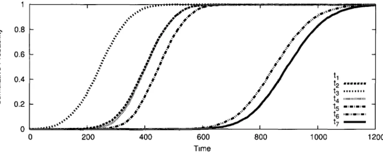
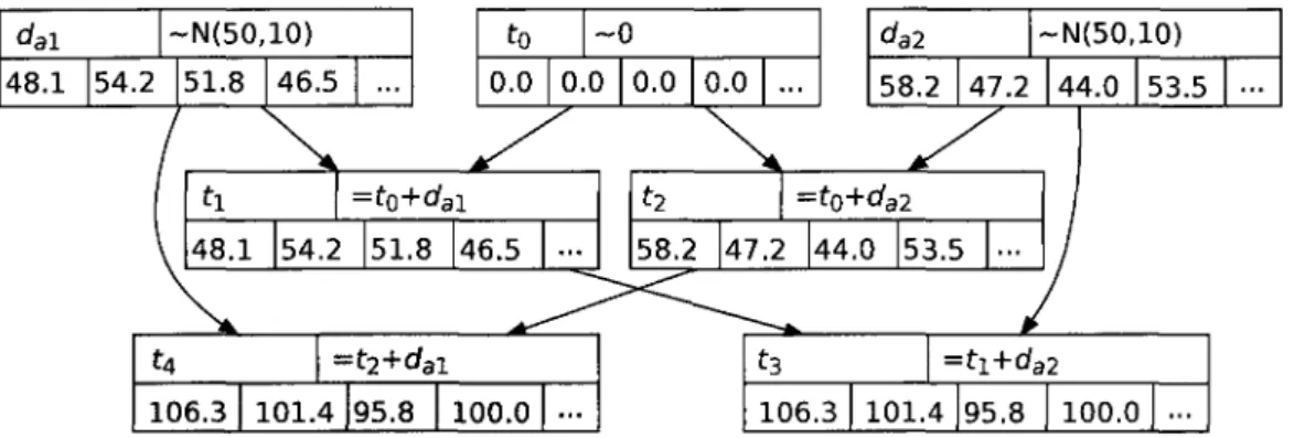
1.6 Extracted nonconditional plan 27 1.7 Random variables with samples 30 1.8 Estimated cumulative distribution functions (CDF) of random variables 31
1.9 Sample Bayesian network with equations in original and canonical forms 38 1.10 Bayesian network with arrays of samples attached to random variables 39
1.11 Example with two goals 41 1.12 Possible nonconditional plans 42 1.13 Possible actions in state S2 42 1.14 Latest times for starting actions 43 1.15 Example of time conditioning 53 1.16 Example of conditional plan 53 1.17 Impact of number of samples 57
1.18 Impact of cache size 58 1.19 Classification of planning problems with actions concurrency and
un-certainty 59 2.1 Example of a map to explore 69
2.2 Example of a Bayesian network to model time uncertainty 70
L I S T E DES FIGURES
2.4 Example of quantum states 78 2.5 Example of an observation of a state variable 80
2.6 Example of expanded quantum state space 82 2.7 Example of expanded Bayesian network 82
2.8 Values of actions in a state q 84 3.1 Occupancy grid in a robot motion planning domain 94
3.2 Simple board for the Snakes and Ladders game 97 3.3 Performance improvement of an optimized policy generator 100
3.4 Simple board with an optimal single-player policy 100 3.5 Optimal policy to beat an opponent playing with an optimal policy to
reach the end of the board as quickly as possible 103 3.6 Required time to generate single- and two-players policies 105
3.7 Quality of plans as a function of the allotted planning time 107 4.1 The AZIMUT-3 platform in its wheeled configuration 116
4.2 ICR transition through a steering limitation 118 4.3 Different control zones (modes) induced by the steering constraints . 119
4.4 State parameters 120 4.5 Environments and time allocated for each query 127
4.6 Comparison of trajectories created by a random, a naive, and a biased
1.1 Actions specification of the Transport domain 18 1.2 Empirical results for Transport and Rovers domains 56 1.3 Empirical results for the A C T U P L A N on the Transport domain . . . . 58
2.1 Actions specification for the Rovers domain 74 2.2 Empirical results on the Rovers domains 85 3.1 Empirical results for the value iteration algorithm on the board from
Figure 3.2 99 3.2 Percentage of wins between single- and two-players policies 104
3.3 Improvement when considering the abandonment model 107
4.1 Parameters used 127 4.2 Comparison of a naive algorithm and our proposed solution 128
Introduction
La prise de decision automatique represente une capacite fondamentale en intel-ligence artificielle (IA). Cette capacite est indispensable dans de nombreux systemes intelligents devant agir de fagon autonome, c'est-a-dire sans interventions externes, qu'elles soient humaines ou d'autres natures. Par exemple, un robot mobile doit prendre une multitude de decisions afin d'accomplir sa mission. Ses decisions peuvent se situer a plusieurs niveaux, comme de selectionner sa prochaine tache, de choisir sa prochaine destination, de trouver un chemin securitaire, et d'activer ses actionneurs et ses capteurs. De fagon similaire, les personnages animes dans les jeux videos doivent egalement adopter automatiquement des comportements qui contribuent a augmen-ter le realisme du jeu, et ce, dans l'ultime but d'agremenaugmen-ter I'experience de jeu des joueurs humains. D'autres applications, comme des systemes d'aide a la prise de
deci-sions, doivent proposer des actions et parfois meme les justifier a l'aide d'explications concises.
Fondamentalement, une decision implique le choix d'une action a prendre. Tout comme les humains qui sont responsables de leurs choix, done de leurs agissements, un agent intelligent est lui aussi responsable de ses decisions, done de ses actions. Cette lourde responsabilite implique le besoin d'evaluer et de raisonner sur les consequences de ses actions. Ce raisonnement est indispensable puisque les consequences d'une action peuvent avoir des implications considerables sur d'autres actions futures. Cela est d'autant plus important lorsque des actions ont des consequences subfiles qui peuvent retirer des possibilites a l'agent de facpn irreversible, ou impliquer des couts significatifs. Le probleme decisionnel devient nettement plus complexe lorsque les consequences des actions sont incertaines.
plusieurs options, c'est-a-dire differentes fagons d'agencer ses actions au fil du temps. Dans ce contexte precis, une option est fondamentalement un plan d'actions. De facon generale, I'existence de plusieurs options implique la capacite de les simuler a I'avance afin de retenir la meilleure option possible. Ainsi, le probleme de prise de decisions automatique peut etre vu comme un probleme de planification ou le meilleur plan d'actions est recherche. En d'autres mots, un agent intelligent doit soigneusement planifier ses actions afin d'agir de fagon rationnelle.
Puisque la planification necessite de connaitre les consequences des actions plani-fiees, un agent intelligent doit disposer d'un modele de lui-meme et de l'environnement dans lequel il evolue. Le monde reel etant d'une immense complexite, un modele fi-dele a la realite est generalement hors de portee en raison des ressources limitees en capacite de calcul et en memoire. Ainsi, des simplifications dans la modelisation sont incontournables. Ces simplifications se font a l'aide de differentes hypotheses de travail qui reduisent la complexite des problemes de planification. Cela permet de trouver des plans dans des delais raisonnables, done de prendre plus rapidement des decisions. En contrepartie, les hypotheses simplificatrices adoptees peuvent affecter, a la baisse, la qualite des decisions prises. Sans s'y limiter, les hypotheses couramment utilisees [51] sont :
- Observabilite totale. A tout instant, tout ce qui est requis d'etre connu sur le monde (l'environnement)* est connu. Par exemple, dans un domaine robotique, la position du robot pourrait etre reputee comme etant parfaitement connue a tout instant.
- Deterministe. Le resultat d'une action est unique et constant. En d'autres mots, il est presume que l'execution se deroule dans un monde parfait ou les actions ne peuvent pas echouer et que leurs effets sont totalement predetermines. - Monde statique. II n'y a pas d'evenements externes qui modifient le monde. - Plans sequentiels. Les plans sont des sequences d'actions ou chaque action
s'exe-cute l'une a la suite de l'autre. II n'y a pas d'actions concurrentes (simultanees). - Duree implicite. Les actions n'ont pas de duree, elles sont considerees comme
1. Dans cette these, les mots monde et environnement sont des quasi-synonymes. Dans la lit-terature, le mot monde (world en anglais) est generalement employe en planification en IA pour designer une simplification (un modele) de ce qui est appele environnement en IA et en robotique mobile.
INTRODUCTION
etant instantanees ou de duree unitaire au moment de la planification.
En combinant les hypotheses precedentes, plusieurs classes de problemes (et d'al-gorithmes) de planification sont creees : classique, deterministe, non deterministe, probabiliste, etc. Les frontieres entre ces classes ne sont pas toujours nettes et cer-taines se chevauchent. Chaque classe admet un ensemble de domaines de planification.
Essentiellement, les travaux de recherche en planification en IA consistent a conce-voir une solution, soit une combinaison d'algorithmes de planification, d'heuristiques et diverses strategies, pour resoudre des problemes d'une classe donnee. Cette solu-tion est intimement liee a un ensemble tres precis d'hypotheses simplificatrices qui sont soigneusement preselectionnees en fonction des applications ciblees. Le but est de trouver un juste compromis entre la qualite des decisions prises et les ressources necessaires en temps de calcul et en memoire. Ce defi est d'autant plus ambitieux considerant qu'une solution generale est hautement souhaitable. En d'autres mots, on desire une solution de planification qui est la plus independante possible de 1'ap-plication ciblee afin qu'elle soit facilement adaptable a de nouvelles ap1'ap-plications.
Au cours des dernieres annees, des progres considerables ont ete realises dans le domaine de la planification en IA. Pour certains types de problemes de planification, des planificateurs sont capables de generer efficacement des plans comprenant des centaines ou meme des milliers d'actions. Par contre, ces planificateurs sont souvent bases sur des hypotheses peu realistes ou tout simplement trop contraignantes pour etre utilises dans des applications reelles.
Cette these presente des avancees pour une classe de problemes de planification specifique, soit celle qui combine des actions concurrentes (simultanees) et de I'incer-titude. L'incertitude peut se manifester par differentes formes, comme sur la duree des actions, la consommation et la production de ressources (ex. : energie), et sur les effets des actions tels que leur reussite ou echec. Par son immense complexite, cette classe presente un important defi [17]. Ce type de problemes est motive par plusieurs applications concretes.
Un premier exemple d'application est la planification de taches pour des robots evoluant dans des environnements ou des humains sont presents. Ces robots doivent etre capables d'effectuer des actions simultanees, comme de se deplacer tout en ef-fectuant d'autres taches. lis font face a differentes incertitudes qui sont liees a la
dynamique de l'environnement et a la presence d'humains. Par exemple, suite aux participations aux AAAI Robot Challenge de 2005 et 2006 [49], une difficulte obser-ved fut la navigation dans des foules. Les capteurs etant obstrues, le robot avait de la difficulte a se localiser. En plus d'avoir a contourner des personnes, qui representent des obstacles mobiles, la difficulte a se localiser a rendu la vitesse de deplacement tres imprevisible. Les interactions humain-robot ont egalement cause des difficultes puisqu'elles ont aussi des durees incertaines. A cette epoque, le robot utilisait un pla-nificateur deterministe [8] integre dans une architecture de planification reactive [7]. Un parametre important du modele du planificateur etait la vitesse du robot. Une valeur trop optimiste (grande) pouvait entrainer des echecs au niveau du non-respect des contraintes temporelles, alors qu'une valeur trop prudente (petite) pouvait pou-vait occasionner le manque d'opportunites. Un planificateur considerant I'incertitude sur la duree des actions pourrait ameliorer la performance d'un tel robot.
Un deuxieme exemple d'application associee a cette classe est la planification des activites des robots (rovers) deployes sur Mars [17]. Les robots Spirit et Opportunity deployes par la NASA doivent effectuer des deplacements, prechauffer et initialiser leurs instruments de mesure, et acquerir des donnees et des images en plus et les transmettre vers la Terre. Pour augmenter leur efficacite, ces robots peuvent exe-cuter plusieurs actions simultanement. Ces robots sont sujets a differentes sources d'incertitudes. Par exemple, la duree et l'energie requises pour les deplacements sont incertaines. Les donnees acquises par les capteurs ont egalement une taille incertaine, ce qui a des impacts sur la duree des telechargements. Actuellement, les taches de ces robots sont soigneusement planifiees a l'aide de systemes de planification a initiatives mixtes [1] ou un programme guide un utilisateur humain dans la confection des plans. Des planificateurs plus sophistiques pourraient accroitre le rendement de ces robots. Les jeux videos representent un troisieme exemple d'application pouvant contenir des actions concurrentes et de I'incertitude. L'lA dans les jeux peut avoir a com-mander simultanement un groupe d'agents devant se comporter de fagon coordonnee. L'incertitude peut egalement se manifester de differentes fagons dans les jeux. Par exemple, le hasard est omnipresent dans les jeux de cartes et dans les jeux de plateau impliquant des lancers de des. Les jeux de strategies peuvent egalement contenir des actions ayant des effets stochastiques. Cela s'ajoute a une autre dimension importante
INTRODUCTION
des jeux, soit la presence d'un ou plusieurs adversaires. II ne s'agit plus uniquement d'evaluer la consequence de ses propres actions, mais egalement d'etre en mesure de contrer les actions de l'adversaire.
Les systemes d'aide a la decision sont d'autres applications pouvant contenir des actions simultanees avec des effets probabilistes. CORALS [13, 14] est un exemple de systeme d'aide a la decision, developpe pour la division Recherche et developpement pour la defense Canada, qui supportera les operateurs de navires deployes dans des regions dangereuses dans le cadre de missions humanitaires ou de maintien de la paix 2.
Les attaques ennemies pouvant etre rapides et coordonnees, les operateurs doivent reagir rapidement en utilisant plusieurs ressources de combats simultanement. Les actions sont egalement sujettes a differentes formes d'incertitude, la principale etant le taux de succes des armes qui depend de plusieurs facteurs.
Les contributions presentees dans cette these visent a ameliorer la qualite et la rapidite de la prise de decisions pour des applications combinant des actions concur-rentes sous incertitude. La these est composee de quatre chapitres, chacun presentant des contributions specifiques.
Le chapitre 1 presente le planificateur A C T U P L A N qui permet de resoudre des problemes de planification avec des actions concurrentes, et de I'incertitude et des contraintes sur le temps et les ressources. Une representation d'etats basee sur un modele continu du temps et des ressources est presentee. Contrairement aux ap-proches existantes, cela permet d'eviter une explosion de l'espace d'etats. L'incerti-tude sur le temps et les ressources est modelisee a l'aide de variables aleatoires conti-nues. Un reseau bayesien construit dynamiquement3 permet de modeliser la relation
entre les differentes variables. Des requetes d'inferences dans ce dernier permettent d'estimer la probability de succes et la qualite des plans generes. Un premier pla-nificateur, ACTUPLAN1 1 0, utilise un algorithme de recherche a chainage avant pour generer efficacement des plans non conditionnels qui sont quasi optimaux. Des plans non conditionnels sont des plans qui ne contiennent pas de branchements condition-nels qui modifient le deroulement de l'execution selon la duree effective des actions.
2. L'auteur de la these a participe au developpement des algorithm.es de planification du systeme CORALS, mais a l'exterieur du doctorat.
A C T U P L A N "0 est ensuite adapte pour generer plusieurs plans qui sont fusionnes en un plan conditionnel potentiellement meilleur. Les plans conditionnels sont construits en introduisant des branchements conditionnels qui modifie le deroulement de l'execution des plans selon des observations a l'execution. La principale observation consideree est la duree effective des actions executees. Par exemple, lorsque des actions s'executent plus rapidement que prevu, il devient possible de saisir des opportunites en modifiant les fagon de realiser le reste du plan.
Le chapitre 2 presente le planificateur Q U A N P L A N . II s'agit d'une generalisation a plusieurs formes d'incertitude. En plus de gerer I'incertitude sur le temps et les ressources, les effets incertains des actions sont egalement consideres. Une solution hybride, qui combine deux formalismes bien etablis en IA, est proposee. Un reseau bayesien est encore utilise pour prendre en charge I'incertitude sur la duree des actions tandis qu'un processus decisionnel markovien (MDP) s'occupe de I'incertitude sur les effets des actions. Afin de resoudre le defi de la concurrence d'actions sous incertitude, l'approche s'inspire des principes de la physique quantique. En effet, Q U A N P L A N
effectue une recherche dans un espace d'etats quantiques qui permet de modeliser des superpositions indeterminees d'etats.
Le chapitre 3 explore une application differente ou la concurrence d'actions se manifeste dans une situation d'adversite. L'lA devient un element de plus en plus incontournable dans les jeux. Le but etant d'agrementer le joueur humain, des idees sont proposees pour influencer la prise de decisions en ce sens. Au lieu d'optimiser les decisions pour gagner, des strategies sont presentees pour maximiser I'experience de jeu de l'adversaire.
Le chapitre 4 porte sur la planification de mouvements pour le robot AZIMUT-3. II s'agit d'une contribution complementaire aux trois premiers chapitres qui portent sur la planification d'actions concurrentes sous incertitude. En fait, dans les architectures robotiques, la planification des actions et des deplacements se fait generalement a l'aide de deux planificateurs distincts. Cependant, ces planificateurs collaborent : le premier decide de l'endroit ou aller, alors que le second decide du chemin ou de la trajectoire a emprunter. Comme indique plus haut, pour planifier, le planificateur d'actions a besoin de simuler les consequences des actions. Le robot AZIMUT-3, etant omnidirectionnel, peut se deplacer efficacement dans toutes les directions. Cela
INTRODUCTION
presente un avantage considerable. Or, pour generer un plan d'actions, le premier planificateur a besoin d'estimer la duree des deplacements. Une fagon d'estimer ces deplacements est de planifier des trajectoires.
La these se termine par une conclusion qui rappelle les objectifs et les principales contributions presentes. Des travaux futurs sont egalement proposes pour ameliorer I'applicabilite des algorithmes de planification presentes. Ces limites sont inherentes aux hypotheses simplificatrices requises par ces algorithmes.
Planification d'actions
concurrentes avec des contraintes
et de I'incertitude sur le temps et
les ressources
Resume
Les problemes de planification combinant des actions concurrentes (simul-tanees) en plus de contraintes et d'incertitude sur le temps et les ressources re-presentent une classe de problemes tres difficiles en intelligence artificielle. Les methodes existantes qui sont basees sur les processus decisionnels markoviens (MDP) doivent utiliser un modele discret pour la representation du temps et des ressources. Cette discretisation est problematique puisqu'elle provoque une explosion exponentielle de l'espace d'etats ainsi qu'un grand nombre de transi-tions. Ce chapitre presente A C T U P L A N , un planificateur base sur une nouvelle approche de planification qui utilise un modele continu plutot que discret afin d'eviter l'explosion de l'espace d'etats causee par la discretisation. L'incerti-tude sur le temps et les ressources est representee a l'aide de variables aleatoires continues qui sont organisees dans un reseau bayesien construit
dynamique-ment. Une representation d'etats augmentes associe ces variables aleatoires aux variables d'etat. Deux versions du planificateur A C T U P L A N sont
presen-tees. La premiere, nommee A C T U P L A N "0, genere des plans non conditionnels a l'aide d'un algorithme de recherche a chainage avant dans un espace d'etats augmentes. Les plans non conditionnels generes sont optimaux a une erreur pres. Les plans generes satisfont a un ensemble de contraintes dures telles que des contraintes temporelles sur les buts et un seuil fixe sur la probabilite de succes des plans. Le planificateur A C T U P L A N "0 est ensuite adapte afin de gene-rer un ensemble de plans non conditionnels qui sont caracterises par differents compromis entre leur cout et leur probabilite de succes. Ces plans non condi-tionnels sont fusionnes par le planificateur A C T U P L A N afin de construire un meilleur plan conditionnel qui retarde des decisions au moment de l'execution. Les branchements conditionnels de ces temps sont realises en conditionnant le temps. Des resultats empiriques sur des bancs d'essai classiques demontrent I'efficacite de l'approche.
Commentaires
L'article presente dans ce chapitre sera soumis au Journal of Artificial
In-telligence Research (JAIR). II represente la principale contribution de cette
these. Cet article approfondit deux articles precedemment publies et presentes a la vingtieme International Conference on Automated Planning and
Schedu-ling (ICAPS-2010) [9] et a la dix-neuvieme European Conference on Artificial Intelligence (ECAI-2010) [10]. L'article presente a ICAPS-2010 presente les
fondements de base derriere la nouvelle approche de planification proposee, c'est-a-dire la combinaison d'un planificateur a chainage avant avec un reseau bayesien pour la representation de I'incertitude sur le temps [9]. L'article pre-sente a ECAI-2010 generalise cette approche aux ressources continues [10]. En plus de detailler ces deux articles, Particle presente dans ce chapitre va plus loin. Une extention est faite a la planification conditionnel. Des plans condi-tionnels sont construits en fusionnant des plans generes par le planificateur non conditionnel. L'article a ete redige par Eric Beaudry sous la supervision de Froduald Kabanza et de Frangois Michaud.
Resource Constraints and Uncertainty
Eric Beaudry, Froduald Kabanza
Departement d'informatique, Universite de Sherbrooke, Sherbrooke, Quebec, Canada J1K 2R1
e r i c . b e a u d r y S u s h e r b r o o k e . c a , f r o d u a l d . k a b a n z a @ u s h e r b r o o k e . c a
Frangois Michaud
Departement de genie electrique et de genie informatique, Universite de Sherbrooke,
Sherbrooke, Quebec, Canada J1K 2R1 f r a n c o i s . m i c h a u d @ u s h e r b r o o k e . c a
A b s t r a c t
Planning with action concurrency under time and resource constraints and uncertainty represents a challenging class of planning problems in AI. Cur-rent probabilistic planning approaches relying on a discrete model of time and resources are limited by a blow-up of the search state-space and of the number of state transitions. This paper presents A C T U P L A N , a planner
based on a new planning approach which uses a continuous model of time and resources. The uncertainty on time and resources is represented by continuous random variables which are organized in a dynamically gener-ated Bayesian network. A first version of the planner, ACTUPLAN1 1 0, per-forms a forward-search in an augmented state-space to generate near op-timal nonconditional plans which are robust to uncertainty (threshold on the probability of success). ACTUPLAN1 1 0 is then adapted to generate a set of nonconditional plans which are characterized by different trade-offs be-tween their probability of success and their expected cost. A second version,
A C T U P L A N , builds a conditional plan with a lower expected cost by merging previously generated nonconditional plans. The branches are built by con-ditioning on the time. Empirical experimentation on standard benchmarks demonstrates the effectiveness of the approach.
1.1. INTRODUCTION
1.1 Introduction
Planning under time and resource constraints and uncertainty becomes a problem with a high computational complexity when the execution of concurrent (simultane-ous) actions is allowed. This particularly challenging problem is motivated by real-world applications. One such application is the planning of daily activities for the Mars rovers [17]. Since the surface of Mars is only partially known and locally uncer-tain, the duration of navigation tasks is usually unpredictable. The amount of energy consumed by effectors and produced by solar panels is also subject to uncertainty. The generation of optimal plans for Mars rovers thus requires the consideration of uncertainty at planning time.
Another application involving both concurrency and uncertainty is the task plan-ning for robots interacting with humans. From our experience at the AAAI Robot Challenge 2005 and 2006 [49], one difficulty we faced was the unpredictable dura-tion of the human-robot interacdura-tion acdura-tions. Navigating in a crowd is difficult and makes the navigation velocity unstable. To address uncertainty, we adopted several non-optimal strategies like reactive planning [7] and we used a conservative planning model for the duration of actions. A more appropriate approach would require to directly consider uncertainty during planning. There exist other applications such as transport logistics which also have to deal with simultaneous actions and uncertainty on time and resources [4, 21].
The class of planning problems involving both concurrency and uncertainty is also known as Concurrent Probabilistic Temporal Planning (CPTP) [47]. Most state-of-the-art approaches handling this class of problems are based on Markov Decision Processes (MDPs), which is not surprising since MDPs are a natural framework for decision-making under uncertainty. A CPTP problem can be translated into a Con-current MDP by using an interwoven state-space. Several methods have been devel-oped to generate optimal and sub-optimal policies [45, 43, 46, 47, 56].
An important assumption required by most of these approaches is the time align-ment of decision epochs in order to have a finite interwoven state-space. As these approaches use a discrete time and resources model, they are characterized by a huge state explosion. More specifically, in the search process, an action having an uncertain
duration produces several successor states each associated to different timestamps. Depending on the discretization granularity, this results in a considerable number of states and transitions. Thus, the scalability to larger problems is seriously limited by memory size and available time.
Simulation-based planning approaches represent an interesting alternative to pro-duce sub-optimal plans. An example of this approach is the Generate, Test and Debug (GTD) paradigm [64] which is based on the integration of a deterministic planner and a plan simulator. It generates an initial plan without taking uncertainty into account, which is then simulated using a probabilistic model to identify potential failure points. The plan is incrementally improved by successively adding contingencies to the gener-ated plan to address uncertainty. However, this method does not provide guaranties about optimality and completeness [46]. The Factored Policy Gradient (FPG) [18] is another planning approach based on policy-gradient methods borrowed from rein-forcement learning [61]. However, the scalability of FPG is also limited and it does not generate optimal plans.
Because current approaches are limited in scalability or are not optimal, there is a need for a new and better approach. This paper presents A C T U P L A N , a planner based on a different planning approach to address both concurrency and numerical uncertainty1. Instead of using an MDP, the presented approach uses a
determin-istic forward-search planner combined with a Bayesian network. Two versions of
A C T U P L A N are presented. The first planner one is A C T U P L A N "0 and generates non-conditional plans which are robust to numerical uncertainty, while using a continuous time model. More precisely, the uncertainty on the occurrences of events (the start and end time of actions) is modelled using continuous random variables, which are named time random variables in the rest of this paper. The probabilistic condi-tional dependencies between these variables are captured in a dynamically-generated Bayesian network. The state of resources (e.g., amount of energy or fuel) are also modelled by continuous random variables and are named numerical random variables and also added to the Bayesian network.
With this representation, ACTUPLAN1 1 0 performs a forward-search in an aug-1. In the rest of this paper, the expression numerical uncertainty is used to simply designate uncertainty on both time and continuous resources.
1.1. INTRODUCTION
mented state-space where state features are associated to random variables to mark their valid time or their belief. During the search, the Bayesian network is dynami-cally generated and the distributions of random variables are incrementally estimated. The probability of success and the expected cost of candidate plans are estimated by querying the Bayesian network. Generated nonconditional plans are near optimal in terms of expected cost (e.g., makespan) and have a probability of success greater than or equal to a given threshold. These plans are well suited for agents which are constrained to execute deterministic plans.
A C T U P L A N , the second planner, merges several nonconditional plans. The non-conditional planning algorithm is adapted to generate several nonnon-conditional plans which are characterized by different trade-offs between their probability of success and their expected cost. The resulting conditional plan has a lower cost and/or a higher probability of success than individual nonconditional plans. At execution time, the current observed time is tested in order to select the best execution path in the con-ditional plan. The switch conditions within the plan are built through an analysis of the estimated distribution probability of random variables. These plans are better suited for agents allowed to make decisions during execution. In fact, conditional plans are required to guarantee the optimal behaviour of agents under uncertainty because many decisions must be postponed to execution time.
This paper extends two previously published papers about planning with concur-rency under uncertainty on the duration of actions and on resources. The first one presented the basic concepts of our approach, i.e. the combination of a deterministic planner with a Bayesian network [9]. The second one generalized this approach to also consider uncertainty on continuous resources [10]. This paper goes further and presents a conditional planner generating plans which postpone some decisions to execution time in order to lower their cost.
The rest of this paper is organized as follows. Section 1.2 introduces the definition of important structures about states, actions, goals and plans. Section 1.3 introduces the nonconditional planning algorithm (ACTUPLAN1 1 0) and related concepts. Sec-tion 1.4 presents the condiSec-tional planning approach ( A C T U P L A N ) . Experiments are reported in Section 1.5. Section 1.6 discusses related works. We conclude with a summary of the contributions and ideas for future work.
1.2 Basic Concepts
The concepts presented herein are illustrated with examples based on the Trans-port domain taken from the International Planning Competition 2 of the International
Conference on Automated Planning and Scheduling. In that planning domain, which is simplified as much as possible to focus on important concepts, trucks have to de-liver packages. A package is either at a location or loaded onto a truck. There is no limit on the number of packages a truck can transport at the same time and on the number of trucks that can be parked at same location.
1.2.1 State Variables
State features are represented as state variables [53]. There are two types of state
variables: object variables and numerical variables. An object state variable x e X
describes a particular feature of the world state associated to a finite domain Dom(x). For instance, the location of a robot can be represented by an object variable whose domain is the set of all locations distributed over a map.
A numerical state variable y £ Y describes a numerical feature of the world state. A resource like the current energy level of a robot's battery is an example of a state numerical variable. Each numerical variable y has a valid domain of values
Dom(y) = [yrmn, Umax] where (ymin, Vmax) € M2. The set of all state variables is noted
Z = X U Y. A world state is an assignment of values to the state variables, while
action effects (state updates) are changes of variable values. It is assumed that no exogenous events take place; hence only planned actions cause state changes.
For instance, a planning problem in the Transport domain has the following ob-jects: a set of n trucks R = { r i , . . . , rn} , a set m of packages B = {b\,..., bm} and
a set of k locations L = {li,..., Ik} distributed over a map. The set of object state variables X = {Cr,Cb \ r e R,b € B} specifies the current location of trucks and
packages. The domain of object variables is defined as Dom(Cr) = L (Vr 6 R) and
Dom(Cb) = L U R (\/b e B). The set of numerical state variables Y = {Fr \ r € R}
specifies the current fuel level of trucks.
1.2. BASIC C O N C E P T S
1.2.2 Time and Numerical R a n d o m Variables
The uncertainty related to time and numerical resources is represented using con-tinuous random variables. A time random variable t ET marks the occurrence of an event, corresponding to either the start or the end of an action. An event induces a change of the values of a subset of state variables. The time random variable to £ T is reserved for the initial time, i.e., the time associated to all state variables in the initial world state. Each action a has a duration represented by a random variable
da. A time random variable t £ T is defined by an equation specifying the time at
which the associated event occurs. For instance, an action a starting at time t0 will
end at time ti, the latter being defined by the equation t\ = to + da.
Uncertainty on the values of numerical state variables is also modelled by random variables. Instead of crisp values, state variables have as values numerical random
variables. We note TV the set of all numerical random variables. A numerical random
variable is defined by an equation which specifies its relationship with other random variables. For instance, let y be a numerical state variable representing a particular resource. The corresponding value would be represented by a corresponding random variable, let's say n0 £ N. Let the random variable consatV represent the amount of
resource y consumed by action a. The execution of action a changes the current value of y to a new random variable n\ defined by the equation n\ = n0 — consa^y.
1.2.3 States
A state describes the current world state using a set of state features, that is, a set of value assignations for all state variables.
A state s is defined by s = (14, V, H, W) where:
- U is a total mapping function U : X —»• \JxeXDom(x) which retrieves the current
assigned value for each object variable x £ X such that U(x) £ Dom(x). - V is a total mapping function V : X —)• T which denotes the valid time at which
the assignation of variables X have become effective.
- 1Z is a total mapping function 1Z : X —>• T which indicates the release time on object state variables X which correspond to the latest time that over all conditions expire.
- W is a total mapping function W : Y ^ N which denotes the current belief of numerical variables Y.
The release times of object state variables are used to track over all conditions of actions. The time random variable t = TZ(x) means that a change of the object state variable x cannot be initiated before time t. The valid time of an object state variable is always before or equals to its release time, i.e., V(x) < 1Z(x)\/x £ X.
The valid time (V) and the release time (7Z) respectively correspond to the write-time and the read-write-time in Multiple-Timeline of SH0P2 planner [28], with the key difference here being that random variables are used instead of numerical values.
Hence, a state is not associated with a fixed timestamp as in a traditional approach for action concurrency [2]. Only numerical uncertainty is considered in this paper, i.e., there is no uncertainty about the values being assigned to object state variables. Uncertainty on object state variables is not handled because with do not address actions with uncertainty on their outcomes. Dealing with this kind of uncertainty is planned as future work. The only uncertainty on object state variables is about w h e n their assigned values become valid. The valid time V(x) models this uncertainty by mapping each object state variable to a corresponding time random variable.
Figure 1.1 illustrates an example of a state in the Transport domain. The left side (a) is illustrated using a graphical representation based on a topological map. The right side (b) presents state s0 in A C T U P L A N formalism. Two trucks rx and r2 are
respectively located at locations l\ and Z4. Package bi is loaded on r\ and package b2
is located at location l3. The valid time of all state variables is set to time t0.
1.2.4 Actions
The specification of actions follows the extensions introduced in PDDL 2.1 [31] for expressing temporal planning domains. The set of all actions is denoted by A. An
action a £ A is a tuple a=(name, cstart, coverall, estart, tend, enum, da) where :
- name is the name of the action;
- cstart is the set of at start conditions that must be satisfied at the beginning of the action;
1.2. B A S I C C O N C E P T S s0 X Crl Cr2 0,1 Q>2 y Frl Fr2 U(x)
h
U
rl '3 V(x) to to to to n{x) to to to to W(y) n0 "0(a) Graphical representation (b) State representation Figure 1.1: Example of a state for the Transport domain
duration of the action;
- estart and eend are respectively the sets of at start and at end effects on the state object variables;
- enum is the set of numerical effects on state numerical variables;
- and da £ D is the random variable which models the duration of the action.
A condition c is a Boolean expression over state variables. The function vars(c) —>
2X returns the set of all object state variables that are referenced by the condition c.
An object effect e — (x, exp) specifies the assignation of the value resulting from the evaluation of expression exp to the object state variable x. The expressions
conds(a) and effects(a) return, respectively, all conditions and all effects of action a. A numerical effect is either a change ec or an assignation ett. A numerical change
ec = (y, numchangea!y) specifies that the action changes (increases or decreases)
the numerical state variable y by the random variable numchangea>y. A numerical
assignation ea = (y,newvaray) specifies that the numerical state variable y is set to
the random variable newvaraty.
The set of action duration random variables is defined by D = {da | a £ A} where
A is the set of actions. A random variable da for an action follows a probability
dis-tribution specified by a probability density function 4>da : R+ —>• E+ and a cumulative
distribution function $d a : R+ -> [0,1].
1. state s satisfies all at start and over all conditions of a. A condition c £
conds(a) is satisfied in state s if c is satisfied by the current assigned values of
state variables of s.
2. All state numerical variables y £ Y are in a valid state, i.e., W(y) £ [ymin, yma
x\-Since the value of a numerical state variable is probabilistic, its validity is also probabilistic. The application of an action may thus cause a numerical state variable to become invalid. We denote P(W(y) £ Dom(y)) the probability that a numerical state variable y be in a valid state when its belief is modelled by a numerical random variable W(y) £ N.
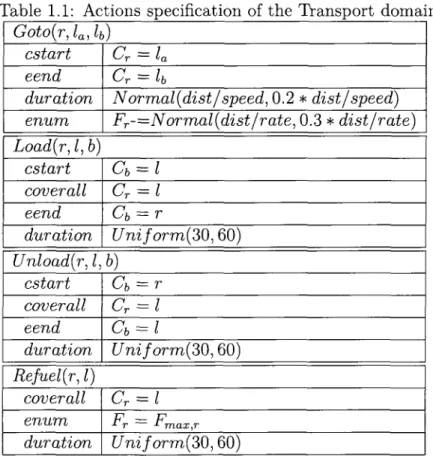
Table 1.1 presents actions for the Transport domain .
Table 1.1: Actions specification of the Transport domain
Goto(r, la,lb) cstart eend duration enum \jr — ia Cr = lb Normal(dist/speed, 0.2 * dist/speed) Fr-=Normal(dist/rate, 0.3 * dist /rate)
Load(r, I, b) cstart coverall eend duration Cb = l KJr := I Cb = r Uniform(30, 60) Unload(r, I, b) cstart coverall eend duration Cb = r C-v == I Cb = l Uniform(30, 60) Refuel(r, I) coverall enum duration C Y — I F = F x r •>• max,r Uniform(30, 60)
1.2. BASIC C O N C E P T S
1.2.5 Dependencies on Action Duration R a n d o m Variables
Bayesian networks provide a rich framework to model complex probabilistic depen-dencies between random variables [25]. Consequently, the use of continuous random variables organized in a Bayesian network provides a flexibility for modelling proba-bilistic dependencies between the durations of actions. Few assumptions about the independence or the dependence of durations are discussed in this section.The simplest case is to make the assumption that all actions have independent durations. Under the independence assumption, the duration of two arbitrary actions
a and b can be modelled by two independent random variables da and db. However,
this assumption may be not realistic for planning applications having actions with dependent durations. Let actions a and b represent the move of two trucks in traffic. If it is known that one truck is just following the other, it is reasonable to say that both actions should have approximately the same duration. This claim is possible because the uncertainty is not directly related to actions but to the path. This situation can be easily modelled in a Bayesian network by inserting an additional random variable
dpath which represents the duration of taking a particular path. Consequently, random
variables da and db directly depend on dpath.
Another important consideration concerns several executions of the same action. Let action a represent the action of moving a truck on an unknown path. Since the path is unknown, the duration of moving action is then probabilistic. Once the path is travelled for the first time, it may be reasonable to say that future travels along the same path will take approximately the same time. Hence we consider that if the duration of an execution of a is modelled by random variable da which follows the
normal distribution J\f(fx, a) 3 , executing action a twice has the total duration 2da
which follows A/"(2/u, 2a). It may also be the case that all executions of a same action have independent durations. For instance, the uncertainty about a may come from the traffic which is continuously changing. This can be modelled using one random variable per execution. Thus the total duration of two executions of a corresponds to
da,i + da£ which follows N(2/J,, \f2~o).
This discussion about dependence or independence assumptions on action
tion random variables can be generalized to the uncertainty on numerical resources. Depending on the planning domain, it is also possible to create random variables and dependencies between time and numerical random variables to model more precisely the relationship between the consumption and the production of resources and the duration of actions.
1.2.6 State Transition
Algorithm 1 A P P L Y action function
1. function A P P L Y ( S , a)
2. s' <- s
•3- tconds ^ ^•^^•x£vars(conds(a)) ^* ^V^-v 4- ^release ^ ^•^^•xEvars(effects(a)) S./CyX) £*• ^start * rnCLX\tcon(ls, ^release)
u- ^end * tstari -\- Ua
7. for each c e a.coverall 8. for each x e vars(c)
9. s'.1Z(x) <— max(s'.IZ(x), tenci)
10. for each e e a.estart 11. s'.U(e.x) <— eval(e.exp) 12. s'.V(e.x) <- tstart
13. s'.TZ(e.x) •<- tstart
14. for each e e a.eend
15. s'.U(e.x) <— eval(e.exp) 16. s'.V(e.x) <r- tend
17. s'.Tl(e.x) <- te n d 18. for each e e a.enum 19. s'.W(e.j/) «— eval(e.exp) 20. returns s'
The planning algorithm expands a search graph in the state space and dynamically generates a Bayesian network which contains random variables.
Algorithm 1 describes the A P P L Y function which computes the state resulting
from application of an action a to a state s. Time random variables are added to the Bayesian network when new states are generated. The start time of an action is defined as the earliest time at which its requirements are satisfied in the current state. Line 3 calculates the time tconds which is the earliest time at which all at start and over
1.2. BASIC C O N C E P T S
variables associated to the state variables referenced in the action's conditions. Line 4 calculates time treiease which is the earliest time at which all persistence conditions
are released on all state variables modified by an effect. Then at Line 5, the time random variable tstart is generated. Its defining equation is the max of all time random variables collected in Lines 3-4. Line 6 generates the time random variable tend with
the equation tend = tstart + da- Once generated, the time random variables tstart and
tend are added to the Bayesian network if they do not already exist. Lines 7-9 set the
release time to tena> for each state variable involved in an over all condition. Lines
10-17 process at start and at end effects. For each effect on a state variable, they assign this state variable a new value, set the valid and release times to tstart and add
tend- Line 18-19 process numerical effects.
Goto(rhlhl-2) Gotoir^l^l^ s0 X CA Crl Q l Cbl y Fr\ Frl U(x) h U ri h
my
V(x) h to 'o to K(x) to to to to ) "0 «0 — j Si X Crl Cr2 Q i ChZ y [Frl Frl U(X) h h r\ h V(X) h h k tonx)
h , to k to W(y) n\. "0 Sl X Crl Crl Cb\ Chi y Frl 'Frl u(x) k h ri hmy
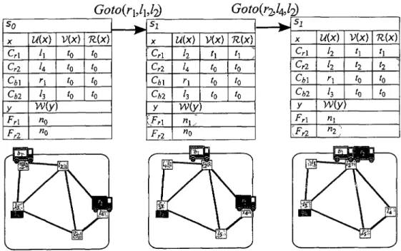
VU) 'l h to to KM h h ' to h ) nl n2]Figure 1.2: Example of two state transitions in the Transport domain
Figure 1.2 illustrates two state transitions. State si is obtained by applying the action Goto^lxM) f r o m s t a t e so- T n e A P P L Y function (see Algorithm 1) works
as follows. The action Goto(ri,ii,Z2) n a s t he at start condition Cn = h- Because
Cri is associated to to, we have tconds = max(i0) = *o- Since the action modifies
<faoto{rVlJ2) ~N(200,40) h =tl+dGoto(rl,llJ2) COnSGoto{r\,nj2) -N(2, 0.4) ^Goto(r2J4J2) ~N(400, 80) t2 =t0+dGoto{r2,tt,l2) COnSGoto(r2,l4,J2) ~N(4, 0.8)
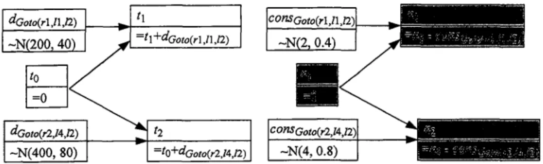
Figure 1.3: Example of a Bayesian network expanded after two state transitions
Line 5, the action's start time is defined as tstart = max(iconds, treiease) = to, which
already exists. Then, at Line 6, the time random variable tend = t0 + dGoto(rUh,i2) i s
created and added to the Bayesian network with the label t\. Figure 1.3 presents the corresponding Bayesian network. Next, Lines 13-16 apply effects by performing the assignation Cri = l? and by setting time ti as the valid time for Cri. The application
of the numerical effect creates a new numerical random variable n\ which is associated to the belief of FTl in state s\. As shown in the Bayesian network, nx is defined by
m = n0 - consGotoirauh) w n e r e conSGoto{rlth,h) is a random variable representing the
fuel consumption by the action. State s2 is obtained similarly by applying the action
Goto(r2,U,l2) from state si. Since both actions start at time t0, they are started
simultaneously.
1„2
07 G o a l s
A goal Q is a conjunction of deadline conditions over state features. A deadline condition is a tuple (x,v,dl) € Q meaning that state variable x e X has to be assigned the value v e Dom(x) within deadline dl € R+ time. In this paper, a goal is noted
by the syntax Q = {xl = vx@dW,... ,xn = vn@dln}. When a goal condition has no
deadline (dl = +oo), we simply write x = v, i.e. @dl = +oo is optional.
For a given state and goal, s (= G denotes that all conditions in G are satisfied in s. Because the time is uncertain, the satisfaction of a goal in a state (s \= G) is implicitly a Boolean random variable. Thus, P(s \= Q) denotes the probability that state s satisfies goal Q.
1.2. BASIC C O N C E P T S
actions may have a non-zero probability of infinite duration. For that reason, a goal is generally associated with a threshold a on the desired probability of success. Consequently, a planning problem is defined by (s0, Q, a) where so is the initial state.
1.2.8 Plans
A plan is a structured set of actions which can be executed by an agent. Two types of plans are distinguished in this paper. A nonconditional plan is a plan that cannot change the behaviour of the agent depending on its observations (e.g. the actual duration of actions). Contrary to a nonconditional plan, a conditional plan takes advantage of observations during execution. Hence, the behaviour of an agent can change according to the actual duration of actions. Generally, a conditional plan enables a better behaviour of an agent because it provides alternative ways to achieve its goals.
A nonconditional plan 7r is defined by a partially ordered set of actions IT =
(An, -<v) where:
- A^ is a set of labelled actions noted {labeli.ai,..., labeln:an} with a% e A; and
- <v is a set of precedence constraints, each one noted labelz -< . . . -< labelr
The definition of a plan requires labelled actions because an action can be executed more than one time in a plan. During execution, actions are executed as soon as their precedence constraints are satisfied.
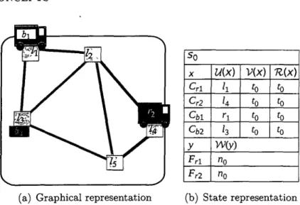
Let s0 be the initial state in Figure 1.4 and Q = {(Cbl = U)} be a goal to
satisfy. The plan n = ({ai: Goto(rx, li, Z2), a2. Unload(r\, l2, bi), a3: Go£o(r2, Z4, Z2),
a4: Load(r2,l2,bi), a5: Goto(r2,l2,l4), CL&: Unload(r2,l4,bi)}, {ax -< a2 -< a4, a3 -<
a4 -< a$ ^ a$ }) is a possible solution plan to the problem. This plan starts two
independent actions a\ and a^. Actions a2 is started as soon as a\ is finished. Once
both a2 and a% are finished, a4 is started. Finally, a5 and ae are executed sequentially
after a4.
A conditional plan w is defined as a finite state machine (FSM), where each state contains time switching conditions. In each state, an action is selected to be started depending on the current time which depends on how long the execution of previous actions have taken. A example of conditional plan and its construction are
so X Crl
c
r2 Q i O 2 y Frl Frl U(x)k
k
hh
V(x) to to to tonx)
to to to to W(y) "0 "o(a) Graphical representation (b) State representation
Figure 1.4: An initial state in the Transport domain
presented in Section 1.4.
The notation n (= Q is used to denote that the plan TT is a solution to reach a state which satisfies the goal Q.
1.2.9 Metrics
The quality of a plan n is evaluated by a given metric function cost(n). This evaluation is made from an implicit initial state s0- Typical cost functions are :
- the expected makespan denoted E[makespan(Tr)];
- the sum of the cost of actions;
- a formula evaluated on the last state s reached by the exection of n;
- or a linear combination of the expected makespan, the sum of the cost of actions and of a formula.
In this paper, makespan is used as the cost function for examples. The makespan of a plan ix is computed from the last state s which is reached by its execution and is evaluated by Equation (1.1). Note that the makespan of a plan is a random variable.
makespan(n) = maxs.V(x)
x£sC
1.3. ACTUPLANN C : NONCONDITIONAL PLANNER
1.3
A C T U P L A N
1 1 0: N o n c o n d i t i o n a l P l a n n e r
ACTUPLAN1 1 0 is the nonconditional planner version of A C T U P L A N . It performs a forward-search in the state space. A C T U P L A N handles actions' delayed effects, i.e. an effect specified to occur at a given point in time after the start of an action. The way the planner handles concurrency and delayed effects is slightly different from a traditional concurrency model such as the one used in TLPlan [2]. In this traditional model, a state is augmented with a timestamp and an event-queue (agenda) which contains delayed effects. A special advance-time action triggers the delayed effects whenever appropriate.
In A C T U P L A N , the time is not directly attached to states. As said in Section 1.2.3, A C T U P L A N adopts a strategy similar to Multiple-Timeline as in SHOP2 [52]. Time is not attached to states, it is rather associated with state features to mark their valid time. However, contrary to SHOP2, our planner manipulates continuous random variables instead of numerical timestamps. As a consequence, the planner does not need to manage an events-queue for delayed effects and the special advance-time action. The time increment is tracked by the time random variables attached to time features. A time random variable for a feature is updated by the application of an action only if the effect of the action changes the feature; the update reflects the delayed effect on the feature.
Algorithm 2 presents the planning algorithm of ACTUPLAN1 1 0 in a recursive form. This planning algorithm performs best-first-search 4 in the state space to find a state
which satisfies the goal with a probability of success higher than a given threshold a (Line 2). The a parameter is a constraint defined by the user and is set according to his fault tolerance. If s \= Q then a nonconditional plan n is built (Line 3) and returned (Line 4). The choice of an action a at Line 5 is a backtrack point. A heuristic function is involved to guide this choice (see Section 1.3.3). The optimization criteria is implicitly given by a given metric function cost (see Section 1.2.9). Line 6 applies the chosen action to the current state. At Line 7, an upper bound on the probability that state s can lead to a state which satisfies goal Q is evaluated. The symbol |=* is used to denote a goal may be reachable from a given state, i.e. their may exist a
plan. The symbol P denotes an upper bound on the probability of success. If that probability is under the fixed threshold a, the state s is pruned. Line 8 performs a recursive call.
Algorithm 2 Nonconditional planning algorithm 1. ACTUPLANnc(s, Q, A, a) 2. if P(s \=g)>a 3. n <— ExtractNonConditionalPlan(s) 4. return 7r 5. nondeterministically choose a € A 6. s' <- AppLY(s,a) 7. if P(s' K Q) > a 8. return A C T U P L A N "C( S ' , Q, A, a)
9. else return FAILURE
1.3.1 Example on Transport domain
Figure 1.5 illustrates an example of a partial search carried out by Algorithm 2 on a problem instance of the Transport domain. The goal in that example is defined by
Q = {Cbl — U}. Note that trucks can only travel on paths of its color. For instance,
truck r\ cannot move from Z2 to Z4. A subset of expanded states is shown in (a).
The states So, Si and s2 are the same as previous figures except that numerical state
variables, Fri and Fr2, are not presented to save space.
State S3 is obtained by applying Unload(ri,l2,b\) action from state s2. This
action has two conditions : the at start condition Cbl = r\ and the over all condition
Cri = h- The action has the at end Cbl = I2 effect. The start time of this action
is obtained by computing the maximum time of all valid times of state variables concerned by conditions and all release times of state variables concerned by effects. The start time is then max(£0,£i) = h. The end time is t3 = ti + dunioad(n,i2
M-Because the over all condition Cri = l2 exits, the release time lZ(Cri) is updated to
£3. This means that another action cannot move truck rx away from l2 before £3.
State s4 is obtained by applying Load(r2, l2,h) action from state s3. This action
has two conditions : the at start condition Cbl = l2 and the over all condition Cr2 = l2.
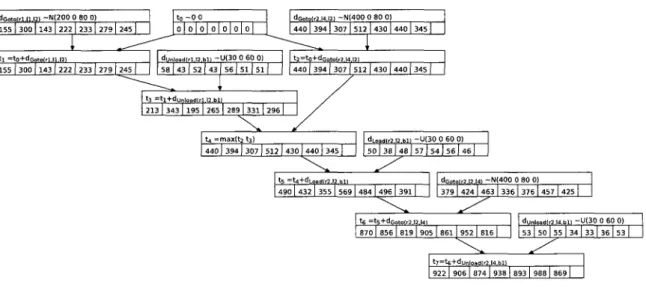
1.3. A C T U P L A NN C : NONCONDITIONAL P L A N N E R Goio{/\J\,lj) Goto^Wli) So X c„ C,: c„, Ca U{x) 1, 1. <•> /, V M <n k '» r0 K M '» '» '« 'o Unloaclir^.b^ Load^^) *1 X C,i Cr: Cn < K M M !•, 1, r, ' j V M f, 'o 'o In K M /, '» '» 'o <*Coro(rt,lU2) ~ N ( 2 0 0 . 80) '1 =fl+<fcoJo(rl /l /2) -'0^Col<i(rZ14)Z) S j x C i c« f»i C « WM I, I, r\ 1, V M /, ' ? '» 'o K M ' i ' 7 '» 'o * 3 X C,i c„ c« Ca K M 1, /, '» /, V M 1 K M /, 1 /J 'i h 'i 1 'i fo | 'o Gotofam * 4 X C",i c* C M C M WM ' i /, '1 1, V M i, ' 7 '< <0 K M ' 1 ' l '( 'o % X C,i Ca C M C K " M ' 7 1, ' 7 ;, V M 'i '« ' i 'o K M ' l ' I >0 Unload(r2,lt,b{) *s X crt c« C M C M K M 1 V M ' i ' , '4 >, '4 h '. 1 '» K M '. ' 7 ' 7 'o (a) State-space dunload(rl,ajil) ~U(30, 60) '3 ='l+<<t/7>taj<J(rl,/2,M) (b) Bayesian network
Figure 1.5: Sample search with the Transport domain
The end time is i5 = £4 + dLoad(r2,i2,bi)- The goal Q is finally satisfied in state s6.
Figure 1.6 shows the extracted nonconditional plan.