The influence of alley cropping systems on soil water dynamics and soil erosion in a changing climate.

(1)

THE INFLUENCE OF ALLEY CROPPING SYSTEMS ON

SOIL WATER DYNAMICS AND SOIL EROSION IN

A CHANGING CLIMATE

Scientific report for Ouranos-ICAR Climate Change Action Plan 26 “Biodiversity”

By Alain N. Rousseau Dennis W. Hallema Silvio J. Gumiere Gabriel Hould-Gosselin Claudie Ratté-Fortin

Centre Eau Terre et Environnement

Institut national de la recherche scientifique (INRS-ETE) 490, rue de la Couronne

Québec (QC) G1K 9A9

(2)

(3)

List of Tables

Table 1. MHYDAS-Erosion parameters ... 13

Table 2. Manning's roughness coefficient according to land use ... 14

Table 3. Saturated hydraulic conductivity according to soil type ... 15

Table 4:. Erosion parameter value ranges according to land use or soil type ... 16

Table 5. Particle size distribution (PSD) and organic matter for different depths below the alleyway of the experimental alley cropping site (analysis performed by M. Fossey). ... 19

Table 6. Particle size distribution (PSD) of the sand fraction for different depths below the alleyway of the experimental alley cropping site (analysis performed by M. Fossey). ... 20

Table 7. Monthly statistics calculated for 2011 and 2012 precipitation, average daily maximum (Tmax) and minimum (Tmin) temperature, and daily mean temperature at the experimental site. ... 23

Table 8. Land use and corresponding area cover. ... 30

Table 9. Soil types found in the micro-watershed. ... 31

Table 10. Monthly deltas and uncertainties of climate variables simulated for 2041-2070 for the southern part of Quebec with respect to 1971-2000 observations (Ouranos, 2012). The deltas were calculated with the constant scaling method and based on five different climate simulations, and are presented here as a change factor (-) or for temperature, as a change in centigrades. The statistically significant changes are underlined. ... 38

Table 11. Properties of the weather stations used for creating a reference dataset for St. Paulin. The last column indicates which data was used in the regression analysis and which data was used for creating the reference dataset. ... 39

Table 12. Values of soil hydraulic parameters (values based on Rawl et al., 1982). ... 42

Table 13. Hydraulic and distribution parameters of the root system with values based on Wesseling et al. (1991) (denoted *), Hinkley et al. (1994) (denoted **), Hadley et al. (2008) (denoted ***) and Bouttier (personal communication, denoted ****). ... 44

Table 14. Metrics used to evaluate the performance of simulations with MHYDAS-Erosion. ... 48

Table 15. Distribution and total precipitation for synthetic rainfall according to return period. ... 51

Table 16. Values of the alpha (shape) and beta (rate) parameters of the gamma distributions fitted to Ptot, Tmax and Tmin observed at St. Paulin in 2011-2012. ... 57

Table 17. Simulated 30-year statistics of daily precipitation, Tmax and Tmin for St. Paulin in 1967-1996. Values were estimated based on observation at Shawinigan, St. Charles de Mandeville and Quebec City airport. ... 62

Table 18. Rainfall characteristics for the 2012 events used in the calibration of MHYDAS-Erosion. ... 70

Table 19. Calibration metrics for the 19th of October ... 71

Table 20. Soil loss simulated with MHYDAS-Erosion for synthetic rainfall. ... 72

(7)

List of Figures

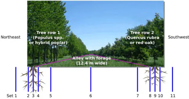
Figure 1. Springtime photograph of the experimental alley cropping site near St. Paulin, Quebec (31/05/2012). Tree rows are planted at a 12.4 m distance with an open space in between, the alley, where crops or forage are grown. The tree rows are not continuous in the row direction. 3 Figure 2. The water stress response function defined by (a) Feddes et al. (1978) and (b) Van

Genuchten (1987), adapted by Šimůnek et al. (2009). ... 8 Figure 3. Two-dimensional distribution of potential water uptake by roots represented with a

distribution function b(x,z) (Vrugt et al., 2001a,b). ... 9 Figure 4: Spatial discretization into surface units (SU) and reach segments (RS) performed with

PHYSITEL. ... 11 Figure 5: Topological links SU-SU & SU-RS at the micro-watershed’s outlet ... 12 Figure 6. The location of the St. Paulin experimental alley cropping site within Canada. ... 18 Figure 7. Satellite image of the experimental alley cropping site near St. Paulin, Quebec (marked with

the red frame; Cnes/Spot/Google). The NW-SE oriented lines within and below the indicated area are the alleyways with individual tree rows. ... 18 Figure 8. Fine root density of Quercus rubra (a) and Populus deltoides (b) as a function of depth below the surface and distance to the tree (Bouttier). ... 21 Figure 9. The weather station used at the experimental alley cropping site at St. Paulin, Quebec in 2011 and 2012 (picture taken on 23/05/2012). ... 22 Figure 10. Seasonal distribution of precipitation events observed in 2011 (a) and 2012 (b) at the

experimental site. ... 23 Figure 11. Wind roses calculated for the summer and autumn of 2011 (a) and 2012 (b) at one-minute

intervals, and the direction of wind gusts for 2011 (c) and 2012 (d). ... 24 Figure 12. Frequency domain reflectometer (FDR sensor) Onset S-SMB-M005 with UTP connector

cable. ... 25 Figure 13. Transect of the FDR setup at the experimental alley cropping site (diagram not drawn to

scale). ... 26 Figure 14. Plan view of the FDR setup at the experimental alley cropping site (not drawn to scale). The FDR sensors were divided into sets that are on a line perpendicular to the tree rows. Each set contains 2 to 5 sensors that monitor the volumetric water content at different depths: 7, 25, 45, 75 and 100 cm below the surface. ... 27 Figure 15. Satellite view of the micro-watershed at St-Narcisse-de-Beaurivage and its two main branches

... 28 Figure 16. Map of hydrological units (SU and RS) and land use ... 30 Figure 17. Sampling locations at the outlet of the micro-watershed. ... 32 Figure 18. Rating curve defining the relationship between water height and discharge at the catchment

(8)

Figure 22. Subdivision of the alley transect into three subdomains corresponding with the three vegetation types, which are from left to right Populus spp. (tree row 1), forage (alley) and

Quercus rubra (tree row 2) (diagram not drawn to scale). ... 41 Figure 23. Finite element mesh for the Populus spp. subdomain. ... 42 Figure 24. Material distribution for the Populus spp., forage and Quercus rubra subdomains with from

top to bottom loamy sand, sand, loam and clay loam (here shown for Populus spp.). ... 43 Figure 25. Linear interpolation of the soil moisture content on the starting date of scenario a

(03/06/2011). This interpolation was used as initial condition for the three subdomains (from left to right: Populus spp. between x=0-6 m, forage between x=6-18.4 m and Quercus rubra between 18.4-24.4 m). ... 45 Figure 26. Linear interpolation of the soil moisture content on the starting date of scenario b

(03/06/2012). This interpolation was used as initial condition for the subdomain of Populus

spp. ... 45 Figure 27. HYDRUS initial conditions for 2011 (a,b,c) and 2012 (d,e,f). ... 45 Figure 28: Tree strip locations according to topology for the hypothetical scenario. ... 50 Figure 29. A typical summer rainfall recorded in St. Paulin on August 10, 2011 (a), and the

corresponding soil water response over the course of 24 hours (b). ... 52 Figure 30. Linear (a) and Kriging interpolation (b) of volumetric water content to a depth of 100 cm

below Quercus rubra (red oak). The interpolated period is August 10, 2011 and shows rapid infiltration from point (1) to point (2), directly below the tree. ... 53 Figure 31. Distribution of 2012 daily precipitation at St. Paulin: (a) histogram and gamma probability

density function with alpha=0.61 and beta=0.08 fitted for P>0; (b) the quantile-quantile plot; (c) cumulative distribution functions; and (d) probability-probability plots. ... 54 Figure 32. Distribution of 2012 daily Tmax at St. Paulin: (a) histogram and gamma probability density

function with alpha=1593 and beta=5.41 fitted for P>0; (b) the quantile-quantile plot; (c) cumulative distribution functions; and (d) probability-probability plots. Note that temperature was converted to Kelvin in order to avoid negative values to which no gamma distribution can be fitted. ... 55 Figure 33. Distribution of 2012 daily Tmin at St. Paulin: (a) histogram and gamma probability density

function with alpha=2320 and beta=8.26 fitted for P>0; (b) the quantile-quantile plot; (c) cumulative distribution functions; and (d) probability-probability plots. Note that temperature was converted to Kelvin in order to avoid negative values to which no gamma distribution can be fitted. ... 56 Figure 34. Linear regression of cumulative precipitation (a), Tmax (b) and Tmin (c) observed at

Shawinigan (24 km NE of the experimental site) and St. Paulin in 2011. ... 58 Figure 35. Linear regression of cumulative precipitation (a), Tmax (b) and Tmin (c) observed at

Shawinigan (24 km NE of the experimental site) and St. Paulin in 2012. ... 58 Figure 36. Linear regression of cumulative precipitation (a), Tmax (b) and Tmin (c) observed at

Shawinigan (31 km WSW of the experimental site) and St. Paulin for the concatenated period 2011-06-01 to 2011-11-10 and 2012-04-24 to 2012-11-06. ... 58 Figure 37. Linear regression of cumulative precipitation (a), Tmax (b) and Tmin (c) observed at St.

Charles de Mandeville (31 km WSW of the experimental site) and St. Paulin in 2011. ... 60 Figure 38. Linear regression of cumulative precipitation (a), Tmax (b) and Tmin (c) observed at St.

(9)

Figure 39. Linear regression of cumulative precipitation (a), Tmax (b) and Tmin (c) observed at St. Charles de Mandeville (31 km WSW of the experimental site) and St. Paulin for the concatenated period 2011-06-01 to 2011-11-10 and 2012-04-24 to 2012-11-06. ... 60 Figure 40. Linear regression cumulative precipitation (a), Tmax (b) and Tmin (c) observed at Quebec

City airport (135 km ENE of the experimental site) and St. Paulin in 2011. ... 61 Figure 41. Linear regression of cumulative precipitation (a), Tmax (b) and Tmin (c) observed at Quebec City airport (135 km ENE of the experimental site) and St. Paulin in 2012. ... 61 Figure 42. Linear regression of cumulative precipitation (a), Tmax (b) and Tmin (c) observed at Quebec City airport (135 km ENE of the experimental site) and St. Paulin for the concatenated period 2011-06-01 to 2011-11-10 and 2012-04-24 to 2012-11-06. ... 61 Figure 43. (a) Simulated (line graph) and observed water content (circles) between 03/06/2011 and

03/11/2011 at a depth of 25 cm, 75 cm away from Populus spp. (in black; x=5.25 m) and at a depth of 25 cm directly below Populus spp. (in blue; x=6.0 m); (b) likewise for the period between 03/06/2012 and 03/11/2012. ... 63 Figure 44. Cumulative distributions of simulated pressure head in the summer and autumn of 2011 (top) and 2012 (bottom) for Populus spp. (a), forage (b) and Quercus rubra (c). The green lines mark the field capacity (pF=2) and wilting point (pF=4) between which water is available for plant roots... 64 Figure 45. Frequency of periods with waterlogging simulated for the period between 03/06/2011 and

03/11/2011 for Populus spp. (a), forage (b) and Quercus rubra (c), and dry periods for forage and Quercus spp. (d and e, respectively). The frequencies were calculated based on daily average water content at the specified locations. No dry days (pF>4.2) were simulated for

Populus spp. ... 65 Figure 46. Frequency of periods with waterlogging simulated for the period between 03/06/2012 and

03/11/2012 for Populus spp. (a), forage (b) and Quercus rubra (c), and dry periods for

Populus spp. (d). The frequencies were calculated based on daily average water content at the

specified locations. No dry days (pF>4.2) were simulated for forage and Quercus rubra. ... 66 Figure 47. Cumulative distributions of simulated pressure head between 03/06 and 03/11 of the year 2041 for Populus spp. (a), forage (b) and Quercus rubra (c). The green lines mark the field capacity (pF=2) and wilting point (pF=4) between which water is available for plant roots. Statistics were computed for a depth of 25 cm. ... 67 Figure 48. Cumulative distributions of simulated pressure head between 03/06 and 03/11 of the year

2071 for Populus spp. (a), forage (b) and Quercus rubra (c). The green lines mark the field capacity (pF=2) and wilting point (pF=4) between which water is available for plant roots. Statistics were computed for a depth of 25 cm. ... 67 Figure 49. Cumulative distributions of simulated pressure head between 03/06 and 03/11 of the reference period 1967-1996 (in black) and of the future period 2041-2070 (in blue) for Populus spp. (a), forage (b) and Quercus rubra (c). The green lines mark the field capacity (pF=2) and wilting

(10)

calculated based on daily average water content at the specified locations. No dry days (pF>4)

were simulated for Quercus rubra. Statistics were computed for a depth of 25 cm. ... 69

Figure 51. (a) Hydrograph separation and (b) model hydrological calibration for the 19th of October. .... 71

Figure 52. Flow rate (a and b) et simulated sediment flux at the outlet for a 6h Chicago distribution with a 10 year return period (right), and 24h Triangular distribution with a 100 year return period (left); without tree strips (c and d) and with tree strips (e and f). ... 73

Figure 53: Soil types surveyed by AAFC ... 90

Figure 54: Précision et exactitude des erreurs ... 93

Figure 55: TSS sampling apparatus ... 95

(11)

List of Abbreviations and Acronyms

BMP Beneficial management practice

CDF Cumulative distribution function

CRCM Canadian Regional Climate Model

DEM Digital Elevation Model

ET0 Reference evapotranspiration

FDR Frequency domain reflectometry

GCM Global climate model

INRS-ETE Institut National de la Recherche Scientifique – Centre Eau, Terre, Environnement

LIDAR Light detection and ranging

MHYDAS Modélisation Hydrologique Distribuée des Agrosystèmes

PET Potential evapotranspiration

PSD Particle size distribution

RCM Regional climate model

RS Reach segment

SCS Soil Conservation Service

(12)

1 Introduction

1.1 Framework

This study was conducted within the framework of the Climate Change Action Plan 26 “Biodiversity” funded by Ouranos and ICAR, under the supervision of A. Olivier (Université Laval) and in collaboration with partners at the UQAM Centre for Forest Research (A. Paquette and S. Domenicano), and Institut de Recherche en Biologie Végétale (UdeM; A. Cogliastro, D. Rivest and L. Bouttier).

Contributors at INRS were A. N. Rousseau (local project lead, research and field study), D. W. Hallema (hydrological research, field study, final report), S. J. Gumiere (research and field study, now at Université Laval), G. Hould Gosselin (research on erosion), C. Ratté-Fortin (rating curves), and in the field: G. Levrel (soil moisture probes), M. Fossey (grain size analysis), G. Carrer (meteorological station) and E. Maroy (all INRS-ETE). S. Tremblay (INRS-ETE) and Y. Périard (Université Laval) provided technical assistance.

1.2 The effects of alley cropping as an agroforestry practice

Alley cropping is an agroforestry practice whereby hardwood trees are planted at wide spacings, creating alleyways within which agricultural, horticultural or companion crops are grown (Gold and Garrett, 2009). In the temperate climate zone, alley cropping systems represent an alternative to traditional row cropping and help deal with specific issues such as wind erosion and crop failure due to excessive surface evaporation. The practice is also used in areas to help the transition of row crops into forest and for its excellent stewardship qualities (Garrett et al., 2011).

Hydrologists have long known that soil water dynamics and erosion by surface runoff depend in varying degrees on local weather (precipitation, solar irradiance, temperature and wind), vegetation (distribution of the root system, growth stage), soil characteristics (texture, soil type, porosity) and upstream drainage area. The implementation of alley cropping systems has an immediate effect on the first two in this list (local meteorological variables and vegetation), and studying these effects inescapably involves the study of the interaction between both.

1.3 Outline

The report continues with the scientific context and objectives. In the third chapter we will expand the theoretical framework within which we collected the required data and developed the corresponding methods (chapter 4). Chapter 5 and 6 present the outcomes of the study with most notably, the modeling results, followed by the conclusion in chapter 7.

(13)

2 Scientific context and objectives

2.1 Background

The components of a canopy of vegetation are known to influence the airflow near the land surface (Wilson and Shaw, 1977), and it is for this reason that alley cropping has a direct effect on transpiration and, as a consequence, on the soil water balance. Local meteorological variables are the result of an interaction between the thermal energy balance at the soil surface (net radiation, latent and sensible heat flux) and the atmospheric water balance (atmospheric density, vapor pressure deficit; Monteith, 1981).

Depending on characteristics of the environment in which alley cropping is practiced, such as elevation, relief and height of vegetation, we may expect that alley cropping systems influence local meteorological variables as well as the water distribution in the soil and at the soil surface. The distribution of soil water is a key factor in the growth and survival of trees and crops alike. If trees are able to redistribute water from layers with a low water availability (below the wilting point) to the upper layers of the soil where the trees and crops absorb water, both are more likely to survive and maintain high growth rates even during dry spells (e.g. Plamboeck et al., 1999).

Alley cropping also has an effect on erosion, depending on the type of crop. The cultivation of annual crops decreases the amount of soil organic matter, and can lead to enhanced erosion, especially on hillslopes with a high gradient (Kremer and Kussman, 2010). Perennial crops on the other hand maintain a continuous cover throughout the year, resulting in a reduced detachment of soil particles during rainfall and a maximization of infiltration. On the field scale, the tree rows may behave in a similar way as the vegetated filters along water streams, trapping sediment and preventing the evacuation of suspended load (Gumiere and Rousseau, 2011).

Given the reported effects of alley cropping in the microclimate zone, it is highly probable that alley cropping systems in southern Quebec provide a certain level of resilience to drought and increased rainfall intensity expected for this region (e.g. Mailhot et al., 2007), while simultaneously reducing the risk of water erosion and crop damage.

2.2 Objectives and hypotheses

In the light of changing environmental conditions caused by a shift in the local climate, the present study aims to characterize and evaluate local hydrology and erosion in an alley cropping system in southern Quebec for the present climate and climate conditions simulated for the period 2041-2070. Our

(14)

2.3 Approach

In order to quantify the effect of alley cropping systems on soil water dynamics and water erosion, we adopted a two-fold approach in which we study first the soil water dynamics, and second, the processes of water erosion, transportation and deposition, both for different climate change scenarios. The approach was divided into five steps, corresponding to five chapters of this report:

1. Field work: Collection of weather data, soil samples and soil moisture data during two field campaigns in 2011 and 2012 at an experimental alley cropping site near St. Paulin (province of Quebec, Canada) with two different tree species. Soil moisture patterns were measured with 45 frequency domain reflectometers (FDR sensors) installed up to a depth of one meter along a 25-m transect perpendicular to two tree rows and the alley between them.

2. Analysis of spatial patterns of water movement within the soil. The latter was done by performing a spatial interpolation of the point data obtained by the FDR sensors.

3. Analysis of weather data and simulation of climate change between the periods 1967-1996 and 2041-2070 at the experimental site. This step involves the simulation of daily values for precipitation, daily maximum temperature and daily minimum temperature.

Figure 1. Springtime photograph of the experimental alley cropping site near St. Paulin, Quebec (31/05/2012). Tree rows are planted at a 12.4 m distance with an open space in between, the alley, where crops or forage are grown. The tree rows are not continuous in the row direction.

The first three steps in the approach helped obtaining a first image of the hydrological processes that govern the alley cropping system, and the large number of FDR sensors installed on a small transect makes the field study unique in its own right. After data analysis we continued with:

(15)

4. Two-dimensional simulation of water movement within the soil below the alley cropping system. HYDRUS 2D/3D (Simunek et al., 1992) was used to describe the spatial domain of the transect with finite elements and simulate the following processes:

a. Variably saturated flow in the soil with the Richards equation (Richards, 1931);

b. Transpiration after root uptake with Feddes linear water stress response function (Feddes

et al., 1978; Feddes et al., 2001);

c. Potential transpiration using the Penman-Monteith equation (Penman, 1948; Monteith, 1981; Allen et al., 1998).

Three different scenarios were evaluated:

a. Scenario a: Observed field situation during the summer and autumn of 2011; b. Scenario b: Observed field situation during the summer and autumn of 2012; c. Scenario d: Climate change scenario for 2041-2070.

Scenarios a and b provide the parameterization of the model and are used to determine the water availability under current climate conditions, whereas scenario d gives an indication how alley cropping systems influence water availability to vegetation in the long term.

5. Simulation of the influence of the following processes on water erosion at the field scale with MHYDAS-Erosion (Gumiere et al., 2010): sheet erosion, rill erosion and sediment trapping by rows of trees in alley cropping systems. The modeling approach was divided in two steps:

a. Calibration of MHYDAS-Erosion on the 2.5-km2 Bras d’Henri microwatershed with intensive farming in the Beauce region of Quebec (study site of the Canadian project WEBs – Watershed Evaluation of Beneficial Management Practices); and

b. Simulation of the impact of alley cropping on sediment trapping at the same watershed using the parameter values found after calibration for synthetic rainfall events with return periods of 10, 50 and 100 year. Six- and 24-hour Chicago and triangular rainfall distributions were used to simulate the response to different rainfall peaks and average intensities, as these are the most common rainfall distributions in this region (Mailhot et

al., 2007). Two scenarios were evaluated for sediment trapping:

i. Bras d’Henri microwatershed without alley cropping (current field situation); and ii. Bras d’Henri microwatershed with alley cropping (hypothetical scenario). This

scenario assumes that tree rows are planted along the downstream edge of all fields.

(16)

3 Theoretical framework and literature review

3.1 Simulation of soil moisture patterns with HYDRUS 2D/3D

HYDRUS 2D/3D was selected as the software environment in which we developed a model for soil water movement below the alley cropping system. HYDRUS traces its roots to the SWMS_2D model (Šimůnek

et al., 1992; based on Van Genuchten, 1987), which later evolved into a software package for simulating

two- and three-dimensional movement of water, heat and solutes in variably saturated media (Šimůnek et

al., 2011; Šejna et al., 2011). The choice for HYDRUS 2D/3D was motivated by the versatility of the

software with respect to the spatial representation of the simulated domain and process interaction it can account for, and also by its widespread use for educational and professional applications.

The concepts and physically-based equations that represent hydrological processes within the model allow for simulating:

 Precipitation, infiltration, groundwater flow, throughflow and seepage using Richards equation (Richards, 1931);

 Transpiration after root uptake by vegetation using Feddes linear water stress response function (Feddes et al., 1978; Feddes et al., 2001);

 Evaporation from the soil surface and actual transpiration (together called evapotranspiration) using the Penman-Monteith equation (Penman, 1948; Monteith, 1981; Allen et al., 1998).

These governing equations have also been used in other physically-based models developed over the last decades. HYDRUS 2D/3D can simulate flow for different time scales (event-based or continuous-time) and spatial scales (soil column, plot scale and field scale). In this project we are mainly interested in soil water distribution at the plot scale, because this is the scale at which we can observe changes in local variables that play a role on the scale at which intervention takes place, namely the field scale.

The hydrologic response of an alley cropping system is characterized by the following hydrological processes. First rainfall infiltrates into the soil surface and from there moves vertically and laterally through the soil (infiltration, throughflow). This phenomenon is simulated using the Richards equation for variably saturated flow. Subsequently, water can be either stored in pore spaces, leave the upper soil by percolation to the groundwater table, be taken up by roots (potential transpiration), or evaporate directly from the soil surface.

We have selected three models that are able to simulate these processes observed in the soil (up to 1.5 m depth), which are (i) the nonlinear Richards equation for variably saturated flow in the soil, (ii) Feddes linear water stress response function for simulating water uptake by roots, and (iii) the Penman-Monteith evaporation model for surface evaporation.

(17)

3.1.1 Model for variably saturated flow

We used the Richards equation (Richards, 1931) to simulate infiltration and variably saturated flow in the soil. This is a non-linear partial differential equation that combines the Darcy-Buckingham equation and the continuity equation (formulated here for one dimension):

where θ is the volumetric water content [L3 L-3], t is time [T], z is a spatial coordinate [L], K(h) is the hydraulic conductivity, which is a function of pressure head h [LT-1], and S(h) is a sink function representing water uptake by roots. The formulation above is the mixed form of the Richards equation, referring to the presence of two dependent variables θ and h, where the rate of change in water content is expressed by the sum of the capillary flow and gravity flow terms minus the sink term.

When is represented by a soil water capacity function Cw(h) that characterizes the slope of the

retention curve, the Richards equation can also be expressed in terms of pressure head only. This way, we obtain the pressure head formulation:

HYDRUS uses the numerical finite element method to solve the Richards equation in space and the finite difference method to solve the Richards equation in time. Soil water capacity function Cw(h) is defined by

a hydraulic model, in this case the Brooks and Corey (1964) soil water retention function:

| | , 1/

1, 1/

and hydraulic conductivity function given by:

/

where Ks is the saturated hydraulic conductivity, α is the inverse of an empirical air-entry value, n is pore

size distribution index assumed for a given particle size distribution, l is a pore connectivity parameter (value assumed equal to 2.0 by Brooks and Corey, 1964), and Se is the effective water content defined as:

(18)

3.1.2 Root uptake model

Root uptake was simulated with the model developed by Feddes et al. (2001), which defines the maximum possible (i.e. potential) water extraction rate by plants Sp(z) [T

-1

] under optimal water availability integrated over rooting depth Droot as equal to the potential transpiration rate Tp [LT

-1

]. Sp for

depth z is given by the fraction of the root length density at depth z over the total root length density:

where the potential transpiration rate was simulated with the Penman-Monteith equation (see following sections). The influence of water stress on water extraction is expressed by a dimensionless stress response function of the pressure head yielding:

where S(z) is the actual flux density at depth z and α the dimensionless water stress response function for

which 0 1.

The water stress response function can be defined in multiple ways, for example with a linear function (Feddes et al.,1978), with a nonlinear water and osmotic stress response function (Van Genuchten, 1987), and even in combination with a time-variable root depth function (Verhulst-Pearl, 1838; Pearl and Reed, 1920). For the sake of parsimony we use the linear water stress response function (Feddes et al., 1978) in combination with a constant root distribution that does not evolve over time (Vrugt et al., 2001).

Water stress response is approximated by a continuous linear function α defined by four pressure head values, numbered h1 to h4 (see figure below). Water uptake is assumed zero for pressure heads higher than

the air-entry pressure h1 ( 2 for sand, 2.4 for silt and 2.5 for clay), also called the

anaeobiosis point, and for pressure heads lower than the permanent wilting point h4 ( 4.2 for sand,

silt and clay).

Between field capacity h2 and wilting point h3 the water uptake rate equals Sp when the water stress is

minimal, in which case 1. When the pressure head in the pore spaces is higher than wilting point

h3, Sp equals the potential transpiration rate Tp. In the event that the pressure head falls below the wilting

(19)

Figure 2. The water stress response function defined by (a) Feddes et al. (1978) and (b) Van Genuchten (1987), taken from Šimůnek et al. (2009).

3.1.3 Water uptake distribution model

Rather than simulating the uptake of individual roots, the potential water uptake is simulated by a potential water uptake distribution function. Following this approach, it is possible to represent a variety of different root systems of different vegetation with one potential water uptake distribution function. The time-invariant distribution of the root systems is described by a shape factor that defines the two-dimensional distribution of potential water uptake (Vrugt et al., 2001a,b):

, 1 1 | ∗ | | ∗ |

where , is the potential water uptake distribution function, where and are the maximum rooting length and maximum rooting depth, respectively, and are the distances from the origin of the plant at the surface in horizontal and vertical direction, respectively, px, x*, pz and z* are empirical

parameters used to ensure zero water uptake at z=Zm. x* and z* are called the radius and depth of

maximum intensity, respectively. The potential water uptake can now be calculated for a root zone with arbitrary shape (Vogel, 1987):

, where Tp [L T

-1

]is the potential transpiration rate and St is the diameter of the zone through which the

(20)

Figure 3. Two-dimensional distribution of potential water uptake by roots represented with a distribution function b(x,z) (Vrugt et al., 2001a,b).

3.1.4 Potential evapotranspiration models

Assuming that the potential evapotranspiration rate was dominated by the upward flux from vegetation canopy, we used the Penman-Monteith equation to calculate a reference evapotranspiration rate ET0 [LT

-1

] for 2011 and 2012 with data recorded by the local weather station (Penman ,1948; Monteith, 1981; Allen et al., 1998):

0.408∆ 900₂₇₃

Δ 1 0.34

where is the net incoming radiation at the crop surface [MJ.m-2day-1], calculated as twice the radiation measured with the PAR sensor, is the heat transfer into the soil [MJ.m-2day-1], is the atmospheric density [kg.m-3], is the specific heat of moist air [1.013 kJ.kg-1.°C-1], T is the mean daily air temperature at 2 m height [°C], u2 is the wind speed at 2 m height, is the vapor pressure at temperature

[kPa], is the actual vapor pressure [kPa], Δ is the slope of the vapor pressure curve [kPa.C-1] and is the psychrometric constant [kPa.°C-1]. Heat transfer into the soil ( ) is relatively small compared to the other terms for the summer and autumn periods in a humid continental climate, and was therefore neglected.

The weather data available for the periods 1967-1996 and 2041-2070 did not include all variables necessary to calculate the Penman-Monteith equation, so for this period we used the empirical Hargeaves equation defined as (Hargeaves, 1974):

where PET is potential evapotranspiration, MF is a tabulated monthly factor depending on latitude, T is the daily mean temperature (degrees Fahrenheit) and CH is a correction factor for when the 24-hour mean relative humidity exceeds 64 per cent.

(21)

3.2 Simulation of water erosion with MHYDAS-Erosion

3.2.1 Model overview

Intensive agriculture is often the cause of accelerated erosion with ablation rates many times higher than the rate of soil forming processes (pedogenesis). Water erosion is observed in most parts of the world, and some regions are more prone to erosion than others depending on vegetation type and density, as well as rainfall intensity and frequency.

In agricultural watersheds, Beneficial Management Practices (BMPs) are known to improve soil conservation and reduce sediment transport toward streams in the Quebec province (Quilbé et al., 2007; Rousseau et al., 2013). Structural BMPs such as alley cropping and other agroforestry practices in particular have the potential to modify flow paths and sediment connectivity in agricultural watersheds, thereby improving the overall sediment abatement at the watershed scale (Gumiere et al., 2010, 2012).

The evaluation of the potential impact of alley cropping would ideally require two fields that are exactly alike, except for the presence of rows of trees on one of them, or else the possibility to cut the trees from an existing alley cropping site and study the difference before and after. The complexity of the study would also require the distributed measurement of erosion, transport and deposition processes, which is a great challenge by itself. These means were not available for this project and thus, a physically-based modeling approach was used for estimating the potential impact of alley cropping on water erosion at the field scale. In addition, a modeling study of erosion on alley cropping applied in the context of this study can eventually be upscaled in order to assess the influence of structural BMPs on erosion at the watershed scale.

For this part of the study, we used MHYDAS-Erosion (Gumiere et al., 2010), an event and physically-based distributed model for linear erosion in agricultural watersheds, to simulate the following processes:

 Sheet erosion, which includes detachment by rain splash (Yann et al., 2008) and transportation by shallow overland flow (Zhang and Horn, 2001), corrected for the transport efficiency reduced by discontinuity of flow (Gumiere et al., 2010);

 Rill erosion, transport and deposition by unconfined concentrated flow (Foster et al., 1995);  Deposition of suspended material (or sediment trapping) at the base of the tree row due to an

increased drag force exerted by the trees on flow (Deletic, 2005).

Because MHYDAS-Erosion was developed according to the principle of parsimony, the number of parameters is limited. The main input variables are rainfall intensity, soil map, land use map and land

(22)

3.2.2 Spatial discretization and topology

MHYDAS-Erosion uses a spatial subdivision of the watershed into surface units (SU) and a segmentation of the drainage network into channel sections, or reach segments (RS) (Lagacherie et al., 2010). The surface units were created by intersection of spatial data including the digital elevation model, drainage network and the location of the spatial boundaries associated with fields, roads, units of the soil map and BMPs. Each surface unit is connected to the downstream end either to one surface unit (if there is one) or to one channel section (RS). The boundaries of spatial units are stored as vector shapes and may take virtually any geometrical form. Therefore, the model framework allows for adding spatial discontinuities such as BMPs (Gumiere et al., 2010).

We used PHYSITEL (Rousseau et al., 2011) and a 1-m digital elevation model or DEM (LIDAR) to create a subdivision into hillslopes by identifying the drainage network and calculating the accumulation matrix. Field maps are also used as spatial information to define the SUs. Hydrological short circuits are identified in the field, and are incorporated in the model to better define the topological links SU-SU and SU-RS. Figure 4 shows how spatial information layers are superposed to define the SUs. The drainage network is then separated into as many RS units as there are SU-RS connexions. In this study, the soil map is not used specifically for the spatial definition of SUs as the number of homogeneous regions would be too large. The soil map is instead used to assign the dominant soil type to the corresponding SU.

Figure 4: Spatial discretization into surface units (SU) and reach segments (RS) performed with PHYSITEL.

Drainage

network Hillslope map Field map

Hydrological units (SU and RS)

(23)

Topological links SU-SU and SU-RS are derived from specific hydrological path calculated using PHYSITEL. Adjustments are then made to include short circuits that cannot be identified by PHYSITEL alone with in situ observations. For example, a small culvert under a farm road allows one field to drain to another. Because the farm road is higher than the fields it divides, this connection is not identifiable with the pathways derived by the flow matrix alone. Figure 5 shows the downstream portion of the micro-catchment where branches 14 and 15 converge. SUs and RSs are identified by black and red numbers, respectively. The blue arrows indicate the topological pathways for each SU-SU and SU-RS connexion. For example, excess precipitation on SU 53 (located in the centre of the figure 5) flows to SU 36 under a farm road through a small culvert (diameter of approximately 10 cm). The combined flow of surface runoff and the contribution from the downstream SU 36 then flows to the drainage network, or the RS 8. This method allows the user to have greater control over the topological links in the model, allowing a more realistic scenario supported by field observations.

Branch 15

(24)

3.2.3 Parameterization

3.2.3.1 Erosion parameters

As MHYDAS-Erosion takes into account spatially distributed information to create homogenous units, each model input parameter can also be spatially distributed. Geometric SU and RS parameters such as average slope, as well as soil stability parameters can be drawn from the same spatially distributed information used to generate SUs and RSs (crops, tillage practices, etc.). The model also requires as inputs initial moisture contents (θi); as initial conditions based on the normalized antecedent precipitation

index (NAPI) for periods of 48 hours and 5 days. (Heggen, R. 2001). Table 1 shows the input parameters MHYDAS-erosion requires. Each parameter has a distinct value for each RS and SU.

Table 1 : MHYDAS-Erosion parameters

It should be noted that all hydrological and soil input parameters can vary during the year depending on land use (growth stage of crops, ploughing, etc.). The following sections explore in greater detail the range of values taken by each parameter according to land cover. A detailed look at the equations governing the transport and erosion mechanisms is beyond the scope of this report, and is presented in more detail by Gumiere et al. (2010).

(25)

3.2.3.2 Hydrological parameters

Hydrological input parameters include hydraulic conductivity (ks), air entry potential (hc), residual and

saturated moisture content (θs and θr) and Manning’s roughness coefficient for SUs and RS (nSU and nRS).

These parameters are mainly responsible in separating precipitation into surface and sub-surface flow, as well as surface flow velocities and heights.

The values chosen for the Manning’s coefficient are based on field observations throughout the summer and fall of 2012 and are based on the recommended values by Chow et al. (1964). Table 2 shows the different values assigned to the SU and RS as was growth or activity in the field.

Table 2: Manning's roughness coefficient according to land use (from Chow et al., 1964)

Occupation Manning start/end of season Manning mature Manning cut Manning plowed Unknown 0.03 0.035 0.03 0.030 Maize 0.032 0.040 0.032 0.027 Oats 0.032 0.450 0.032 0.030 Soy 0.030 0.040 0.035 0.027 Prairie 0.040 0.050 0.040 -

Prairie (late growth) 0.030 0.045 0.040 -

Forest 0.100 0.150 - -

(26)

Residual moisture and saturation moisture (θs and θr) are based on soil texture described in the soil map

provided by Agriculture and Agri-Food Canda (AAC) and corresponding values provided by the United States Department of Agriculture (USDA). Hydraulic conductivity values however, are not only strongly influenced by soil type, but also by farming practices such as ploughing. Coherent values for SUs and RSs are found by intersecting the soil and hydrological unit maps and assigning the dominant soil type for each unit. Those values are then altered if ploughing took place. Saturated hydraulic conductivity values (ks) for the untilled soils were surveyed by AAC and their values are reported in Table 3. For the same

ploughed soils, SU hydraulic conductivity values are multiplied by a factor of 10, as in situ measurements were not available.

Table 3: Saturated hydraulic conductivity according to soil type (see Table 9 for the nomenclature of soil names)

Soil ks (mm/h) Soil ks (mm/h) ALL 0.1 LBS 0.3 BVG1 19.6 MWO 21.1 BVG2 10.0 NUB 2.0 DGX 8.8 RRR 1.0 DQT 47.0 SJU 3.3 DSP 0.1 SPH 19.6 DSU 0.1 VAR 3.0

Finally, air entry potential values (hc) are linked to residual and saturation moisture as well as topsoil

porosity. Air entry potential values varying from 0.20 to 0.32 m are allocated by weighing a fixed maximum value (0.35 m) with topsoil porosity values surveyed by AAFC in 2007. .

3.2.3.3 Erosion and transport parameters

Parameters specific to the erosion and sediment transport alter soil cohesion, transport and deposition properties. MHYDAS-erosion simulates these processes in two parts: process caused by the impact of raindrops between the rills, and process caused by concentrated surface flow within the rills. Rills are defined as preferential paths, naturally formed by the topography, or artificially by ploughing.

Processes affecting the detachment and transport by rainfall only take place on SUs and are mainly contained in the areas between the rills. The interrill detachment equation used to simulate these processes was developed empirically by Yan et al. (2008) initially for the ultisoils type in China. Parameters influencing these processes can be summarized as: soil aggregate stability index between the rills (As) and

transport efficiency coefficient between rills (CETI). The concept of CETI was introduced to describe the effect of the perpendicular roughness on the interrill-to-rill erosion contribution. CETImax is the maximum

value that CETI can take.

Sediment detachment and transport processes in surface flow take place within SU rills and within the drainage network (RS). Parameters used in these processes can be summarised as: rill erodibility (Kr) and

(27)

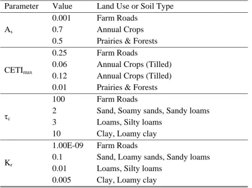
Value ranges suggested by Gumiere et al. (2010) for each parameter are attributed to each SUs or RS according to land use and soil type. Erosion parameter value ranges are set according to land use or soil type (see table below).

Table 4: Erosion parameter value ranges according to land use or soil type

Parameter Value Land Use or Soil Type

As

0.001 Farm Roads

0.7 Annual Crops

0.5 Prairies & Forests

CETImax

0.25 Farm Roads

0.06 Annual Crops (Tilled) 0.12 Annual Crops (Tilled) 0.01 Prairies & Forests

τc

100 Farm Roads

2 Sand, Soamy sands, Sandy loams

3 Loams, Silty loams

10 Clay, Loamy clay

Kr

1.00E-09 Farm Roads

0.1 Sand, Loamy sands, Sandy loams

0.01 Loams, Silty loams

0.005 Clay, Loamy clay

The number of rills per SU (Nrill) is limited to 30 to ensure model stability. As all SUs cover an area large

enough for more than 30 rills to occur, the maximum number of rills is attributed to all surface units in the watershed. Rill width is derived according to in situ observation and the crop type. For example, naturally occurring rills are distributed irregularly and have a width ranging between 10 and 50 cm. Artificial rills in corn fields are regularly spaced and have a width ranging from 60 to 75 cm. Finally, according to the sensitivity analysis performed by Gumiere et al. (2010), the median diameter of particles does not have a significant impact on simulation results, and is set to 0.3 mm.

(28)

4 Materials and methods

4.1 Materials

4.1.1 Description of the experimental alley cropping site

We selected an alley cropping site in the Rivière du Loup-Lac Saint-Pierre watershed near St. Paulin, Quebec, 20 km from the St. Lawrence River on the north shore at 46°27'9" N 72°59'29" W (see figure below). The site with an elevation between 130-144 m is located on Juneau Island, locked between two branches of the Rivière du Loup that split 1 km downstream of Hunterstown and merge again 600 m before the “Chute aux Chaudières” waterfall. The east bank (altitude 200 m) is an alluvial terrace with sand and gravel, whereas the west bank (altitude 160 m) and Juneau Island are characterised by loamy and clayey marine deposits, which were deposited when the region was covered by what is known as the Champlain Sea. The river bed is cut into the marine deposits to an altitude of around 125 m at Juneau Island, which is around 17-18 m lower with respect to the experimental site.

This site was selected for two reasons: (1) the site has an alley cropping system typical of the temperate climate zone, with hardwood trees planted at wide spacings and alleyways where agricultural, horticultural or companion crops are grown (Gold and Garrett, 2009); and (2) the alley cropping system was already an active research site for research on the contribution of multifunctional agroforestry systems to the climate change adaptation capacity of agro-ecosystems (professor Alain Olivier, Laval University).

The experimental alley cropping site is composed of a tree row with Populus spp. (hybrid poplar), another tree row with Quercus rubra (red oak), both planted in 2009, and within the alleyway Phleum pratense L. (common timothy) and Trifolium pratense L. (red clover), sown simultaneously in 2009. The alleyways are oriented NW-SE and are clearly visible in high resolution remote sensing imagery (figure below).

(29)

Figure 6. The location of the St. Paulin experimental alley cropping site within Canada.

Figure 7. Satellite image of the experimental alley cropping site near St. Paulin, Quebec (marked with the red frame; Cnes/Spot/Google). The NW-SE oriented lines within and below the indicated area are the alleyways with individual tree rows.

(30)

4.1.2 Particle size distribution (PSD)

An initial study was carried out by Bambrick et al. (2010) to determine the soil characteristics at the experimental site. They analyzed soil samples from one sample block in the western section of the field close to the Rivière du Loup, and found fractions of 79% sand by weight, 16% silt, 5% clay and pockets of sandy loam (56% sand, 30% silt and 14% clay). The soil was classified in situ as a dytric brunisol with pH 6.2 and moderate agricultural potential according to the Canadian Soils Classification System (Soil Classification Working Group, 1998).

In order to obtain the particle size distribution necessary for simulating the hydrology of the unsaturated zone at the experimental site, we extracted soil samples from within the alleyway, and assumed these were representative of the alley cropping system. The grain size analysis was based on the ASTM D-322 method (American National Standard Institute, 1972), as described by the Canadian Soil Survey Committee (McKeague, 1978). This method commends the dry sieving of the sand fraction precipitated after suspension. The organic matter content was determined by loss on ignition (LOI) at 375°C, as described by the Centre d'Expertise en Analyse Environnementale du Quebec. The particle size distribution, texture classes and organic matter content are given in the two tables below. Above a depth of 75 cm the soil is mostly sandy (up to 87-96% by weight) with smaller amounts of silt (2-8%) and clay (2-5%), which corresponds with the sandy soils found in this area by Bambrick et al. (2010). A clay loam layer below 110 cm contains up to 34% clay, which has a reducing effect on hydraulic conductivity. Organic matter content was highest within the first 35 cm below the surface (2.9-3.6 %).

Table 5. Particle size distribution (PSD) and organic matter for different depths below the alleyway of the experimental alley cropping site (analysis performed by M. Fossey).

Soil separates (% weight) Texture class Organic matter (% weight) Depth below surface (cm) Sand (0.05 - 1 mm) Silt (0.002 - 0.05 mm) Clay (< 0.002 mm) 0-15 87 8 5 Loamy sand 2.9 15-25 89 8 3 Sand 3.6 25-35 88 6 5 Sand 2.9 35-45 95 2 3 Sand 1.4 45-60 95 2 3 Sand 0.9 60-75 96 2 2 Sand 0.6 75-110 41 37 22 Loam 0.3 110-140 37 28 34 Clay loam 0.9

(31)

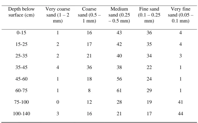
Table 6. Particle size distribution (PSD) of the sand fraction for different depths below the alleyway of the experimental alley cropping site (analysis performed by M. Fossey).

Soil separates (% weight)

Depth below surface (cm) Very coarse sand (1 – 2 mm) Coarse sand (0.5 – 1 mm) Medium sand (0.25 – 0.5 mm) Fine sand (0.1 – 0.25 mm) Very fine sand (0.05 – 0.1 mm) 0-15 1 16 43 36 4 15-25 2 17 42 35 4 25-35 2 21 40 34 3 35-45 4 36 38 22 1 45-60 1 18 56 24 1 60-75 1 8 61 29 1 75-100 0 12 28 19 41 100-140 3 16 21 17 44

4.1.3 Root distribution (Bouttier, 2013)

A parallel study was carried out within the framework of this project by Bouttier (2013) in order to determine the spatial distribution of the fine roots of Quercus rubra and Populus deltoides, the species planted in the tree rows, and of forage vegetation in the alley. The analysis was limited to the first 100 cm below the surface, because this is the zone where fine roots traditionally extract most water. The root systems of Quercus rubra L and forage are spatially separated, and the root density of Quercus rubra L at 0-10 cm depth is 17% lower than for forage, but 22% higher at a depth of 10-20 cm. The high root density of Populus deltoides near the stem results in a 45% lower root density for forage in those locations, which suggests strong competition for water resources between these two types of vegetation. The study of agricultural output has furthermore revealed a reduction of forage biomass especially near Populus

deltoides. Nevertheless, the results of a principal components analysis suggested that the effect of root

competition on agricultural output is only secondary, with competition for light being the principal factor of influence. The influence of the fast-growing Populus deltatoides root system on forage is greater than that of Quercus rubra L.

(32)

(a) (b)

Figure 8. Fine root density of Quercus rubra (a) and Populus deltoides (b) as a function of depth below the surface and distance to the tree (Bouttier).

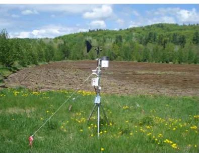
4.1.4 Weather data

A weather station (see figure below) was mounted in a suitable clearing at approximately 120 m from the alley cropping site (46°27'10.32"N 72°59'34.31"W) to measure air pressure, photosynthetically active radiation (400-700 nm), wind speed, wind direction, air temperature, relative humidity, and rainfall. Measurements were recorded every 15 minutes during the summer and autumn of 2011-2012. The following components were used to build the weather station:

 Monitoring: Independent monitoring system Onset Hobo U30 with space for a battery. This system operates under temperatures from -20 to 40 degrees C, has 10 Smart Sensor ports and 15 channels. Data are downloaded over a USB connection (mini-USB) using the Hoboware Pro software (Windows and MacOS). LEDs indicate system activity. Includes one 4 V 10.0 Ah battery (Power Sonic PS-4100).

 Power unit charged using one solar panel providing 1.2 W (Onset Solar).

 Relative humidity measurements: Onset S-THB-M002 Smart Sensor hygrometer for measuring relative humidity (1-100%) and temperature (-40 to 75 degrees C). Includes 2m cable.

 Wind speed and direction: Onset S-WCA-M003 combined anemometer and wind vane for wind speed between 0-44 m.s-1 and wind direction between 0-358 degrees (wind speed threshold of 0.5 m.s-1) mounted on an Onset M-CAB half cross arm attached to the tripod.

 Rain gauge: Onset S-RGB-M002 tipping bucket rain gauge (0.2 mm container), with 2 m cable.  Atmospheric pressure sensor: Onset S-BPB-CM50 Smart Sensor for measuring barometric

(33)

 Sensor for photosynthetically active radiation (PAR): Onset S-LIA-M003 sensor for visible light between 400-700 nm, includes 3 m cable.

 Solar radiation shield: Onset RS3, protects relative humidity and air temperature sensors.

 The weather station was mounted on an Onset M-TPB-KIT, which includes a 2 m metal tripod (M-TPB), a mast level (M-MLA), guy wire kit (M-GWA), 1/2” stake kit (M-SKA) for guy wires, 1/4” stake kit (M-SKB) for tripod and a grounding kit (M-GKA).

Figure 9. The weather station used at the experimental alley cropping site at St. Paulin, Quebec in 2011 and 2012 (picture taken on 23/05/2012).

The table below shows the monthly statistics of precipitation and temperature. The summer of 2012 was particularly dry in the province of Quebec, with precipitation as low as 32.4 mm in July against 95.4 mm in the same month a year before. August 2012 was still dry for the time of the year with 82.2 mm, but September and October were regular months. The contrast with 2011 is remarkable, here August was a very wet month with 188.2 mm, and the wettest day measured during the 2011field campaign was August 10, with 69.2 mm. The distribution of precipitation events in the figure below shows that October 2012 had the most days with precipitation. The wettest day of the 2012 field campaign also occurred in October (56.2 mm on October 31).

Daily mean temperature from July to October was very similar in 2011 and in 2012, while the daily range between minimum and maximum temperature was greater in 2012. The warmest temperatures were measured on July 22, 2011 (32.3°C) and on July 13, 2012 (34.5°C).

(34)

Table 7. Monthly statistics calculated for 2011 and 2012 precipitation, average daily maximum (Tmax) and minimum (Tmin) temperature, and daily mean temperature at the experimental site.

Date Precipitation (mm) Daily Tmax (°C) Daily Tmin (°C) Daily mean T (°C)

2011 2012 2011 2012 2011 2012 2011 2012 May - 63.2 - 20.0 - 6.5 - 13.5 June - 136.4 - 24.6 - 10.7 - 17.5 July 95.4 32.4 27.8 28.0 12.9 12.1 20.4 20.0 August 188.2 82.2 24.6 26.4 12.1 12.5 18.1 19.0 September 110.4 153.8 21.3 20.4 8.6 5.8 14.6 12.9 October 96.8 158.6 13.0 13.6 2.5 2.7 7.6 8.0 (a) (b)

Figure 10. Seasonal distribution of precipitation events observed in 2011 (a) and 2012 (b) at the experimental site.

The figure below shows the wind roses calculated for the summer and autumn of 2011 and 2012 at one-minute intervals (a and b), and the direction of wind gusts for the same periods (c and d). The wind came mostly from N to NNW (cold air) and from SSW (Saint-Lawrence Valley). Recorded wind speeds are quite slow compared to wind speeds observed in regions closer to the sea, and can be classified as gentle breeze at most (maximum wind speed 6 m.s-1, corresponding to Beaufort scale 3). Cold winds coming from NNW-NW were mostly light breezes with wind speeds up to 4 m.s-1 (Beaufort scale 2-3). Wind gusts coming from SSE-ESE were strongest, with speeds up to 15-16 m.s-1 (Beaufort scale 7).

(35)

(a) (b)

(c) (d)

Figure 11. Wind roses calculated for the summer and autumn of 2011 (a) and 2012 (b) at one-minute intervals, and the direction of wind gusts for 2011 (c) and 2012 (d).

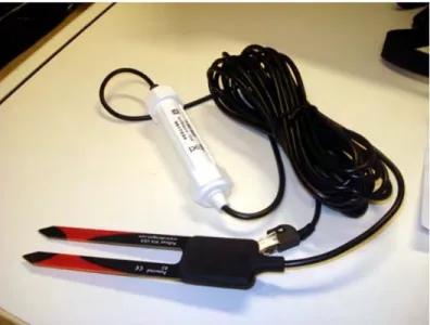
4.1.5 Soil moisture patterns measured with frequency domain reflectometry (FDR)

Forty-five frequency domain reflectometers of the type Onset S-SMD-M005 (see figure below) were used simultaneously to monitor volumetric water content within the first 100 cm of the soil along a transect perpendicular to the tree rows. The sensors were divided into 11 sets corresponding with a vertical profile, and inserted in the ground at depths of 7, 25 ,45, 75 and 100 cm (values correspond with the middle of the

(36)

Figure 12. Frequency domain reflectometer (FDR sensor) Onset S-SMB-M005 with UTP connector cable.

Each sensor has a unique frequency around 70 MHz, and the distance between two sensors within one set was chosen such as to avoid signal interference (>20 cm). The high frequency circuit also reduces sensitivity to salinity. This, together with the probe length of 10 cm being a few centimeters longer compared to other more sensitive sensors, helps averaging out any variability in soil moisture patterns within 1 dm3 of soil. The normal operation temperature of the sensors is between 0-50 degrees C. We used three independent Onset Hobo U30 monitoring systems. This system operates under temperatures from -20 to 40 degrees C, has 10 Smart Sensor ports and 15 channels. In combination with a Smart Sensor consolidator box and a power unit with a 85W solar panel and a deep cycle battery, it was possible to record the data of 45 FDRs with three monitoring systems. Data were sampled once per 15 minutes, based on the average value measured during the last minute of each 15 minute cycle. Data were downloaded over a USB connection (mini USB) using the Hoboware Pro software (Windows and MacOS). A LED indicates system status.

The sensors were installed as follows. First we drilled 45 holes in the ground using a hand auger with a 5 cm diameter. The shaft of each hole was cleaned during and after drilling using a soft brush. Subsequently, a metal rod with at one end an aluminum fork was used to pinch the soil at the bottom of the borehole in order to create room for the two pins of the probe. The FDR sensors were inserted vertically into the soil with the aid of a PVC tube in which we inserted the folded signal cable. Finally, the boreholes were filled with the same material that was removed before insertion.

(37)

(38)

Figure 14. Plan view of the FDR setup at the experimental alley cropping site (not drawn to scale). The FDR sensors were divided into sets that are on a line perpendicular to the tree rows. Each set contains 2 to 5 sensors that monitor the volumetric water content at different depths: 7, 25, 45, 75 and 100 cm below the surface.

(39)

4.1.6 Description of experimental micro-watershed used for calibrating the erosion model

The experimental micro-watershed (2.4 km2) used to calibrate the erosion model is a sub-watershed of the Bras d’Henri (150 km2), which is itself part of the Chaudière watershed in the south of the province of Quebec. The Bras d’Henri is intensively farmed with an animal density of 4.7 animal units per hectare of farmland, illustrating the importance of livestock farming in the area. Pig farming is practiced on 59% of agricultural units in the watershed, beef and poultry production, 23% and 6% respectively.

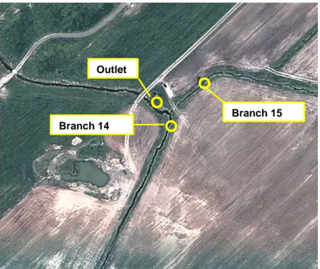
Figure 15 shows the micro-watershed, situated directly south-east of St-Narcisse-de-Beaurivage. The micro-watershed follows the Bras d’Henri’s trend in that it is intensively farmed, with very few wooded areas (mainly located south-west) covering 86% and 13 % of the total area, respectively. The remaining 3% consists of residential areas and farms located at the outskirt of the micro-watershed. Two main waterways separate the watershed drainage network, (branches 14 and 15) and converge at the outlet

Figure 15. Satellite view of the micro-watershed at St-Narcisse-de-Beaurivage and the two main creek branches

The micro-watershed is mainly used for large-scale farming practices including corn (20%), oats (6%), soy (31%) and prairies (24%) (year 2012). A large proportion of soy was farmed with residues left from previous growing seasons (18% with residues, 13% without), and 3% of prairies were planted late, exposing bare soil longer than other cultures.

Branche 15

Branche 14 Outlet

(40)

Table 8 shows the micro-watershed land cover in terms of area and percentage of use. Figure 21 shows the spatial distribution of land uses.

(41)

Table 8. Land use and corresponding area cover. Occupation (type) Area (km2) Occupation (%) Unclassified 0.09 4% Maize 0.50 20% Oats 0.14 6% Soy 0.33 13%

Soy (with residues) 0.45 18%

Prairies 0.52 21%

Prairie (late growth) 0.07 3%

Forest 0.32 13%

(42)

Soil types found at the surface are mainly limited to loamy sands and sandy loams. The table below shows the different types of soils and their properties, identified by a soil survey conducted in 2007 by AAFC. Finally, Appendix C provides a detailed soil map and specific to each type of soil found in the micro-watershed properties.

Table 9. Soil types found in the micro-watershed.

4.1.7 Data used for calibrating the erosion model

Calibration and validation require simulated and measured values of flow rates as well as sediment flux during several rainfall events. To this end, a measurement campaign during the major rainfall events of summer and fall 2012 was undertaken (from 4 July to 19 October 2012). For each rainfall event, precipitation, flow rate and total suspended solids (TSS) were recorded.

4.1.7.1 Rainfall

Precipitation was measured with a tipping bucket rain gauge installed on a weather station at the outskirts of the micro-catchment. Data was recorded continuously during the entire period of the measurement campaign. Monique Bernier’s team (INRS) operated the rain gauge used for this study. Data available at this station has an hourly resolution and were stored in a database via modem. According to previous uses of MHYDAS-Erosion, a one hour resolution is adequate to validate simulation results Gumiere et al. (2010).

(43)

4.1.7.2 Flow rate

As mentioned in section 4.1.6, two major branches run through the micro-catchment (branches 14 and 15) and meet near the outlet. Flow rates were measured at three sites, one downstream, and two upstream from the junction, respectively on branches 14 and 15. Mass balances between both branches and the outlet could be compared to check for consistency between measured results. In this report, only values reported for the outlet are discussed. Figure 17 shows the sampling location at the micro-catchment outlet.

Figure 17. Sampling locations at the outlet of the micro-watershed.

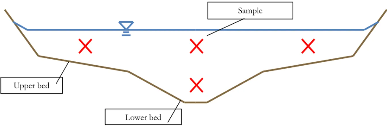
Flow rates were not measured directly, but were derived using a rating curve. This method involves the use of a regression curve between measured water heights in a channel with known dimensions, and measured flow rate. Unlike a hydraulic structures designed for this purpose such as a triangular weir, the measurement site is located in a natural section of the drainage network near the outlet, with a non-uniform section. Furthermore, the channel dimensions vary throughout the season depending on the stage of plant growth within the channel and sediment transport.

Manual measurements of flow rate and water level were taken every two weeks during the summer and fall periods by AAFC technicians. Following a preliminary analysis, we developed a regression function to establish the relationship between water level and flow rate (logarithm of a power function):

Branch 14 Outlet

(44)

season 2012. A detailed description of the method used to generate the rating curve can be found in Appendix D.

Figure 18. Rating curve defining the relationship between water height and discharge at the catchment outlet for the growth season of 2012

Water height was measured with an ultrasonic probe (Ultrasonic 710, see Figure 19). An average of the measured heights was recorded every 15 minutes during the measurement campaign. The ultrasonic module is attached to a metal frame directly above the riverbed.