Science Arts & Métiers (SAM)
is an open access repository that collects the work of Arts et Métiers Institute of Technology researchers and makes it freely available over the web where possible.
This is an author-deposited version published in: https://sam.ensam.eu Handle ID: .http://hdl.handle.net/10985/8216
To cite this version :
Patrick MARTIN, Jean-Yves DANTAN, Alain D'ACUNTO - Virtual manufacturing: prediction of work piece geometric quality by considering machine and set-up - International Journal of Computer Integrated Manufacturing - Vol. 24, n°7, p.610-626 - 2011
Any correspondence concerning this service should be sent to the repository Administrator : archiveouverte@ensam.eu
Virtual manufacturing: prediction of work piece geometric quality by conside ring machine and set-up accuracy
Patrick Martin*, JeanYves Dantan, Alain D’Acunto
LCFC, Arts et Métiers ParisTech,, 4 Augustin Fresnel 57078 Metz cedex3 France
Abstract: In the context of concurrent engineering, the design of the parts, the production planning and the manufacturing facility must be considered simultaneously. The design and development cycle can thus be reduced as manufacturing constraints are taken into account as early as possible. Thus, the design phase takes into account the manufacturing constraints as the customer requirements; more these constraints must not restrict the creativity of design. Also to facilitate the choice of the most suitable system for a specific process, Virtual Manufacturing is supplemented with developments of numerical computations (Altintas et al. 2005, Bianchi et al. 1996) in order to compare at low cost several solutions developed with several hypothesis without manufacturing of prototypes. In this context, the authors want to predict the work piece geometric more accurately by considering machine defects and work piece set-up, through the use of process simulation. A particular case study based on a 3 axis milling machine will be used here to illustrate the authors’ point of view. This study focuses on the following geometric defects: machine geometric errors, work piece positioning errors due to fixture system and part accuracy.
Keywords: virtual manufacturing; geometric error; machine tool; machining process; product-process integration
_____________________
Virtual manufacturing: prediction of work piece geometric quality by conside ring machine and set-up accuracy
Abstract: In the context of concurrent engineering, the design of the parts, the production planning and the manufacturing facility must be considered simultaneously. The design and development cycle can thus be reduced as manufacturing constraints are taken into account as early as possible. Thus, the design phase takes into account the manufacturing constraints as the customer requirements; more these constraints must not restrict the creativity of design. Also to facilitate the choice of the most suitable system for a specific process, Virtual Manufacturing is supplemented with developments of numerical computations (Altintas et al. 2005, Bianchi et al. 1996) in order to compare at low cost several solutions developed with several hypothesis without manufacturing of prototypes. In this context, the authors want to predict the work piece geometric more accurately by considering machine defects and work piece set-up, through the use of process simulation. A particular case study based on a 3 axis milling machine will be used here to illustrate the authors’ point of view. This study focuses on the following geometric defects: machine geometric errors, work piece positioning errors due to fixture system and part accuracy.
1. Introduction: virtual manufacturing
Nowadays, market fluctuation and trends require from the manufacturers a wide range of options and features for their products, but also decreased batch size, and reduced delays. The most effective answer to those market demands is the well-known concept of concurrent engineering (Sohlenius 1992).
The design of the parts, the production planning and the manufacturing facility must be considered simultaneously for this approach. This enables the design and development cycle to be reduced, with manufacturing constraints being taken into account as early as possible. Thus, the design phase takes into account the manufacturing constraints as the customer requirements; more these constraints must not restrict the creativity of design. Also to facilitate the choice of the most suitable system for a specific process, Virtual Manufacturing is supplemented with developments of numerical computations (Altintas et al. 2005, Bianchi et al. 1996) in order to compare at low cost several solutions developed with several hypothesis without manufacturing of prototypes.
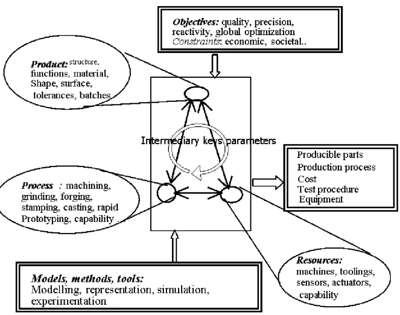
Our approach of product-process integration is illustrated in Figure 1: the quality of mechanical parts depends on the expression of specifications (shapes, functions, dimensions, surface quality and materials), the capacity of shaping processes and resource capability (defects in machine-tools, tools, fixtures). In order to fulfil these objectives, models and methods are used for manufacturing processes, designing production systems, validating product's manufacturability, defining the product qualification procedure. By process, we included all the operations and resources involved. That means that manufacturing processes (forging, casting, stamping, machining, assembling, fast prototyping…), production resources (machines, tools…), and conditions for implementation (setting and holding in position, operating conditions…), operation scheduling and the workshop lay-out can be take into account. Production constraints (process capability, producible shapes, precision...) must be taken into account at the same time as economic (cost...), logistics (lead-times, reactivity, size of production runs...) or legal (recycling, safety...) constraints. Knowledge and constraints must be structured, formalized and represented (data and processes).This information is derived from experimental data (product and resources) in industrial conditions. So, different types of expertise can be coherently integrated using appropriate models, methods and tools so as to meet production optimization objectives (quality, reactivity, productivity, cost…).
Figure 1: Reference diagram of product- process integration
Virtual prototyping is a design tool which supports the design process in the early stages and is used to minimize the associated risks before a large investment in continued development is made (Rogstrand et al. 2009, Samanta2009, Yang et al. 2006, Jun et al. 2005,). The early introduction of virtual prototypes will give designers and multidisciplinary teams greater freedom to exp lore compromises and the limiting values of a change or modification before it is actually implemented. In its most basic form, a virtual prototype will provide a three dimensional visualization that will enable the teams to establish a shared vision of the design and identify potential conflicts. With the addition of intelligent geometric reasoning, constraint management and dynamics simulation techniques, the virtual prototype becomes a very powerful interactive analysis tool. Computer-Aided Design (CAD) and the associated data are more and more used for visualizing, modelling, and simulating the manufacturing processes. As a result, digital manufacturing allows companies to develop
and test their manufacturing processes in a computer’s virtual environment – saving both development time and cost.
In this context we want to predict work piece geometric quality more accurately by considering machine limitations in the process simulation. We will particularly study a three axes milling machine. The scope of our work described in this paper is to focus on the following geometric defects:
- Machine geometric errors (axes straightness, parallelism errors…), - Positioning errors due to fixtures system.
We will consider numerical command errors and complex stresses as negligible factors. Elasticity of tool and machine bodies can be taken into account in the machine tool geometric error, elasticity of work piece can be introduced globally into the positioning error.
In fact classical approaches often neglect the parameters which influence part quality. For example, the milling process simulation typically considers that tools, machines, fixture elements and work pieces are perfectly rigid. It also assumes that the kinematics of machine joints is perfect. A more accurate analysis requires taking such machine errors into account. Mechanics, hydraulics and control units devices which are components of modern machine tool can introduce this kind of error...
When it comes to designing, each professional uses their own simulation programs (CAD, FEM software...), but an integrated design software of a complete machine system does not exist yet. For example, geometrical machine design, mechanical dynamics simulation and thermal analysis of the component use several kinds of software with different models with of the same product.
2. Geometrical tolerancing
The manufacturing industry has to improve the quality of its manufactured products, and this is the reason why industry needs tools and methods that allow predicting the product accuracy but that can also take into account of machine errors. There are several ways of improbing product quality:
- controling geometrical tolerances after manufacture, eliminating the bad parts or re-introducing the part which can be re-manufactured in the process,
- adjusting machine tools in order to respect best the functional requirements of the part, - controlling regularly the parts during production (SPC),
- simulating the geometrical effect of manufacturing fault causes and adjustment parameters with respect to the functional requirements.
2.1 The tolerancing task
We are here presenting some tools and methods that will allow us to improve the geometrical quality of the products by simulation of part manufacturing and kinematic joints of the machine tool. Then we will be able to link the value of adjustment parameters to the value of functional requirements, which will be applied to a part of a mechanism. In this way, we will be able to ensure the functional requirements are satisfied and to better estimate the value of adjustment parameters. In this context the authors want to predict more accurately the work piece geometric quality by considering the machine limitations through the use of process simulation with a particular case study based on a 3 axis milling machine. This paper will present our methodology approach and the tool used in order to meet to the geometrical requirements of a common mechanical part (about 10 micrometer of accuracy).
First, to understand the context and the problem, we should recall the definition of the tolerancing task. Tolerancing task is a part of the process design: it can be described as a subset of the geometrical definition of
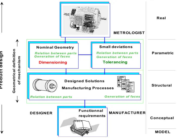
a mechanism. Product design aims at defining all the operations necessary to obtain real machine tool that meet optimal functional requirements (Martin and D’Acunto 2003). Limited to the geometrical point of view, product design demands two types of investigations.
Figure 2 : Geo metrical defin ition of mechanis m
- First, a structural study will consist in choosing design solutions and manufacturing processes that will allow the manufacturing of the mechanism. This mechanism is the answer to the functional requirements. Usually, the main aim of this study is to obtain technical documents which contain technical drawings, technical specifications, relevant information for manufacturing and all the calculation results. The latter describe the structure of the mechanism and consider all the links between parts and especially the different part set-up which allow to fix the part on the machine tool.
- Second, a parametric study analyzes and validates the result of the previous study for the developed mechanism.
Dimensioning and tolerancing are studied concurrently :
- dimensioning defines the nominal geometry. This description requires tools that describe and calculate geometrical dimensions of the part of the mechanism (computer aided design model),
- tolerancing deals with deviations between the acceptable geometry and the nominal geometry.
So the aim of tolerancing consists in controlling such deviations of a work piece in order to respect functional requirements.
If the control of deviations takes place during manufacturing and specific sensors are added on the machine, it can be possible to act directly on the machine tool controller. On the other hand, if we want to predict deviations before manufacturing, we have to carry out geometrical simulation. This s imulation needs part modelling tools that take into account tolerancing and dimensioning parameters. These dimensioning parameters appear in the manufactured faces process and in the machine structure.
2.2. Geometrical defects due to set-ups
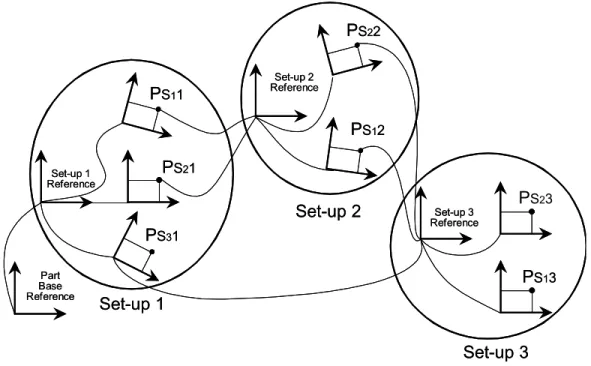
The machining process introduces geometrical defects due to the material’s behaviour, the deformations of tools or work pieces, as well as variations in cutting conditions. Moreover, in order to machine several faces of the work piece, several set-ups must be used (Figure 3). For each one, geometrical defects appear and they have to be added. These defects are identified experimentally on machined parts by using a tridimensional measuring machine. A machined surface (with its geometrical defects) in set –up 1 (figure 3) will become a reference face for the set-up 2 and so on. So the final machined feature (plane, hole, slot, 3D surface…) differ from each other, depending on the causes of manufacturing deviation and the numerous contact configurations in set-up. We introduce the manufactured point concept in order to predict the maximum deviation of the manufactured feature. This concept which results from observation of real machine tool, assumed that the parts are rigid (contact distortion and global distortion are disregarded). These parts (Figure 3) are in contact at the interface between a part and its fixtures at the time of manufacturing. This modeling allows the mechanism to be isostatic (as many equations as unknowns). In order to predict the accuracy of the work piece, the worst position for each set-up is taken into account. Thus, the accuracy will be predicted with common dimensions (a few hundred millimeters) of mechanical parts.
In general CAD software models work with the geometrical nominal values, and assume that the machine tools are geometrically perfect. The process planner needs to know the accuracy of the machine tools, the deviation caused by machining and set-up in order to define the process plan which allows to meet the work piece quality requirements. They can even add some finishing operation which increases the machining time and cost, in order to ensure the quality of the work piece.
3. Machine tool architecture
Models which describe the kinematics behaviour of a machine tool are proposed, taking into account the deviations of the kinematics joints and set-up. A set of mathematical and formal expressions constitutes the model and describes all the possible mechanisms in the machine tool.
Many works have been done to define and model the architecture of classical 3 to 5 axis machine tools (Reshetov and Portman 1988, Weck 1984, SME 1996, Bohez 2002), as well as new reconfigurable machine tool architecture, (Garro and Martin 1993, Koren et al. 1999, Shabakaet al. 2007, D’Acunto et al. 2007). In order to describe the position and the control of a kinematic chain of solids such as can be found in robotics, the homogeneous coordinates (matrix 4 x 4) are commonly used and are an efficient mathematical tool which can be easily manipulated thank to formal calculation tools. When the displacements are large, we use a formal expression of a rotation-translation matrix 4x4. This matrix introduces the parameter of displacement by building an expression of the nominal geometry. The 12 terms which are non zero or equal to1, characterize rotations (3 X 3 terms) and translations (last column).
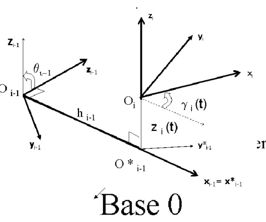
Each part i (figure 4) of the kinematics chain has an associated local axis system i. The position of i versus the previous component i-1 and its axis system i-1 is given by the product of position matrix Gi-1 (representing machine geometric structure) by Mi (representing the axis movement). For a classical machine tool structure, matrix Gi-1 [ i-1 │ i -1 * ] defines the architecture of the machine (position of the slides in terms of the axis origin position and angles between them), the movement matrix Mi [ i-1 *│ i ] has a single degree of freedom ( in translation X or Y or Z or in rotation A or B or C), i-1* is the intermediary axis system of the component i before moving. Positioning of the part feature on the one hand and the tool on the other hand can be directly calculated by one product of matrices (open chain of solids). The terms for machining are expressed by the identity of the 12 terms of the two matrices (equation (1)) for passing from base to feature and base to tool (Figure 4):
[Base │ Tool] equation (1) [Base │ n ] = 1,n G i-1 [ i-1 │ i -1 * ] * Mi [ i-1 *│ i ] equation (2)
Figure 4: Machine tool arch itecture
Thus, knowing the geometric and kinematic characteristics of each element, we can calculate the tool position in relation to the feature position, so an expression of the nominal geometry of the machine tool or
manufacturing system can be obtained. For the parts to be manufactured, information about the machining features, the machining sequences, the movements needed on each axis and their control type (point to point, paraxial, contouring), the possible accessibility directions (two directions for a n open hole, several directions for periphical milling…) have to be identified. Therefore, the CAD model has to be enriched with the relevant parameters for the machining process (Martin and D’Acunto 2003). From this information, the movements to be controlled by the numerical controller in order to manufacture the part on a classical machine tool or the architecture of the manufacturing system can be computed (Bohez 2002, Koren et al. 1999, D’Acunto et al. 2007).
Moreover, mechanical and manufacturing deviations are introduced. In fact, the machine architecture still has some geometrical defects (perpendicularity, parallelism, position…), the machine presents uncertainties in kinematic movements (gaps, deformations, yaw, pitch or roll deviations) and the part presents set-up deviations. For the normal accuracy class N (over a range of 5 classes), 22 errors on the machined work pieces caused by deviations of main geometrical accuracy parameters of machine tools have been identified (Reshetov and Portman 1988).
They are caused by:
- Radial and axial runout, - Linearity of sliding,
- Planeness of working surface, - Parallelism of working surfaces, - Perpendicularity of working surfaces, - Deviation of pitch.
The main defects of the workpiece are: - Nonroundness and non planeness,
- Non perpendicularity of hole axis to base plane,
- Non parallelism or non perpendicularity of machining surface, - Waviness of surfaces,
- Axial or radial play.
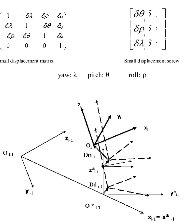
Works have been done to develop models for machine tool error (Reshetov and Portman 1988, Moon and Kota 2002, Tutenea-Fatan and Feng 2004, Ahn and Cho 1999, Eman and Wu 1987), for our purpose a model of machine tool deviations by homogeneous transformation matrix is used, so the same mathematical tool is used for modelling perfect and real machine. In the cases of small deviations, a linearised expression of the displacement can be used and a small displacement matrix (equation 3) which describes the small displacement screw is used. In this case it is very important to make a distinction between the defect due to machine tool architecture from the defect due to movement in the transformation matrix [ i-1 │ i ] in order to take into account each deviation in the virtual machining computation. For small values, the matrix can be linearised and becomes an anti-symetric matrix. This matrix represents the small deviation screw (Bourdet and Clément 1988) (Figure 5), which is a representation of the kinematic torsor {rotation vector│speed vector} applied to small displacement.
So equation 2 becomes:
[ O | n ] = 1 , n G i-1 * Dd i-1 * Mi * Dm i equation (3)
This procedure is an efficient framework for kinematic modelling and systematic design of re-configurable machine tools (D’Acunto et al. 2007, Moon and Kota 2002, Tutenea-Fatan and Feng 2004). This representation allows to capture the motion characteristics of machine components; it enables automatic selection of the machine tools as soon as the accuracy of each axis is known. The accuracy of machined part can be predicted by matrix multiplication (also called tolerance analysis). Moreover, if the accuracy of the part is given, computable operations such as matrix inversion and matrix multiplication allow to predict the accuracy needed for each kinematic joint (also called tolerance synthesis). It is a step towards development of an integrated tool for designing machine hardware and control schemes.
If we compare this work to other works dealing with the geometric error modelling for machine tools (Kyoung-Gee et al. 2005, Ahn and Cho 1999, Eman and Wu 1987, Chen 2000, Yao and al. 2006), our aim is to predict by simulation (virtual machining) the work piece errors made by machine tool accuracy which are experimentally identified, and set - up errors of the machined part.
4. Manufactured product geometry prediction
The goal here is to predict more accurately work piece geometric quality by considering machine limitations in the process simulation. We will particularly study a three axes milling machine. In the scope of our work, we will use the DELMIA® software (Dassault Systemes®), (a specific module is dedicated to design machine tool structure and kinematics) and focus on these geometric defects:
- Machine geometric errors (axes straightness, parallelism or perpendicularity errors, …), - Positioning errors due to fixture system.
These errors are estimated from sets of experiments.
We consider that the main defects result from these two errors, so we will neglect (second order defect) the following factors: controller errors, complex stresses, elasticity of work piece, tool and machine bodies. The dynamic characteristics of the machine tool or controller behaviour are not considered in this study. The main objective is to anticipate the work piece geometrical quality as soon as the geometrical deviation of each component and the kinematical joints defects are known or identified.
Detailed works have been done on the positioning errors and contact behaviour due to fixtures (Chaiprapat and Rujikietgumjorn 2008, Yeh and Liou 1999, Yeh and Liou 2000, Anotaipaiboon et al. 2006).
We consider that the part and the kinematic devices are rigid components, moreover the worst case that is maximum error of set-up error is considered.
In order to respond to this objective, the following tasks are completed: - Identifying a test part
- Identifying the machine tool, the geometrical defects and attribute mathematic functions to machine limitations
- Designing the virtual machine and assigning kinematics.
- Performing the simulation with and without including machine accuracy and set-up defects. - Analyzing results and observations.
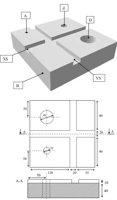
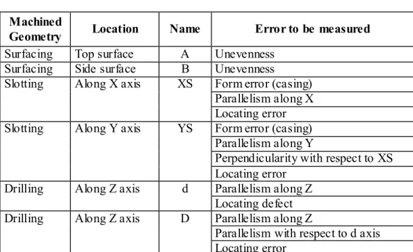
In order to observe the maximum amount of geometric errors on the work piece, we decided to design a test work piece with characteristic geometric forms (paralleled cylinder, perpendicular slots…) from which we could easily measure defects after machining.
Table 1 lists those simple geometries and associates the errors to be measured.
Figure 6 : Test part
Table 1 : Machining features and error to be measure
4.2. Identifying a machine tool and the geometrical defects
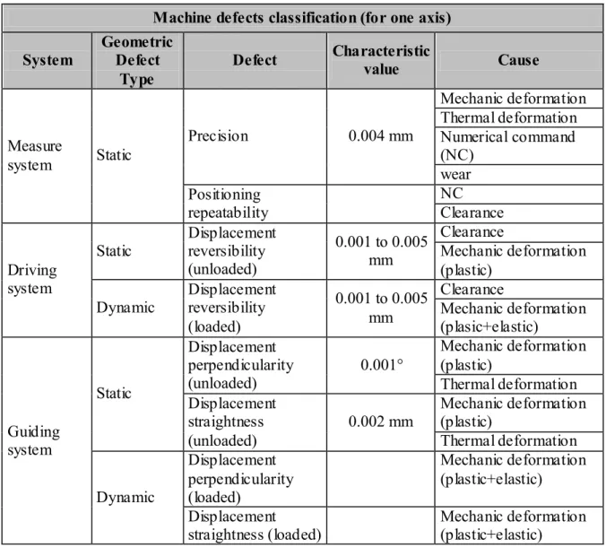
The machine used is a three axes NC vertical milling machine. The technical specifications are available in the annex. The different type of defect that characterize our machine capability are first defined (Table 2, Table 3, Table 4), then we will focus on the geometric defects and define the values of the machine’s defects from experiences. To finish, we will approximate those defects.
Table 2: Geo metric defects in a nu merically controlled mach ine (for one axis) Table 3 : Defects of the tool, fixtures and work piece
Table 4 : Defects of the surface plate
We focus on the following static geometrical defects:
- Displacement perpendicularity (also called axis orientation),
- Displacement straightness (it must be noticed that this type of defect is composed of 5 degrees of freedom: 2 translations called straightness and 3 rotations called rotations),
- Work piece position (because of set-up errors or defective geometry of the work piece before machining).
Table 5 gives the influence of work cell defect (addition of machine, work piece, and fixture defects) on the machined work piece accuracy (which work cell defect causes what type of work piece geometric error).
Table 5 : Influence of work cell defects on work piece geo metric accuracy.
In order to predict the work piece defects with the best accuracy, we decide to base them on the real machine defects measurements:
- The out of parallelism and lack of perpendicularity for each axis. - The unevenness of the table.
- The straightness of the axis.
- The rotation error of the axis (Yaw, Pitch, Roll). - Axial position error.
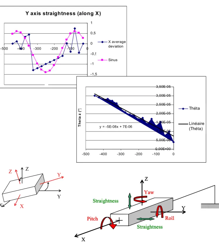
From the kinematic errors measurements, a mathematical function gives us an estimation of the error all alo ng the displacement range. Graphs (Figure 7) give the axis defect (orthogonal translation or rotation) for each
point of the axis. In order to simplify the problem, we will approximate those graphs with mathematical functions such as Sine or linear interpolation.
Figure 7: Identification of X axis defect
The graphs of the straightness defect Y following the X displacement can be approximated with a Sine function which represents the waviness of the slide:
Y = sin (0.8 * X)
The graphs of the pitch rotation x defect following the X displacement can be approximated with a linear regression which gives a linear function which represents a small torsion of the slide.
x = -8 * 10 -8 X
The static error measures are based on a table that gives the out of parallelism and the lack of perpendicularity of the different axes with respect to the plane surface. From those results, the exact orientation error measurement (Table 6) is deduced.
Table 6 : Defects approximations mathematic functions
4.3. Designing the virtual machine and assigning kinematics
The design of the virtual machine is done with the help of DELMIA software (robotic module). Here all the PARTS (components of the machine) are created in the CAD module, and by jointing them we obtain a complete WORKCELL (name given by the software for the machine and the work piece fixed on the table). Modelling a machine consists in building Devices ( PARTS) and then jointing them into a Machine following the kinematic structure. Building a Device consists in positioning the different Parts and then jointing them by a kinematic joint. Each joint is between two Parts, one will be the parent Part, and the other will be the Part that will move. The work cell is the assembly of the Machine, the fixtures, the tool and the work piece.
In order to analyze the effects of the work cell (the whole machine) defects on the work piece, we decide to first study the effect of each type of joint defect, and then compare the work piece defects obtained with a complete work cell. We design five work cells, each one composed of the same machine, tool, fixtures and work piece but with five different types of defects: orientation, straightness, rotation, part position and the total (table 7).
Since we do not have measurements for the work piece positioning error, we assume an orientation error of 0.02/300mm for each work piece axis. This gives an orientation error (rotation) of 0.00382° on each axis.
4.4. Performing the simulation with and without including machine accuracy and set-up defects.
The motion simulation used is based on a kinematic analysis of the machine models. In this approach, motions are planned to satisfy the positioning requirements in the device configuration space and/or work cell Cartesian space. Two kinds of simulations are undertaken, first ones by considering a perfect machine, the others ones taking into account of the geometrical defects. For the simulation, each device follows precisely the motion planning commands in time, regardless of the forces (machining, friction…) and torques that cause
the geometrical defect of the kinematic chain. It is close to the real behaviour of an actual NC machine tool for finished machining of classical mechanical parts.
Each of the simulations will machine the same designed work piece (they all have the same machining program). The final machined work pieces should all be different, four of them being the result of a particular type of work cell defect and a fifth being the result of all the work cell defects. Thus, we can compare the effects of each type of work cell defect on the work piece by analyzing each machined piece. Since the work cell measured defects are too low to have a visible effect on the work piece, we have decided to increase them (their magnitude) by 100.
Table 7 : Defects included in the machine fo r simu lation
5. Analysis results and observation
After simulation of the machining process (done in the Work cell space) we transfer the machined piece (the work piece) into the CAD space (CAD main menu): the measurements are done with the Analysis main menu (figure 8). The technique used is based on Vertices location (a vertex is a point created by the intersection of several surfaces). It is important to note that every part created or imported into the CAD module is only defined by sets of points (which define surfaces); the vertices are those definition points. The analysis process is the same for each part.
Plane surfaces measurements
1. Create an ideal square plane which is orthogonal to the normal vector of the theoretical surface,
2. Identify the lowest vertex of the machined surface by slowly translating our square surface from the top to the bottom of the piece (provided that the square plane is coloured differently from the work piece, we get the lowest vertex when the square plane just disappears, hidden by the machined surface),
3. Move the square plane so that the lowest vertex is included in the surface, 4. Identify the highest vertex in the same way,
5. Measure the difference between the two square planes (which corresponds to the difference of altitude between the top and the bottom vertex of the machined surface).
Slots measurements
1. Measure the casing of each slot by creating an ideal square plane (6 for each slot) with the same method as the plane surfaces measurements.
2. Note the coordinates of 5 points along each slot.
3. Carry out a linear regression of those 5 points to get the average straight line representing the axis of the slot. We infer the direction vector of each slot’s axis and then calculate the angles between them and with the X and Y axis.
4. Calculate the middle point between the first and the fifth point measured along the slot. The straight -line passing through this point and parallel to the X (or Y) axis is considered to be the projection of the slot axis on the X (or Y) axis. It is from this line that we will calculate the positioning error of the slot.
Since the axes of the cylinders are not defined by vertices, it is impossible to get any information on them. Therefore, we will create circular polygons that will close the cylinders and work with the centres of those polygons.
- For each cylinder, we draw two circular polygons that close the cylinders. Those polygons are built by clicking on the vertices that define the cylinders. Hence, they are the approximations of discs that have the same diameter as the cylinders and their respective centres are the same as those of the extremity circles of the cylinders,
- Note the centre point coordinates of each polygon of each cylinder,
- Infer the direction vector of each cylinder axis and then calculate the angles between them and with the Z axis,
- Calculate the middle point between the first and the second point measured by cylinder. The straight line passing through this point and parallel to the Z axis is considered to be the projection of the cylinder axis on the Z axis. It is from this line that we will calculate the positioning error of the cylinder,
- Results analysis.
After getting the errors measurements of each face analysed, all those measurements are synthesized to get the values of the work piece defects according to the work cell defects. Table 8 gives the final results and allows the comparisons.
Table 8 : Work p iece geo metric erro r values in function of work cell defect 5.1. First analysis: part geometric errors (table 8)
Observations
- Face B unevenness is lower than face A unevenness because the area of A is larger (figure 6).
- Side thickness of the slots casings are almost equal to B unevenness. It is more significant for slot YS (figure 6) because it corresponds to a parallel machined surface,
- Casing thickness of both slots are equivalent. It means that the X and Y machine axes have the same defects (it is not true for the “overall “ work cell defects)
- Except for the straightness defect, the side thickness of the slots casing is almost equal to the slots parallelism errors. It means that the slots form error is negligible compared to the parallelism error. There is no form error in this case but only parallelism error.
- Parallelism error along Z for d axis is always higher than for D axis,
- Since hole D parallelism error along Z axis is low, the d/D parallelism error is higher or equal to the d/Z parallelism error (except for piece_pos workcell defect),
- Even if slots parallelism errors with respect to X and Y axes are high, the perpendicularity error between them is low (except for Rotation where the slots perpendicularity is an addition of the two parallelism errors), - Holes d and D locating errors are equivalent,
- Slots XS and YS location are completely different for the same work cell defect.
5.2. Second analysis: Defects versus defects
Table 9 gives the classification of the work cell defects as a function of how high its influence on the piece error is:
- Classification for A unevenness and slot bottom casing are the same because they are two parallel machined surfaces,
- Classification for B unevenness and slot bottom casing are the same because they are two parallel machined surfaces,
- A piece position error seems to be the first cause of most form and orientation errors less for location errors. However, we must note that the magnitude of the piece position defect is ten times higher than the other work cell defects,
- A rotation defect is the first cause of the location errors and the second cause for most of the form and orientation errors,
- Straightness defects are less responsible for the form errors of Z orthogonal surfaces. It is also less responsible for the d and D axes orientation errors,
- Orientation defects are less responsible for the form errors of X and Y orthogonal surfaces. It is also less responsible for the XS and YS orientation errors,
- Provided that piece positioning defect is the most influencing work cell defect for most of piece errors, we can say that it is the defect that leads to the worst final work piece. Nevertheless, this conclusion depends on which piece error is really unwanted by the user; if it is the location error, then the defect that leads to the worst final work piece is the rotation.
Table 9 : Work cell defects classification
5.3. Third analysis: Defects versus total
Table 10 presents the work piece error results of the overall work cell defect and compares them with the results of the work cell defect which leads to the closest error:
- The errors of the “total” work cell defect are neither equal to the highest error of the other work pieces nor an exact addition of all the other work piece errors. Hence, some geometric errors (from the different work cell defects) could cancel each other. Since the “total” work piece is machined by a machine which has a combination of all the work cell defects, it should be a combination of all the geometric errors.
- Strangely enough, certain “total” piece errors are higher than the addition of all the geometric errors (D location for example).
- It seems that for the piece location errors, the closest defect is the rotation which is also the most influent defect. However, the piece location errors of the “total” work cell defect are definitely higher.
Table 10 : Work cell co mplete error co mpared to the closest work cell error value
6. Conclusions
It is critical to analyze the results of the different work piece errors in order to highlight the redundancy of some errors (side casing error and parallelism error for example). It also helps to notice which piece geometry is more damaged by work cell defects or what is the behaviour of the different piece geometries (are they all damaged together, by two…?).
It is important to analyze and compare the consequences of each work cell defect on the work piece in order to know which work cell defect leads to the worst part defect. It could help the user to focus on the work cell
defect that causes the most unwanted part error. The defined work piece is a test work piece which allows to see and highlight basic geometric errors and to make good comparisons between the work cell defects.
It is interesting to compare the consequences of a complete work cell defect to the consequences of each single particular defect in order to know if it is a simple combination of piece errors or an obvious relation between work cell defects and part errors. Our results show us that the piece error of the complete work cell defect is not equal to the highest part error, some defects counteracting other ones.
The combination of the work cell defects leads to two possibilities: - They cancel each other and thus the piece error becomes smaller, - They enhance each other and thus the piece error becomes larger.
The machining simulation with a machine that has all the defects allows predicting the work piece errors due to machine geometric limitations. Then, the user can anticipate those errors and manage to reduce the influence of the work cell defects. For example, it is possible to design an NC program which creates a work piece with the opposite direction errors if they are important and reproducible; the combination with a limited machine could result in a perfect work piece.
The inclusion of machine accuracy in a virtual model of an NC machine allows us to present many advantages:
- The first is the ability of virtual machining to give a prediction of the machined work piece at a low cost. Actually, money is saved because material is not used and time is saved on the real machine. This way -we can virtually machine a lot of test work pieces to validate a process or a machine operation.
- Secondly, compared to a perfect virtual machine, the virtual realistic machine here developed gives a better representation of the real machine. It means that the machined work piece will be closer to the work pieces machined with a real machine.
- Third, it allows to study the consequences of each machine defect on the work piece geometric errors. As a result, it could appear that certain kinds of machine defects have no influence on the work piece and other machine defects can damage dangerously the work piece.
- Finally, since we can have a prediction of the machined work piece, we can reduce its geometric errors by designing an NC program that takes into account those errors (optimized conditions).
A modified NC program with a defective machine could produce a perfect work piece, if the errors are repeatable.
Obviously, the inclusion of machine accuracy is not realistic if the used software is not accurate enough. The results show that the software can predict machine defects influence on work piece since they are higher than:
- Standard Conditions: 0.002 mm - Optimized Conditions: 0.0002 mm References
Sohlenius S. , 1992, “Concurrent engineering”, Annals of the CIRP - 41/2, p645-655
Altintas Y., Brecher C., Weck M., Witt C., 2005, “Virtual Machine Tool”, Annals of the CIRP, 54/2, pp. 651-674
Bianchi G., F. Paolucci, F., Van den Braembussche P., Jovane F., 1996, Toward virtual engineering in machine-tool design, Annals of the CIRP, 45/1, pp. 381 -386
RogstrandV., KjellbergT. , 2009, “The representation of manufacturing requirements in model-driven parts manufacturing” International Journal of Computer Integrated Manufacturing, Volume 22, Issue 11 , pages 1054 - 1064
SamantaB., 2009, Surface roughness prediction in machining using soft computing , International Journal of Computer Integrated Manufacturing, Volume 22, Issue 3 , pages 257 - 266
Yang J.; HanS. ; Kan H. ; KimJ., 2006, Product data quality assurance for e-manufacturing in the
automotive industry, International Journal of Computer Integrated Manufacturing, Volume 19, Issue2, pages 136 – 147
Jun Y.; LiuJ. ; NingR. ; ZhangY., 2005, Assembly process modeling for virtual assembly process planning School of Mechanical and Vehicle Engineering, International Journal of Computer Integrated
Manufacturing, Volume 18, Issue 6 ,, pages 442 - 451
Martin P., D’Acunto A., 2003, “Design of a production system: an application of integration product-process”, Int. J. Computer Integrated Manufacturing, Vol.16, N° 7-8, pp 509-516
Martin P., Schneider F., Dantan J. Y., 2005, "Optimal adjustment of a machine tool for improving the geometrical quality of machined part", International Journal on Advanced Manufacturing, n°26, pp. 559-564
Reshetov D. N., Portman V. T., 1988, “Accuracy of machine tools”, ASME press, New York, ISBN 0-7918-0004-0
Weck M., 1984, Handbook of Machine Tools, Johh Wiley and Sons, New York
SME, 1976, “Tool and Manufacturing Engineers Handbook”, Society of Manufacturing Engineers, McGraw-Hill, New York, 1976
Bohez, E.L.J, 2002, Five-axis milling machine tool kinematic chain design and analysis, Journal of Machine tools and Manufacture, 42, pp.505-520.
Garro O., Martin P., 1993, “ Towards new architectures of Machine Tools”, Int. J. of Production Research, Vol. 31, n° 10, pp. 2403-2414
Koren, Y, Moriwaki, T, Van Brussel, H, 1999, “Reconfigurable Manufacturing Systems”, Annals of the CIRP, 48, 527-540
Bourdet P. , Clément A., 1988, “A study of optimal- criteria identification based on small displacement screw model”, Annals of the CIRP, vol. 37, pp. 503-506
Shabaka A.I.; Elmaraghy H.A. , 2007, Generation of machine configurations based on product features International Journal of Computer Integrated Manufacturing, Volume 20, Issue 4 , pages 355 – 369 D’Acunto A., Martin P., Aladad H., 2007, “Design of Reconfigurable Machine Tool: Structural Creating and
Kinematical Model” 40ème CIRP International Seminar on Manufacturing Systems, Liverpool, may 30 – june 1
Moon Y. and Kota S., 2002, “Generalized Kinematic Modeling of Reconfigurable Machine Tools”, ASME Transactions, Journal of Mechanical Design, V. 124.47, pp. 47-51
Tutenea-Fatan O., Feng H.Y.,2004, ”Configuration analysis of five-axis machine tools using a generic kinematic model”, International Journal of Machine Tools and Manufacture, 44, pp. 1235-1243, Kyoung-Gee Ahn, Byung-Kwon Min, Zbigniew J. Pasek, 2005, “Geometric error modelling and
compensation of a multi spindle reconfigurable machine tool”, 3rd International CIRP conference on Reconfigurable Manufacturing, may 19-12, University of Michigan, Ann Arbor, MI, USA
Ahn K. G., Cho D.W., 1999, “Proposition for a volumetric error model considering backlash in Machine Tools”, Int. J. of Advanced Manufacturing technology, Vol. 15, pp.554-561
Eman K. F., Wu B.T., 1987, “A generalized geometric error model for multi-axis machines”, Annals of the CIRP, 36/1, pp. 253-256
Chen F.C., 2000, “On the structural configuration synthesis and geometry of machine centres”. Proceedings of Instrumentation and Mechanics Engineers, N°. 215, p.641-652
Yao Y., Zhao H., Li J. and Yuan Z., 2006, “Modeling of virtual workpiece with machining errors representation in turning”, Journal of Materials Processing Technology, N° 172, pp. 437–444,
Chaiprapat S. and Rujikietgumjorn S., 2008, “Modeling of positional variability of a fixtured workpiece due to locating errors” Int. J. Advanced Manufacturing Technology , N° 36, pp.724–731
Yeh J.H., and Liou F. W., 1999, Contact condition modelling for machining fixture setup processes, International Journal of Machine Tools and Manufacture , N°39, pp. 787–803
Yeh J.H., and Liou F. W. ,2000, Clamping Fault Detection in a Fixturing System, Journal of Manufacturing Processes Vol. 2/No. 3
Anotaipaiboon S. Makhanov and. Bohez E.L.J., 2006, “Optimal setup for five-axis machining”, International Journal of Machine Tools and Manufacture, N° 46, pp. 964–977
7. Annex: Machine description
The machine that we will use is a three axes NC vertical milling machine SOMAB. It the following characteristics:
Structure
Support in granite Totally covered Spindle cone ISO 40. External lubrification.
Slide bar in solid treated steel.
Sliding assisted by some turcite sticked on all the slide ways.
Command achieved by ball screw and controlled by embedded coder.
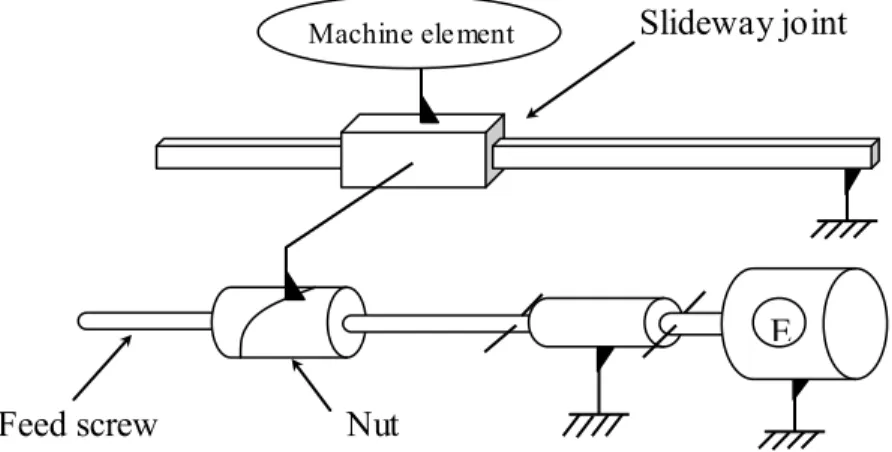
Greasing achieved by an automatic station. Kinematic schema
Each axis is composed of a set of 3 systems:
Z Y X Support Bench Square Pillar
- The measure system.
- The driving system (brushless motor and driving feed screw with nut). - The guiding system (slideway joint).
E
Machine element
Feed screw Nut
Slideway joint
Figure 2 : Geo metrical defin ition of mechanis m
C DC F
Nominal Geometry Small deviations
Dimensioning Tolerancing
Relation between parts Generation of faces Designed Solutions Manufacturing Processes Functionnal requirements DESIGNER MANUFACTURER METROLOGIST Conceptual Structural Parametric Real G e o m e tr ic a l d e fi n it io n o f m e c h a n is m P ro d u c t d e s ig n MODEL Generation of faces
Relation between parts
a : Arborescence structure of the manufacturing set-up process plan
b: contact schema: point concept
Figure 3 : Geo metrical defects due to set-ups PS21 PS31 Set-up 1 Set-up 2 Set-up 3 Part Base Reference Set-up 1 Reference Set-up 2 Reference Set-up 3 Reference PS22 PS21 PS31 Set-up 1 Set-up 2 Set-up 3 Part Base Reference Set-up 1 Reference Set-up 2 Reference Set-up 3 Reference PS22 PS12 PS11 PS13 PS23 PS12 PS11 PS13 Part 1 Part-holder Part 2 Part 1
Small displacement matrix Small displacement screw
yaw: pitch: roll:
Figure 5 : Small displacement matrix
tz
ty
tx
Figure 6 : Test part A A 50 50 90 120 55 90 20 20 40 20 A-A 50 10 40 B YS XS A d D
Figure 7 : Identification of X axis defect X Y X Y Z Z Yaw Roll Pitch Straightness Straightness X Z Y
Fig. Slideway joint defects
Yaw Roll Pitch Straightness Straightness X Z Y Yaw Roll Pitch Straightness Straightness X Z Y
Fig. Slideway joint defects
Y axis straightness (along X)
-2 -1,5 -1 -0,5 0 0,5 1 -500 -400 -300 -200 -100 0 Y X X average deviation Sinus
Z a xis rota tion (around Z)
y = -5E-08x + 7E-06 0,00E+00 5,00E-06 1,00E-05 1,50E-05 2,00E-05 2,50E-05 3,00E-05 3,50E-05 -500 -400 -300 -200 -100 0 Z (m m ) T h e ta z ( °) Théta Linéaire (Théta)
Distance Measure Angle Measure
Figure 8 : Part measurements
Machined
Geometry Location Name Error to be measured
Surfacing Top surface A Unevenness Surfacing Side surface B Unevenness
Slotting Along X axis XS Form error (casing) Parallelism along X Locating error Slotting Along Y axis YS Form error (casing)
Parallelism along Y
Perpendicularity with respect to XS Locating error
Drilling Along Z axis d Parallelism along Z Locating defect Drilling Along Z axis D Parallelism along Z
Parallelism with respect to d axis Locating error
Machine defects classification (for one axis) System Geometric Defect
Type
Defect Characteristic value Cause
Measure system Static Precision 0.004 mm Mechanic deformation Thermal deformation Numerical command (NC) wear Positioning repeatability NC Clearance Driving system
Static Displacement reversibility (unloaded) 0.001 to 0.005 mm Clearance Mechanic deformation (plastic)
Dynamic Displacement reversibility (loaded) 0.001 to 0.005 mm Clearance Mechanic deformation (plasic+elastic) Guiding system Static Displacement perpendicularity (unloaded) 0.001° Mechanic deformation (plastic) Thermal deformation Displacement straightness (unloaded)
0.002 mm Mechanic deformation (plastic) Thermal deformation Dynamic Displacement perpendicularity (loaded) Mechanic deformation (plastic+elastic) Displacement
straightness (loaded) Mechanic deformation (plastic+elastic)
Defect type Defect Characteristic value
Deformation Elastic deformation 0.02 mm
Thermal dilatation
Geometric - Static Orientation 0.02 °
Positioning 0.2 to 0.01 mm
Table 3: Defects of the tool, fixtures and work piece
Defect type Defect Characteristic
value
Geometric Unevenness 0.04/1000 mm
Dimension Position Shape Roughness Machine elements Measure system Driving system Guiding system Fixture & work piece
Fixture & work piece
Static defects (axis orientation) Axis Angle with respect to Error (in °)
X X 0 Y 0.955 Z 0.382 Y X 0.955 Y 0 Z 0.382 Z X 2.86 Y 2.86 Z 0 Kinematics defects
Axis Defect respect to With Math function
X
Straightness Y Z y = sin(0.8*x) z = sin(0.8*x) Rotation Rx θx = -5.5*10-05*x Ry θy = -3*10-05*x Rz θz = -5.5*10-05*x Y Straightness X x = sin(1.03*y) Z z = 1.5*sin(0.6*y) Rotation Rx θx = -8*10-05*y Ry θy = -5.5*10-05*y Rz θz = -5.5*10-05*y Z Straightness X X = sin(0.8*z) Y y = sin(0.8*z) Rotation Rx θx = -5.5*10-05*z Ry θy = -5.5*10-05*z Rz θz = -5*10-05*z
Workcell’s
Name Defect included in the machine
Orientation Machine axes orientation (3 angles).
Straightness Machine axes straightness (2 translations /axis).
Rotation 3 rotations (Yaw, Pitch, Roll) per axis. Part_position Piece orientation (3 angles).
TOTAL All the previous defects. Table 7: Defects included in the machine for simulation
Workcell defects
Orientation Straightness Rotation Piece_pos TOTAL
P ie ce e rr or s (m m ) F or m Unevenness A 6,23 3,19 13,42 18,15 18,61 Unevenness B 1,33 1,62 4,14 14,70 13,26 X slot casing Sides 1,22 1,95 2,16 12,58 5,59 Bottom 3,21 1,97 7,32 14,93 17,31 Y slot casing Sides 1,33 1,60 2,55 13,83 10,53 Bottom 3,50 1,33 7,36 13,80 2,76 O ri en ta ti on d / Z axis parallelism 1,03 0,29 2,72 4,72 1,10 D / Z axis parallelism 0,01 0,005 1,68 4,72 3,07 D / d axes parallelism 1,04 0,28 2,99 6,64 3,87 XS / X axis parallelism 1,33 4,40 1,94 12,46 6,29 YS / Y axis parallelism 1,33 2,72 2,43 13,35 12,13 XS / YS axis perpendicularity 0,0004 1,68 4,37 0,88 5,83 P os it ion d axis locating 11,54 0,64 22,17 6,90 47,30 D axis locating 12,79 0,33 17,59 5,08 42,07 XS axis locating 1,69 2,32 19,39 2,81 37,85 YS axis locating 10,74 0,89 12,69 3,12 25,63
Piece error type Classification
F
or
m
Unevenness A Straight. Orient. Rot. Piece_ pos
Unevenness B Orient. Straight. Rot. Piece_ pos
Slots sides casing Orient. Straight. Rot. Piece_ pos
Slots bottom casing Straight. Orient. Rot. Piece_ pos
O ri ent at i on
D & d parallelism (/Z) Straight. Orient. Rot. Piece_ pos
D / d parallelism Straight. Orient. Rot. Piece_ pos
XS & YS parallelism Orient. Rot. Straight. Piece_ pos Slot perpendicularity Orient. Piece_ pos Straight. Rot.
L
oc
at
ion d locating D locating Straight. Straight. Piece_ pos Piece_ pos Orient. Orient. Rot. Rot.
XS locating Orient. Straight. Piece_ pos Rot.
YS locating Straight. Piece_pos Orient. Rot.
Table 9 : Work cell defects classification
Piece error type TOTAL Value Closest work cell defect Value work cell Highest defect Value F or m
Unevenness A 18.61 Piece_pos 18.15 Piece_pos 18.15
Unevenness B 13.26 Piece_pos 14.70 Piece_pos 14.70
XS sides casing 5.59 Rotation 2.16 Piece_pos 5.59
XS bottom casing 17.31 Piece_pos 14.93 Piece_pos 14.93 YS sides casing 10.53 Piece_pos 13.83 Piece_pos 13.83 YS bottom casing 2.76 Orientation 3.50 Piece_pos 13.8
O
ri
ent
at
ion
d/Z parallelism 1.10 Orientation 1.03 Piece_pos 4.72
D/Z parallelism 3.07 Rotation 1.68 Piece_pos 4.72
D / d parallelism 3.87 Rotation 2.99 Piece_pos 6.64
XS/X parallelism 6.29 Straightness 4.40 Piece_pos 12.46 YS/Y parallelism 12.13 Piece_pos 13.35 Piece_pos 13.35
XS/YS perpend. 5.83 Rotation 4.37 Rotation 4.37
L
oc
at
ion D locating D locating 47.30 42.07 Rotation Rotation 22.17 17.59 Rotation Rotation 22.17 17.59
XS locating 37.85 Rotation 19.39 Rotation 19.39
YS locating 25.63 Rotation 12.69 Rotation 12.69