Science Arts & Métiers (SAM)
is an open access repository that collects the work of Arts et Métiers Institute of
Technology researchers and makes it freely available over the web where possible.
This is an author-deposited version published in: https://sam.ensam.eu
Handle ID: .http://hdl.handle.net/10985/6274
To cite this version :
Etienne PRULIERE, Francisco CHINESTA, Amine AMMAR - On the deterministic solution of multidimensional parametric models using the Proper Generalized Decomposition - 2010
On the deterministic solution of
multidimensional parametric
models using the Proper
Generalized Decomposition
E. Pruliere
1, F. Chinesta
2,3, A. Ammar
41Arts et M´etiers ParisTech
Esplanade des Arts et M´etiers, 33405 Talence cedex, France 2GeM: UMR CNRS – Centrale Nantes
1 rue de la No¨e, BP 92101, F-44321 Nantes cedex 3, France
3EADS Corporate Foundation Internantional Chair – GeM – Centrale Nantes 4Laboratoire de Rh´eologie: UMR CNRS – UJF – INPG
1301 rue de la piscine, BP 53, F-38041 Grenoble, France
Abstract: This paper focuses on the efficient solution of models defined in
high dimensional spaces. Those models involve numerous numerical challenges because of their associated curse of dimensionality. It is well known that in mesh-based discrete models the complexity (degrees of freedom) scales exponentially with the dimension of the space. Many models encountered in computational science and engineering involve numerous dimensions called configurational co-ordinates. Some examples are the models encountered in biology making use of the chemical master equation, quantum chemistry involving the solution of the Schr¨odinger or Dirac equations, kinetic theory descriptions of complex sys-tems based on the solution of the so-called Fokker-Planck equation, stochastic models in which the random variables are included as new coordinates, financial mathematics, ... This paper revisits the curse of dimensionality and proposes an efficient strategy for circumventing such challenging issue. This strategy, based on the use of a Proper Generalized Decomposition, is specially well suited to treat the multidimensional parametric equations.
Keywords: Multidimensional models; Curse of dimensionality; Parametric
1
Introduction: revisiting the Proper
General-ized Decomposition
The efficient solution of complex models involving an impressive number of de-grees of freedom could be addressed by performing high performance computing (in general making use of parallel computing platforms) or by speeding up the calculation by using preconditioning, domain decomposition, ...
In the case of transient models the use of model reduction can alleviate significantly the solution procedure. The main ingredient of model reduction techniques based on the use of proper orthogonal decompositions -POD- consists of extracting a reduced number of functions able to represent the whole time evolution of the solution, that could be then used to make-up a reduced model. This extraction can be performed by invoking the POD. The reduced model can be then used for solving a similar model, i.e. a model slightly different to the one that served to extract the reduced approximation basis, or for solving the original model in a time interval larger than the one that served for constructing the reduced basis. The main issue in this procedure consists in the evaluation of the reduced basis quality when it applies in conditions beyond its natural interval of applicability. In order to ensure the solution accuracy one should proceed to enrich the reduced approximation basis, and the definition of optimal, or at least efficient, enrichment procedures is a difficult task that remains at present an open issue.
Such model reduction strategies were successfully applied, in some of our for-mer works, to solve kinetic theory models [5] [23] allowing impressive computing-time savings. The main conclusion of our former works was the fact that an accurate description of a complex system evolution can, in general, be per-formed from the linear combination of a reduced number of space functions (defined in the whole space domain). The coefficients of that linear combina-tion evolve in time. Thus, during the resolucombina-tion of the evolucombina-tion problem, an efficient algorithm has to compute the approximation coefficients and to enrich the approximation basis at the same time. An important drawback of one such approach is the fact that the approximation functions are defined in the space domain. Until now, the simplest form to represent one such function is to give its values in some points of the domain of interest, and to define its values in any other point by interpolation. However, sometimes models are defined in multidimensional spaces and in this case the possibility of describing functions from their values at the nodes of a mesh (or a grid in the domain of interest) can become prohibitory.
Many models encountered in computational science and engineering involve numerous dimensions called configurational coordinates. Some examples are the models encountered in biology making use of the chemical master equation, quantum chemistry involving the solution of the Schr¨odinger or Dirac equations, kinetic theory descriptions of complex materials and systems based on the so-lution of the so-called Fokker-Planck equation, stochastic models in which the random variables are included as new coordinates, financial mathematics
model-ing credit risk in credit markets (multi-dimensional Black and Scholes equation), ... The numerical solution of those models introduces some specific challenges related to the impressive number of degrees of freedom required because of the highly dimensional spaces in which those models are defined. Despite the fact that spectacular progresses have been accomplished in the context of compu-tational mechanics in the last decades, the treatment of those models, as we describe in the present work, requires further developments.
The brut force approach cannot be considered as a possibility for treating this kind of models. Thus, in the context of quantum chemistry, the Nobel Prize laureate R.B. Laughlin, affirmed that no computer existing, or that will ever exist, can break the barriers found in the solution of the Schr¨odinger equation in multi-particle systems, because of the multidimensionality of this equation [15].
We can understand the catastrophe of dimension by assuming a model de-fined in a hyper-cube in a space of dimension D, Ω =]− L, L[D. In fact, if we
define a grid to discretize the model, as it is usually performed in the vast ma-jority of numerical methods (finite differences, finite elements, finite volumes, spectral methods, etc.), consisting of N nodes on each direction, the total num-ber of nodes will be ND. If we assume that for example N ≈ 10 (an extremely coarse description) and D≈ 80 (much lower than the usual dimensions required in quantum or statistical mechanics), the number of nodes involved in the dis-crete model reaches the astronomical value of 1080that represents the presumed
number of elementary particles in the universe! Thus, progresses on this field need the proposal of new ideas and methods in the context of computational physics.
A first solution is the use of sparse grids methods [8], however as argued in [1], this strategy fails when it applies for the solutions of models defined in spaces whose dimension are about 20.
Another possible alternative for circumventing, or at least alleviating the curse of dimensionality issue, consists of using separated representations within the context of the so-called Proper Generalized Decomposition. We proposed recently a technique able to construct, in a completely transparent way for the user, the separated representation of the unknown field involved in a par-tial differenpar-tial equation. This technique, originally described and applied to multi-bead-spring FENE models of polymeric systems in [3], was extended to transient models of such complex fluids in [4]. Other more complex models (in-volving different couplings and non-linearities) based on the reptation theory of polymeric liquids were analyzed in [17]. This technique was also applied in the fine description of the structure and mechanics of materials [11], including quantum chemistry [2], and in materials homogenization [12]. Some numerical results concerning this kind of approximation were addressed in [22] and [7].
Basically, the separated representation of a generic function u(x1,· · · , xD)
u(x1,· · · , xD)≈ i=N∑
i=1
F1i(x1)× · · · × FDi(xD) (1)
This kind of representation is not new, it was widely employed in the last decades in the framework of quantum chemistry. In particular, the Hartree-Fock (that involves a single product of functions) and the post-Hartree-Hartree-Fock approaches (as the MCSCF that involves a finite number of sums) are based on a separated representation of the wavefunction [10]. Moreover, Pierre Ladeveze [14] proposed many years ago a space-time separated representation (that he called radial approximation) within the context of the incremental non-linear solver LATIN. This technique allowed impressive computing time savings in the simulation of usual 3D transient models because of its intrinsic non-incremental character.
Separated approximations are an appealing choice for addressing the solution of stochastic models [19]. Usually, stochastic equations are based on simple deterministic solvers in the context of Monte-Carlo methods [9] [20] or some equivalent methods [21] [6]. The main difficulty of this kind of methods is the need of a large amount of deterministic computations to approach the response of a given probability distribution. An alternative to these methods consists on the use of direct simulations describing explicitly the stochastic variables with a Galerkin approximation [13] [16]. Obviously, these strategies are restricted by the curse of dimensionality. The use of Proper Generalized Decomposition can extend the application field of deterministic solvers to models including many stochastic parameters, that will be introduced as new model coordinates. The interested reader can refer to the excellent review of A. Nouy [18].
In this present paper the PGD technique is revisited and then used to address some linear and non-linear parametric models.
2
Illustrating the solution of multidimensional
parametric models by using the PGD
In what follows we are illustrating the construction of the Proper General-ized Decomposition by considering a quite simple problem, the parametric heat transfer equation:
∂u
∂t − k∆u − f = 0 (2)
where (x, t, k)∈ Ω × I × ℑ and for the sake of simplicity the source term is as-sumed constant, i.e.f = cte. Because the conductivity is considered unknown, it is assumed as a new coordinate defined in the intervalℑ. Thus, instead of solving the thermal model for different values of the conductivity parameter we prefer introducing it as a new coordinate. The price to be paid is the in-crease of the model dimensionality; however, as the complexity of PGD scales linearly with the space dimension the consideration of the conductivity as a new coordinate allows faster and cheaper solutions.
We look to the solution of Eq. (2) as:
u (x, t, k)≈
i=N∑ i=1
Xi(x)· Ti(t)· Ki(k) (3)
For the following equation the approximation at iteration n is supposed known:
un(x, t, k) =
i=n
∑
i=1
Xi(x)· Ti(t)· Ki(k) (4)
Thus, we look for the next functional product Xn+1(x)· Tn+1(t)· Kn+1(k)
that for alleviating the notation will be denoted by R (x)· S (t) · W (k). Before solving the resulting non linear model related to the calculation of these three functions a model linearization is required. The simplest choice consists in using an alternating directions fixed point algorithm. It proceeds by assuming
S (t) and W (k) given at the previous iteration of the non-linear solver and
then computing R (x). From the just updated R (x) and W (k) we can update
S (t), and finally from the just computed R (x) and S (t) we compute W (k).
The procedure continues until reaching convergence. The converged functions
R (x), S (t) and W (k) allow defining the searched functions: Xn+1(x) = R (x),
Tn+1(t) = S (t) and Kn+1(k) = W (k). These three steps can be detailed as
follows.
Computing R (x) from S (t) and W (k):
We consider the global weak form of Eq. (2): ∫ Ω×I×ℑ u∗ ( ∂u ∂t − k∆u − f ) dx dt dk = 0 (5)
where the trial and test functions write respectively:
u (x, t, k) = i=n ∑ i=1 Xi(x)· Ti(t)· Ki(k) + R (x)· S (t) · W (k) (6) and u∗(x, t, k) = R∗(x)· S (t) · W (k) (7) Introducing (6) and (7) into (5) it results
∫ Ω×I×ℑ R∗· S · W ·(R·∂S ∂t · W − k · ∆R · S · W ) dx dt dk = =− ∫ Ω×I×ℑ R∗· S · W ·Rn dx dt dk (8)
whereRn defines the residual at iteration n that writes:
Rn= i=n ∑ i=1 Xi· ∂Ti ∂t · Ki− i=n ∑ i=1 k· ∆Xi· Ti· Ki− f (9)
Now, knowing all the functions involving time and parametric coordinate, we can integrate terms of Eq. (8) in their respective domains I× ℑ. By integrating over I× ℑ and taking into account the notations:
w1= ∫ ℑ W2dk s1= ∫ I S2dt r1= ∫ Ω R2dx w2= ∫ ℑ kW2dk s2= ∫ I S·dSdtdt r2= ∫ Ω R· ∆R dx w3= ∫ ℑ W dk s3= ∫ I S dt r3= ∫ Ω R dx wi 4= ∫ ℑ W · Ki dk si4= ∫ I S·dTi dtdt r i 4= ∫ Ω R· ∆Xi dx w5i = ∫ ℑ kW · Ki dk si5= ∫ I S· Ti dt ri5= ∫ Ω R· Xi dx (10)
the Eq. (8) reduces to: ∫ Ω R∗· (w1· s2· R − w2· s1· ∆R) dx = =−∫ Ω R∗· (i=n∑ i=1 wi 4· si4· Xi− i=n∑ i=1 wi 5· si5· ∆Xi− w3· s3· f ) dx (11)
Eq. (11) defines an elliptic steady state boundary value problem that can be solved by using any discretization technique operating on the model weak form (finite elements, finite volumes . . . ). Another possibility consists in coming back to the strong form of Eq. (11):
w1· s2· R − w2· s1· ∆R = =− (i=n ∑ i=1 wi4· si4· Xi− i=n ∑ i=1 w5i· si5· ∆Xi− w3· s3· f ) (12)
that could be solved by using any collocation technique (finite differences, SPH, etc).
Computing S (t) from R (x)and W (k):
In the present case the test function writes:
u∗(x, t, k) = S∗(t)· R (x) · W (k) (13) Now, the weak form writes:
∫ Ω×I×ℑ S∗· R · W ·(R·∂S∂t · W − k · ∆R · S · W) dx dt dk = =− ∫ Ω×I×ℑ S∗· R · W ·Rn dx dt dk (14)
After integration in the space Ω× ℑ and taking into account the notation (10) we obtain: ∫ I S∗·(w1· r1·dSdt − w2· r2· S ) dt = =−∫ I S∗· (i=n∑ i=1 wi4· ri5·dTdti− i=n∑ i=1 w5i· ri4· Ti− w3· r3· f ) dt (15)
Eq. (15) represents the weak form of the ODE defining the time evolution of the field S that can be solved by using any stabilized discretization technique (SU, Discontinuous Galerkin, . . . ). The strong form of Eq. (15) is:
w1· r1· dS dt − w2· r2· S = =− (i=n ∑ i=1 w4i· ri5·dTi dt − i=n ∑ i=1 w5i· r4i· Ti− w3· r3· f ) (16)
This equation can be solved by using backward finite differences, or higher order Runge-Kutta schemes, among many other possibilities.
Computing W (k) from R (x)and S (t):
In the present case the test function writes:
u∗(x, t, k) = W∗(k)· R (x) · S (t) (17) Now, the weak form reads
∫ Ω×I×ℑ W∗· R · S·(R·∂S∂t · W − k · ∆R · S · W) dx dt dk = =− ∫ Ω×I×ℑ W∗· R · S·Rn dx dt dk (18)
that integrating in the space Ω× I and taking into account the notation (10) results: ∫ ℑ W∗· (r1· s2· W − r2· s1· W ) dk = =−∫ ℑ W∗· (i=n∑ i=1 ri5· si4· Ki− i=n∑ i=1 ri4· si5· Ki− r3· s3· f ) dk (19)
Eq. (19) does not involve any differential operator. The strong form of Eq. (19) is: (r1· s2− r2· s1)· W = − (i=n ∑ i=1 ( ri5· si4− r4i· si5 ) · Ki− r3· s3· f ) (20)
that represents an algebraic equation. Thus, the introduction of parameters as additional model coordinates has not a noticeable effect in the computational cost, because the original equation does not contain derivatives with respect to those parameters.
There are other minimization strategies more robust and exhibiting faster convergence for building-up the PGD, that we introduce in the next section in which the PGD constructor is presented in a matrix form.
3
A general formalism for the PGD
3.1
Separated representations
In what follows we are summarizing the main ideas that the Proper General-ized Decomposition (PGD) technique involves in a general formalism. For that purpose we suppose the following discrete form:
U∗TAU = U∗TB (21)
U and U∗T are the discrete description of both the trial and the test fields
respectively. We assume that the problem is defined in a space of dimension D and can be written in a separated form:
A = nA ∑ i=1 Ai1⊗ Ai2⊗ · · · ⊗ AiD B = nB ∑ i=1 Bi1⊗ Bi2⊗ · · · ⊗ BiD U = n ∑ i=1 ui1⊗ u i 2⊗ · · · ⊗ u i D (22)
The separated representation ofA and B comes directly from the differential operators involved in the PDE weak form.
3.2
Building-up the separated representation
At iteration n, vectors uij, ∀i ≤ n and ∀j ≤ D are assumed to be known. Now we are looking for an enrichment:
U =
n
∑
i=1
ui1⊗ · · · ⊗ uiD+ R1⊗ · · · ⊗ RD (23)
where Ri, i = 1,· · · , D, are the unknown enrichment vectors. We assume the
following form of the test field:
U∗= R∗
1⊗ R2⊗ · · · ⊗ RD+· · · + R1⊗ · · · ⊗ RD−1⊗ R∗D (24)
Introducing the enriched approximation into the weak form, the following discrete form results:
nA ∑ i=1 n ∑ j=1 (R∗1)TAi1u j 1× · · · × (RD)TAiDu j D+· · · + + nA ∑ i=1 n ∑ j=1 (R1)TAi1u j 1× · · · × (R∗D) TAi Du j D +
+ nA ∑ i=1 (R∗1)TAi1R1× · · · × (RD)TAiDRD+· · · + + nA ∑ i=1 (R1)TAi1R1× · · · × (R∗D) TAi DRD = = nB ∑ i=1 ( (R∗1)TBi1× · · · × (RD)TBiD +· · · + (R1)TBi1× · · · × (R∗D) TBi D ) (25) For the sake of clarity we introduce the following notation:
nC ∑ i=1 Ci1⊗ · · · ⊗ CiD= nB ∑ i=1 Bi1⊗ · · · ⊗ BiD− nA ∑ i=1 n ∑ j=1 Ai1uj1⊗ · · · ⊗ AiDujD (26) where nC = nB + nA× n. This sum contains all the known fields. Thus Eq.
(25) can be written as:
+ nA ∑ i=1 (R∗1)TAi1R1× · · · × (RD)TAiDRD+· · · + + nA ∑ i=1 (R1)TAi1R1× · · · × (R∗D)TAiDRD = = nC ∑ i=1 ( (R∗1)TCi1× · · · × (RD)TCiD +· · · + (R1)TCi1× · · · × (R∗D)TCiD ) (27) This problem is strongly non linear. To solve it, an alternated directions scheme is applied. The idea consists to start with the trial vectors R(0)i , i = 1,· · · , D or to assume that these vector are known at iteration p, R(p)i , i = 1,· · · , D, and to update them gradually using an appropriate strategy. We can either: • Update vectors R(p+1) i , ∀i, from R (p) 1 ,· · · , R (p) i−1, R (p) i+1,· · · , R (p) D . or: • Update vectors R(p+1) i , ∀i, from R (p+1) 1 ,· · · , R (p+1) i−1 , R (p) i+1,· · · , R (p) D .
The last strategy converges faster but the advantage of the first one is the possibility of updating each vector simultaneously making use of a parallel com-puting platform. The fixed point of this iteration algorithm allows defining the enrichment vectors un+1i = Ri, i = 1,· · · , D.
When we look for vector Rk assuming that all the others Ri, i ̸= k are
known, the test field reduces to:
U∗T = R
The resulting discrete weak form writes: nA ∑ i=1 ( RT1Ai1R1× · · · × R∗Tk A i kRk× · · · × RTDA i DRD ) = = nC ∑ i=1 RT1Ci1× · · · × R∗Tk Cik× · · · × RTDCiD (29) By applying the arbitrariness of R∗Kthe following linear system can be easily obtained: ( nA ∑ i=1 ( D ∏ j=1,j̸=k RT jAijRj ) Ai k ) Rk = nC ∑ i=1 ( D ∏ j=1,j̸=k RT jCij ) Ci k (30)
which can be easily solved.
3.3
Residual minimization
We have noticed that if instead of using the alternated directions iteration within the Galerkin framework for computing vectors Ri, we compute these vectors by
minimizing the residual:
Res = nA ∑ i=1 Ai1R1⊗ · · · ⊗ AiDRD− nC ∑ i=1 Ci1⊗ · · · ⊗ CiD (31) the convergence is significantly enhanced specifically for non symmetric opera-tors A.
We denote ⟨., .⟩ a scalar product and ∥.∥ its associated norm. Using this notation the residual norm writes:
∥Res∥2 = nA ∑ i=1 nA ∑ j=1 (⟨ Ai 1R1, A j 1R1 ⟩ × · · · ×⟨Ai DRD, A j DRD ⟩) − −2n∑A i=1 nC ∑ j=1 (⟨ Ai 1R1, C j 1 ⟩ × · · · ×⟨Ai DRD, C j D ⟩) + + nC ∑ i=1 nC ∑ j=1 (⟨ Ci 1, C j 1 ⟩ × · · · ×⟨Ci D, C j D ⟩) (32)
The minimization problem with respect to Rk reads:
∂
∂Rk ⟨Res, Res⟩ = 0
or: nA ∑ i=1 nA ∑ j=1 ⟨ Ai1R1, Aj1R1 ⟩ × · · · ×⟨Aik−1Rk−1, Ajk−1Rk−1 ⟩ × ×⟨Aik, AjkRk ⟩ ×⟨Aik+1Rk+1, A j k+1× Rk+1 ⟩ × · · · ×⟨AiDRD, A j DRD ⟩ − − nA ∑ i=1 nC ∑ j=1 ⟨ Ai1R1, Cj1 ⟩ × · · · ×⟨Aik−1Rk−1, Cjk−1 ⟩ × ×⟨Aik, Cjk ⟩ ×⟨Aik+1Rk+1, C j k+1 ⟩ × · · · ×⟨AiDRD, C j D ⟩ = 0 (34) The stopping criterion is defined from the residual norm:
nC ∑ i=1 Ci1⊗ · · · ⊗ CiD 2 < ϵ (35)
3.4
Remarks
It is important to notice that a general approximation in a domain consists in the full tensor product of the corresponding one-dimensional basis. A non separable function is a function needing all the terms of such full tensor product to be accurately approximated. However, many functions can be approximated by using a reduced number of the terms related to such tensor product, and then they can be called separable functions. The constructor that we describe in the present paper consists in computing functional products in order to guarantee a given accuracy. If the solution that we are trying to approximate is non separable, the enriching procedure continues until introducing the same number of functional products that the full tensor product involves. Thus, in the worst case, the proposed algorithm converges to the solution that could be obtained by using a full tensor product of the one-dimensional basis.
The proposed technique does not need an ’a priori’ knowledge of the solution behavior. The functions involved in the approximations are constructed by the solver itself. However, the definition of the approximation functions over the different coordinates requires an approximation scheme. In our simulations we consider the simplest choice, a linear finite element representation.
We can also notice that the impact of the time step on transient models has no significant impact on the solver efficiency because the PGD solver reduces the time problem to a one dimensional first order differential equation whose integration can be performed efficiently even for very fine time discretizations. However, in the analyzed models involving time dependent parameters, if that dependence involves very small time steps the dimensionality of the model in-creases with the associated impact in the solver efficiency.
The PGD is specially appropriate for solving multidimensional models whose solution accepts a separated representation. It is difficult to establish ’a priori’
the separability of the model solution, but as there are no alternatives for cir-cumventing the curse of dimensionality (except Monte Carlo simulations that are not free of statistical noise) our proposal is quite pragmatic: try and see!
4
Parametric models
4.1
A simple local problem
We focus here on a simple local problem for illustrating the main difficulties of parametric models and to test some numerical strategies to overcome these difficulties. The considered problem writes:
µdu
dt = 1 with u(t = 0) = 0 (36)
where u is a function of t and µ is a badly known parameter. The main diffi-culty in this kind of problem is that we can not solve it directly because of the uncertainty on the value of µ. Thus, it may be interesting to solve it for every
µ in the incertitude interval. This could be performed by taking µ as a new
coordinate (at the same level as time). Thus, the problem to solve writes:
ydu(t, y)
dt = 1 ∀t ∈ (0, tmax] ∀y ∈ [ymin, ymax] (37)
where y is the coordinate associated to the parameter µ. Unfortunately this strategy increases significantly the complexity of the solution procedure because when the number of parameters increases, the model becomes highly multidi-mensional suffering from the so-called curse of dimultidi-mensionality.
We are analyzing the capabilities of Proper Generalized Decomposition for computing the solution at each time t and for each value of the parameter µ that is, u(t, µ). We are considering two cases: (i) µ time independent; and (ii)
µ time dependent.
4.1.1 Time-independent parameter
To overcome the difficulty related to the computing cost associated to the di-mensionality increase, we are solving Eq. (37) using a separated representation. We consider the weak form:
∫ Ω u∗ydu(t, y) dt dΩ = ∫ Ω u∗dΩ (38)
where Ω = (0, tmax]× [ymin, ymax] = Ωt× Ωy.
We make the assumption that the solution can be written in the following separated form: u = ∞ ∑ i=1 Ti(t)· Yi(y) (39)
Numerous models accept a separated representation consisting of a reduced number of functional products:
u≈
n
∑
i=1
Ti(t)· Yi(y) (40)
The zero initial condition can be imposed by enforcing
Ti(t = 0) = 0, ∀i (41)
If we want to enforce a non-zero initial condition, a variable change could be applied. We will discuss this point later. The introduction of the separated form (40) into (38) leads to:
∫ Ω u∗ ( y n ∑ i=1 dTi dt · Yi− 1 ) dΩ = 0 (42)
After discretization this equation can be rewritten formally:
U∗TAU = U∗TB (43) with: A =At⊗ Ay B =Bt⊗ By U = n ∑ i=1 Ti⊗ Yi (44)
Vectors Ti and Yi contain the nodal values of the corresponding functions
that are approximated using a standard linear finite element approximation. The components of matrices in Eq. (44) write:
Atij= ∫ Ωt NitdN t j dt dt Ayij= ∫ Ωy NiyyNjydy Bit= ∫ Ωt Nitdt Biy= ∫ Ωy Niydy (45) where Nt i and N y
i are the approximation shape functions. Once the global
operators A, B and the approximation U are defined, the Proper Generalized Decomposition can be applied. In the case here addressed of non symmetric differential operator, the minimization strategy converges faster.
In this case the exact solution of Eq. (37) is:
uex =
t
that consists of a single functions product. Fig. 1 depicts the numerical solution associated with the Proper Generalized Decomposition previously described. Fig. 1 also shows the difference between the numerical and the analytical solu-tions. It can be noticed that the PGD solution is extremely accurate with an error of the order of 10−15. The convergence was reached after a single iteration, the exact solution is a single functions product:
uex= T (t)· Y (y) with T (t) = t and Y (y) =
1 y (47) 0 2 4 6 8 10 0 5 10 0 2 4 6 8 10 y t u a) 0 2 4 6 8 10 0 5 10 0 1 2 3 4 x 10⁻¹⁵ y t u−u ex b)
4.1.2 Time-dependent parameter
In what follows we are assuming:
y = 1 + t (48)
The associated exact solution of Eq. (37) writes:
uex = ln (1 + t) (49)
For the sake of generality we are assuming a polynomial expression of y where the coefficients could be assumed unknown:
y =∑
i
ai· ti (50)
Obviously, each coefficient in the polynomial expansion can be assumed as a new coordinate. The model dimensionality depends on the number of coeffi-cients.
The interest of such description is obvious. If one solves this problem, one has access to the most general solution u(t, a0, a1,· · · ). Now, if an experimental
curve is done, parameters ai can be identified for minimizing∥u(t, a0, a1,· · · ) − uexp(t)∥.
We are considering a simple linear evolution of y:
y = 1 + at (51)
Now, the new additional coordinate is a instead of y. Eq. (37) leads to:
(1 + at)du(t, a)
dt = 1, ∀t ∈ (0, tmax], ∀a ∈ [amin, amax] (52)
Then, the separated representation of the unknown field writes:
u≈
n
∑
i=1
Ti(t)· Ai(a) (53)
that allows the use of the Proper Generalized Decomposition.
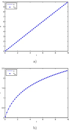
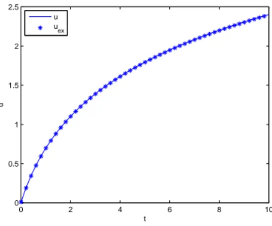
Fig. 2 depicts the computed solution u(t, a). The solution accuracy is quan-tified by comparing the computed solution with the exact one. Fig. 3 compares both solutions in the case of a = 0 (that implies y = 1) and a = 1 (leading to
y = 1 + t). The computed solution is in good agreement with the exact one.
The error calculated using:
E(a) = 1 ∥Ωt∥ ∫ Ωt (u(t, a)− uex(t, a)) 2 dt (54)
was in order of 10−4 by using 10 terms in the finite sums decomposition. The numerical error depends on the time step used in the time discretiza-tion. Tab. 1 shows its evolution with the time step considered whereas Fig. 4
depicts the evolution of the error with the number of terms n in the separated representation of u(t, a). Obviously, this error decreases as the number of terms in the decomposition increases, but it approaches to the error associated to a full tensor product approximation. Further reduction of the error needs the use of finer 1D discretizations (meshes).
∆t 0.01 0.05 0.1 1
E 1 10−5 2.5 10−4 1 10−3 8 10−2
Table 1: Evolution of the error with the time step.
0 0.5 1 1.5 2 0 5 10 0 2 4 6 8 10 a t u
Figure 2: Numerical solution computed by applying the PGD.
4.1.3 Accounting for non-homogeneous initial conditions in local models
In order to enforce non-zero initial conditions the simplest way consists of ap-plying a variable change. Therefore, we define a new unknown ˜u as:
˜
u = u− u0 (55)
where u0is the initial condition. Indeed, enforcing ˜u = 0 is equivalent to enforce u = u0.
Introducing variable change in Eq. (37) the evolution of ˜u is governed by:
y ( d˜u(t, y) dt + du0(t, y) dt )
= 1 ∀t ∈ (0, tmax] ∀y ∈ [ymin, ymax] (56)
But as u0is time independent, the equation becomes:
yd˜u(t, y)
0 2 4 6 8 10 0 1 2 3 4 5 6 7 8 9 10 t u u u ex a) 0 2 4 6 8 10 0 0.5 1 1.5 2 2.5 t u u u ex b)
0 2 4 6 8 10 12 14 10−5 10−4 10−3 10−2 10−1 100 Iteration Error
Figure 4: Error versus the number of sums in the finite sums decomposition.
which doesn’t depend on u0. Thus, just solving this equation is sufficient to
know u for every value of u0 from Eq. (55). Now, the separated representation
based strategy can be used again for solving Eq. (57). In fact, it has already been performed because Eq. (57) is similar to Eq (37).
In a more general case, if u0appears in the equation governing the evolution
of ˜u (after having performed the variable change), we could introduce u0 as a
new model coordinate. Thus, in that case, the separated representation writes:
˜ u(t, y, u0)≈ n ∑ i=1 Ti(t)· Yi(y)· Ui(u0) (58)
This expression is valid because u0 neither depends on time nor on y. The
PGD leads to the solution of u at any t, y, u0, i.e. u(t, y, u0).
The solution can be expressed by: u = f (t, y, u0). When the coordinate y is
time dependent, it could be assumed piecewise constant, linear or polynomial. If we assume a piecewise constant variation, the solution u = f (t, y, u0) could
give the solution at each step of y. If we assume a length ∆tyof the y steps, then
u = f (t, y1, u0) is valid in [0, ∆ty]. Now, if we assume that u1= f (∆ty, y1, u0),
then the solution for the next value of y, y2, is given by: u = f (t− ∆ty, y2, u1)
and so on. Thus, only the solution of the model in the time interval ]0, ∆ty]
is required. Obviously, if ∆ty = ∆t (∆t being the time step used in the time
discretization) there is not computing-time reduction because the number of calculations becomes the same as the one involved in a standard incremental solution. However, if ∆ty >> ∆t, then the computing-time savings can be
significant.
Eqs. (57) and (55) allow computing the solution for all t, y and u0. Now,
we are considering the previous algorithm to build-up the solution for a time evolving parameter. Fig. 5 depicts the computed solution for an evolution of
with the exact solution. The corresponding error is 1.5×10⁻⁵. This solution was computed using ∆ty= ∆t allowing a good accuracy but in fact the solution
is absolutely equivalent to a backward standard time integration. However, when the time evolution of y is smooth enough we can approximate it from a piecewise constant description. Thus, the function y is assumed constant in each interval of length ∆ty >> ∆t defined by a partition t
y
i of the whole time
interval (tyi+1− tyi = ∆ty, t y 0= 0). 0 2 4 6 8 10 0 0.5 1 1.5 2 2.5 t u u u ex
Figure 5: Numerical versus exact solution u(t) with y = 1 + t.
In this case the solution reconstruction from the separated representation
u(t, y, u0) is obtained from:
u(tyi−1≤ t ≤ tyi) = f(t− tyi−1, yi, u(t y i−1)
)
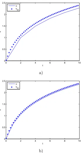
, ∀i ≥ 1 (59) By using this strategy the computing time savings increase as the ratio ∆ty/∆t increases. Fig. 6 compares the computed and the exact solutions for
y = 1 + t and for two different sizes of ∆ty. As expected, the solution accuracy
increases as the number of intervals increases. With 10 intervals (each one containing 20 time steps, i.e. ∆ty = 20· ∆t), the numerical solution fits the
exact one whereas the number of iterations is reduced in the order of 20. The error when using 10 intervals was 2· 10−3 and the one when using 5 intervals was 2· 10−2.
Further improvements can be attained by performing a polynomial approx-imation of y on each interval ∆ty.
In general, the solution of a model depends strongly on the initial condition. This fact motivates the introduction of the initial condition as a new model coordinate. We are now considering a bit more complex problem:
ydu
0 2 4 6 8 10 0 0.5 1 1.5 2 2.5 t u u u ex a) 0 2 4 6 8 10 0 0.5 1 1.5 2 2.5 t u u u ex b)
Figure 6: Numerical versus exact solution of u(t) with y = 1+t: a) ∆ty= 20·∆t;
where h corresponds to a source term that could be also considered unknown or badly known. When h = 0 the exact solution writes:
u = u0exp ( −t y ) (61)
For solving Eq. (60) we introduce a change of variable: ˜
u = u− u0 (62)
which leads to:
yd˜u
dt + ˜u + u0= h with u(t = 0) = 0˜ (63)
Then a separated representation is performed including the coordinates
t, y, u0and the unknown source term h. From this general solution u(t, y, u0, h)
as soon as the different model parameters are given (yg, ug
0, hg) one could extract
the time solution evolution from u(t, yg, ug
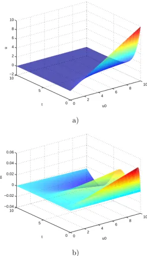
0, hg). Figure 7 depicts the computed
solution u(t, u0) for hg = 0 and yg = 1. The maximum difference between the
computed and the exact solutions never exceeds the value of 0.04 which repre-sents about 0.2% of the solution. Fig. 8 shows similar results for u0 = 5. The
error calculated using Eq. (54) is 8·10−5.
5
Solving non-local non-linear parametric
mod-els
Until now, only local linear problems have been considered, however Proper Generalized Decomposition can be also successfully applied for solving non-local non-linear models. In what follows we are describing the solution of such models defined by parabolic non-linear partial differential equations containing some unknown or badly known parameters.
5.1
Treating non-linearities
For the sake of simplicity we consider the one-dimensional non-linear heat equa-tion: ∂u ∂t − k ∂2u ∂x2 = u 2+ f (t, x) ∀t ∈ Ω t ∀x ∈ Ωx (64)
where u is the temperature field, k is the thermal diffusivity assumed constant and f is a source term. This model is defined in Ωx = (xmin, xmax)× Ωt =
(0, tmax].
The initial condition is:
u(0, x) = 0, ∀x ∈ Ωx (65)
and the boundary conditions are:
0 2 4 6 8 10 0 5 10 −2 0 2 4 6 8 10 u0 t u a) 0 2 4 6 8 10 0 5 10 −0.04 −0.02 0 0.02 0.04 0.06 u0 t u−u ex b)
Figure 7: a) Computed solution u(t, u0). b) Computed and exact solutions
0 2 4 6 8 10 −1 0 1 2 3 4 5 t u u u ex
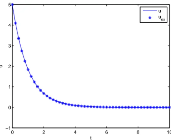
Figure 8: Computed solution u(t, y = 1, u0= 5, h = 0).
The weak formulation results: ∫ Ωt ∫ Ωx u∗ ( ∂u ∂t − k ∂2u ∂x2 − u 2− f ) dΩ = 0 (67)
This section focuses in the treatment of the non linearities, and then all the model parameters are assumed known. Thus, the separated representation of the unknown field writes:
u(t, x) =
∞
∑
i=1
Ti(t)· Xi(x) (68)
For building-up such separated approximation we look at iteration n for the functions R(t) and S(x): u(t, x) = n ∑ i=1 Ti(t)· Xi(x) + R(t)· S(x) = un+ R· S (69)
where functions Ti and Xi were computed at previous iterations.
Different strategies exist for treating the presence of the non-linear term u2. We consider three possibilities:
• The non-linear term is evaluated from the solution at the previous iteration un: u2≈ (un)2= ( n ∑ i=1 Ti· Xi )2 (70)
It is direct to conclude that when the enrichment procedure converges,
∥un− un−1∥ ≤ ϵ, and then ∥(un)2− (un−1)2∥ ≤ ϵ′ that guarantees the
• Another possibility lies in partially using the solution just computed within
the non-linear solver iteration scheme:
u2≈ ( n ∑ i=1 Ti· Xi ) · ( n ∑ i=1 Ti· Xi+ R(t)· S(x) ) (71)
• A third possibility is a variant of the previous one that considers: u2≈ ( n ∑ i=1 Ti· Xi+ R(k−1)· S(k−1) ) ( n ∑ i=1 Ti· Xi+ R(k)· S(k) ) (72)
where k denotes the iteration of the non-linear solver used for computing the enrichment functions R(t) and S(x).
5.1.1 Numerical results
To test the different strategies we consider a problem with a known exact solu-tion.
For this purpose we consider Eq. (64) with the source term:
f (t, x) = (16π2t + 1) sin(4πx)− t2sin(4πx)2 (73) where the exact solution writes:
uex(t, x) = t sin(4πx) (74)
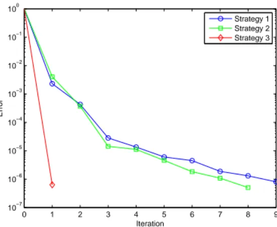
The exact solution (74) involves a single product of space and time functions. The first strategy described in the previous section computes 9 couples of functions. In fact, the number of couples depends more on the efficiency of the linearization strategy than in the separability of the exact solution. The second strategy is expected to give better results because of the better representation of non-linearity. Thus, similar precision was reached with 8 functional couples. Finally, the third strategy computes a single couple of functions for the same precision. Fig. 9 compares the convergence rates of these three strategies.
The third strategy seems to be the best one where the number of functional couples only depends on the separability of the exact solution. However, a computational cost very close to the other ones.
5.2
Non-linear parametric models
In this section we introduce parameters in the model. We consider again the one-dimensional heat transfer equation
∂u ∂t − ∂ ∂x ( k∂u ∂x ) = 0 ∀t ∈ Ωt ∀x ∈ Ωx (75)
where the thermal diffusivity is assumed depending on the temperature field, i.e. k(u):
0 1 2 3 4 5 6 7 8 9 10−7 10−6 10−5 10−4 10−3 10−2 10−1 100 Iteration Error Strategy 1 Strategy 2 Strategy 3
Figure 9: Convergence analysis for the three non-linear solution strategies.
k = au + b (76)
where coefficients a and b are considered as parameters that will be associated to new model coordinates.
Introducing the diffusivity expression into the heat transfer equation (75) we obtain: ∂u ∂t − b ∂2u ∂x2− au ∂2u ∂x2 − a ( ∂u ∂x )2 = 0 (77)
The purpose of the resolution of that equation is the calculation of the temperature at each point and time, and for any value of the parameters a and b within their domains of variability, i.e. u(t, x, a, b):
u(t, x, a, b)≈
n
∑
i=1
Ti(t)· Xi(x)· Ai(a)· Bi(b) (78)
with, in our numerical experiments, t∈ Ωt= (0, 1], x∈ Ωx= (−1, 1), a ∈ Ωa =
[−1, 1] and b ∈ Ωb= [1, 5].
The initial condition writes:
u(t = 0, x, a, b) = 1− x10 (79) and the temperature is assumed vanishing on the boundary of the spatial domain
x =−1 and x = 1.
We consider the approximations of the different functions Ti(t), Xi(x), Ai(a)
and Bi(b) performed by using standard one dimensional linear finite element
shape functions on a uniform mesh consisting of 500 nodes in each 1D-domain Ωt, Ωx, Ωa and Ωb. If this problem is solved using a mesh-based strategy
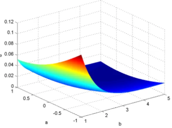
in the whole domain the complexity scales with 5004. However, the Proper Generalized Decomposition needed a single minute using a personal laptop. Fig. 10 illustrates the computed solution for t = 1 and x = 0.
Figure 10: Temperature versus parameters a and b defining the thermal diffu-sivity for t = 1 and x = 0.
6
Conclusion
In this paper we revisited the Proper Generalized Decomposition technique. This discretization strategy is based on the use of a separated representation of the differential operators, the functions and the unknown fields involved in a partial differential equation. The numerical complexity scales linearly with the dimension of the space instead of the expected exponential scaling characteristic of mesh based discretization techniques.
The main advantage lies in the fact that in some models involving unknown or badly known parameters, these parameters could be included as additional coordinates. Despite the fact that the dimension of the model increases, the separated representation allows its efficient and accurate solution. We illustrated this procedure by considering some simple problems where bifurcations are not present. We have also analyzed the solution of non-linear parabolic models, where the eventual presence of uncertain parameters was also incorporated, proving the potentiality of the proper generalized decomposition for addressing complex thermomechanical models encountered in computational mechanics and engineering.
References
[1] Y. Achdou and O. Pironneau. Siam frontiers in applied mathematics.
Com-putational methods for option pricing, 2005.
[2] A. Ammar and F. Chinesta. Circumventing curse of dimensionality in the solution of highly multidimensional models encountered in quantum mechanics using meshfree finite sums decomposition. Lectures Notes on
Computational Science and Engineering, 65:1–17, 2008.
[3] A. Ammar, B. Mokdad, F. Chinesta, and R. Keunings. A new family of solvers for some classes of multidimensional partial differential equa-tions encountered in kinetic theory modelling of complex fluids. J.
Non-Newtonian Fluid Mech., 139:153–176, 2006.
[4] A. Ammar, B. Mokdad, F. Chinesta, and R. Keunings. A new family of solvers for some classes of multidimensional partial differential equations encountered in kinetic theory modelling of complex fluids. part ii: Transient simulation using space-time separated representations. J. Non-Newtonian
Fluid Mech., 144(2-3):98–121, 2007.
[5] A. Ammar, D. Ryckelynck, F. Chinesta, and R. Keunings. On the reduction of kinetic theory models related to finitely extensible dumbbells. J.
Non-Newtonian Fluid Mech., 134:136–147, 2006.
[6] M. Berveiller, B. Sudret, and M. Lemaire. Stochastic finite element: a non-intrusive approach by regression. Eur. J. Comput. Mech., 15:81–92, 2006.
[7] G. Beylkin and M. Mohlenkamp. Algorithms for numerical analysis in high dimensions. SIAM J. Sci. Com., 26(6):2133–2159, 2005.
[8] H.J. Bungartz and M. Griebel. Sparse grids. Acta numerica, 13:1–123, 2004.
[9] R.E. Caflisch. Monte carlo and quasi-monte carlo methods. Acta numerica, 7:1–49, 1998.
[10] E. Canc`es, M. Defranceschi, W. Kutzelnigg, C. Le Bris, and Y. Maday. Computational quantum chemistry: a primer. Handbook of Numerical Analysis, X:3–270, 2003.
[11] F. Chinesta, A. Ammar, and P. Joyot. The nanometric and micrometric scales of the structure and mechanics of materials revisited: An introduc-tion to the challenges of fully deterministic numerical descripintroduc-tions.
Inter-national Journal for Multiscale Computational Engineering, 6(3):191–213,
[12] F. Chinesta, A. Ammar, F. Lemarchand, P. Beauchene, and F. Boust. Alleviating mesh constraints: Model reduction, parallel time integration and high resolution homogenization. Comput. Methods Appl. Mech. Engrg., 197(5):400–413, 2008.
[13] R. Ghanem and P. Spanos. Stochastic finite elements: A spectral approach.
Springer, Berlin, 1991.
[14] P. Ladeveze. Nonlinear computational structural mechanics. Springer, NY., 1999.
[15] R.B. Laughlin. The theory of everything. In Proceeding of the U.S.A
National Academy of Science, 2000.
[16] H.G. Matthies and A. Keese. Galerkin methods for linear and nonlinear elliptic stochastic partial differential equations. Comput. Methods Appl.
Mech. Engrg., 194(12-16):12951331, 2005.
[17] B. Mokdad, E. Pruliere, A. Ammar, and F. Chinesta. On the simulation of kinetic theory models of complex fluids using the fokker-planck approach.
Applied Rheology, 17(2):26494, 1–14, 2007.
[18] A. Nouy. Recent developments in spectral stochastic methods for thenu-merical solution of stochastic partial differential equations. Archives of
Computational Methods in Engineering, In press.
[19] A. Nouy. A generalized spectral decomposition technique to solve a class of linear stochastic partial differential equations. Comput. Methods Appl.
Mech. Engrg., 196:4521–4537, 2007.
[20] M. Papadrakakis and V. Papadopoulos. Robust and efficient methods for stochastic finite element analysis using monte carlo simulation. Comput.
Methods Appl. Mech. Engrg., 134:325–340, 1996.
[21] B. Puig, F. Poirion, and C. Soize. Non-gaussian simulation using hermite polynomial expansion: convergences. Probab. Engrg. Mech., 17:252–264, 2002.
[22] T. M. Rassias and J. Simsa. Finite sums decompositions in mathematical analysis. John Wiley and Sons Inc., 1995.
[23] D. Ryckelynck, F. Chinesta, E. Cueto, and A. Ammar. On the a priori model reduction: overview and recent developements. Archives of compt.