Science Arts & Métiers (SAM)
is an open access repository that collects the work of Arts et Métiers Institute of
Technology researchers and makes it freely available over the web where possible.
This is an author-deposited version published in: https://sam.ensam.eu Handle ID: .http://hdl.handle.net/10985/9297
To cite this version :
Paul BEAUCAIRE, Nicolas GAYTON, Emmanuel DUC, Jean-Yves DANTAN - Statistical tolerance analysis of a mechanism with gaps based on system reliability methods - Procedia CIRP - Vol. 10, p.2-8 - 2013
Any correspondence concerning this service should be sent to the repository Administrator : [email protected]
Statistical tolerance analysis of a mechanism with gaps based on
system reliability methods
P. Beaucaire
a*, N. Gayton
a, E. Duc
a, J.-Y. Dantan
baClermont Université, IFMA, EA3867, LaMI, BP10448, 63000 Clermont-Ferrand, France bLCFC, Arts et Métiers ParisTech Metz, 4 Rue Augustin Fresnel, 57078 Metz Cedex 3, France
One of the aim of statistical tolerance analysis is to evaluate a predicted quality level in the design stage. A method consists in computing the defect probabilityP expressed in parts per million (ppm). It represents the probability that a functional requirement D will not be satisfied in mass production. This paper focuses on the statistical tolerance analysis of over-constrained mechanism with gaps. In this case, the values of the functional characteristics depend on the gap situations, and are not explicitly formulated as a function of part deviations. To computeP , two different methodologies will be presented and confronted. The first one is based on D an optimization algorithm and Monte Carlo simulations. The second methodology uses system reliability methods. The whole approach is illustrated on a basic academic problem inspired by industrial interests.
1. Introductiona
In very competitive industrial fields such as the automotive industry, more and more interest is being paid to the quality level of manufactured mechanisms. It is very important to avoid warranty returns and manage the rate of out-of-tolerance products in production that can lead to assembly line stoppages and/or wastage of out-of-tolerance mechanisms. The quality level of a mechanism can be evaluated by the number of faulty parts in production or by the number of warranty returns per year. However, these two methods of product quality evaluation remain a posteriori. Tolerance analysis is a more interesting way to evaluate a predicted quality level in the design stage. Scholtz [1] proposes a detailed review of classical methods whose goal is to predict functional characteristic variations based on component tolerances. Moreover, statistical tolerance analysis enables the definition of the probability that the functional requirement will be respected or not, as the
well known RSS (Root Sum of Squares) does. Advanced statistical tolerance analysis methods allow the defect probability of an existing design to be computed, knowing the dimension tolerances and functional requirements. Various assumptions about the statistical distributions of component dimensions can be made based on their tolerances and capability levels. For example, the APTA (Advanced Probability-based Tolerance Analysis of products) method proposed by Gayton et al. [2] allows to consider random mean deviations and standard deviations of components statistical distributions. This defect probability, noted
D
P in the following, is expressed in ppm (parts per million). It represents the probability that a functional requirement will not be satisfied in mass production. In a mechanism constituted of several parts, PD is usually computed based on a classical analytical chain of dimensions [3].
For a mechanism with gaps, there exist several potential contact points situations, each one involving a different dimension chain. Thus, the PD formulation and computation are not straightforward. In the literature, gaps are often neglected since only isoconstrained mechanisms are studied. As gaps are present in all
mechanisms in motion, they have to be taken into account. Moreover, they have to be considered as non-probabilized variables since they can not be controlled, but only limited. To study the respect of functional requirements in such mechanisms, all mobilities between parts, arisen from gaps, have to be considered. For this purpose, a new formulation of the tolerance analysis based on the quantifier notion was developed by Dantan
et al. [4]:
The mathematical expression of tolerance analysis for assembly requirement is: “For all acceptable
deviations (deviations which are inside tolerances), there exists a gap situation such as the assembly requirements and the behavior constraints are verified”.
The mathematical expression of tolerance analysis for functional requirement is: “For all acceptable deviations (deviations which are inside tolerances), and for all admissible gap situations, the assembly and functional requirements and the behavior constraints are verified”.
The quantifiers ‘for all” and “there exists” provide a univocal expression of the condition corresponding to a geometrical product requirement. This opens a wide area for research in tolerance analysis. This paper focuses only on the functional requirement issue. Two different methodologies will be presented and confronted in the next sections. Their mutual interest is to take into account all the potential contact points situations. The first one, which has already been used by Dantan et al. [4], considers them at one time. The PD
computation is then based on an optimization algorithm and Monte Carlo simulations. This methodology is very precise in general but requires a lot of optimization runs. It will be presented in Section 2. In the second methodology detailed in Section 3, inspired by the work of Ballu et al. [5], the different situations are identified and considered as dependent events, which are treated separately. Thanks to system reliability methods, a new
D
P formulation is proposed. It is then computed using the n-dimensional multivariate normal distribution n in this paper, commonly employed in system reliability analysis. This methodology decreases largely the computational effort. The whole approach is illustrated on a basic academic problem (Figure 1), inspired by coaxial connectors supplier interests. The results are given and commented in Section 4. Both presented methodologies can be adapted to other mechanisms with gaps.
2. Classical Tolerance analysis issue for mechanisms with gaps
2.1. General formulation for functionality issues
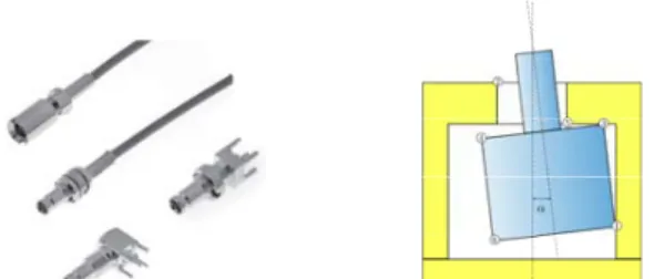
Fig. 1a (left): Industrial coaxial connector. Figure 1b (right): Model of the considered mechanism with gaps. Gaps are emphasized for a better comprehension.
The behavior of a mechanism with gaps is controlled through at least one identified functional characteristic, dependent of two types of variables:
( , )
Fc f D P (1)
Dimensions D of parts are modeled by random
variables where is the hazard. However positions P of parts are modeled by deterministic variables. These variables are not considered as random since displacements of parts cannot be controlled, but only limited by part dimensions.
For functionality issues on mechanisms with gaps, as parts are mobile, the functional requirement must be respected for all admitted positions P of parts. In 3 dimensions, a part has 6 degrees of freedom (3 translations and 3 rotations) which involve 6 displacement variables P. Due to those displacements,
Nc non-interference constraints g D Pj , 0 , corresponding to Nc potential contact points, are defined. They prevent parts from coming into collision with each other. They can be established thanks to different methods: small displacements torsor [6], or directly by considering each potential contact points. They constitute the non-interference domain D
representing the admitted positions P of parts such as they do not collide with each other. The system is functional if: , , , min max : ( , ) 0 1 Fc Fc Fc Nc g j j P D D P D D P (2)
Finally, the goal is to compute the PD probability that functional requirements are not respected. The defect probability is defined as:
min max min max Prob , , , Prob , , < Prob , , > D P Fc Fc Fc Fc Fc Fc Fc D D D P D P P D P P D P (3)
In the next sections, as the two probability terms can be treated similarly, the lower bound Fcmin is not considered.
2.2. Resolution strategy using Monte Carlo simulations and optimization
The defect probability defined above can be computed thanks to the well-known MC (Monte Carlo) simulation method. But, due to gaps, this formulation requires all the admitted positions of parts to be taken into consideration. To ensure that, an optimization algorithm is called for each sample of random variables
D to find the worst functional characteristic value
max(Fc) in regards to the associated functional requirementFcmax. For a given value of D,Fc D P( , ) is maximized under Nc non-interference constraints:
, 0, 1 to
j
g D P j Nc. Finally the defect probability
is written as follows: max ( ) Prob max ( , ) D P Fc Fc P D D P (4) (5)
The algorithm is composed of four steps. The first next three steps are repeated Nl times: k 1 to Nl , where Nl
is the number of MC simulations.
1. A set of dimensions D(k) is randomly decided.
2. Once the non-interference domain k
is constituted, ( ) max , k k Fc P D P is computed
thanks to an optimization algorithm. 3. Indicator ( )k D I is introduced : ( ) max ( ) 1 if max , 0 else k D k k Fc Fc I P D P (5) 4. Finally, PD E ID .
This methodology can be very precise but requires millions of optimization runs to reach small defect probability values, so a second methodology has been developed to reduce the computation time of PD. It will be presented in the next section.
3. A new approach to treat tolerance analysis for mechanisms with gaps issues
3.1. System formulation
As previously said, all the part positions situations have to be taken into consideration. The first methodology is global since it considers all the contact
points at once (i.e. the Nc non-interference constraints). Actually, it is possible to decompose the global defect event into several identified ones, each one relative to a contact points situation. It is the aim of the presented methodology. This approach is called “system” since the problem is composed of a system of events. The advantage of this approach is that gaps disappear for a given contact point situation. It is then much easier to verify the functional requirement respect. A contact point situation is defined such as all freedom degrees are removed, thus 6 non-interference constraints are equal to 0: gi D P, 0, i 1 to 6 . These constraints are linearized thanks to a Taylor expansion around a pertinent point in the P space, function of the application. Since parts positions variations are very low in tolerance analysis problem, the linearized equations
,
j
g D P are very close to the original ones which enable the problem to be treated much more easily. For
each of the 6
Nc
Ns C contact points situations, it is
possible to solve the i-th (i 1 to Ns) linear problem:
, 0, 1 to 6
i j
g j
s D P which solution is ˆPi, where
i j
s is the j-th term of the i
s vector. This vector contains
the identification numbers (i.e. 6 numbers from 1 to Nc)
of the involved non-interference constraints in the i-th
contact point situation. If ˆPiexists, it means that the first six concerned non-interference constraints are respected. Then the other ones making up the non-interference domain have to be checked (i.e. the Nc-6 others). As constraints are linear therefore monotonous, the extreme
Fc value is given by obtaining the maximal functional
characteristic among all individual situations: 6 1 1 ˆ ˆ max , max , , i , 0 j Ns Nc i i i j Fc Fc gs P D D P D P D P
(6) where i j
s is the vector containing the identification
numbers of the non-interference constraints which are not involved in the i-th contact points situation. Thus, according to structural systems reliability theory [7], the original defect probability is transformed as follows:
6 max 1 1 6 1 1 6 1 1 ˆ ˆ Prob max , , , 0 0 ˆ Prob min , , 0 0 ˆ Prob 0 , 0 i j i j i j Ns Nc D i i j Ns Nc i i i j Ns Nc i i j i P Fc Fc g L g L g i s s s D P D P D D P D D P (7)
where performance functions are
max ˆ
( ) ,
i i
L D Fc Fc D P . The problem is thus reduced
to a system problem of Ns unions of Nc-6 intersections
of dependent events. As it is, the PD computation is not trivial. It can be simplified by two aspects. Firstly, the
number Ns of considered situations can be reduced.
Secondly, unions of intersections can be transformed.
3.2. Simplified system formulation
For practical reasons, only a few of the Ns contact
point situations are realistic in the dimensions variations domain. Some of them are mechanically unfeasible. Some are redundant with others. For all these reasons, an identification phase is recommended to get the dominant situations. Ballu et al. [5] do it by knowledge and expertise, but it is not always possible. Another possibility is to run the optimization used in the first methodology a small number of times (100 times for example) in the dimensions variations domain. For each set of dimensions, the optimization algorithm find
max(Fc) while saturating some constraints. Those saturated constraints represent the identified contact point situations which cover defect probabilities. This trick enables to reduce significantly the number Ns of considered events for most of mechanisms. The number of dominant contact point situations is noted Nds. The second simplification step consists in transforming the
D
P formulation thanks to the Poincaré formula:
( ) ( ) ( ) ( ) 6 1 1 6 1 6 1 6 1 1 1 ˆ Prob 0 , 0 ˆ 0 , 0 ... Prob ˆ ... 0 , 0 ... ˆ 1 Prob 0 , 0 c i j c i j c i j c i j Nds N D i i j i N i i j N i k k k j Nds N Nds i i j i P L g L g L g L g s s s s D D P D D P D D P D D P (8)
This formula transforms unions of events intersections into only events intersections. It allows to compute PD
more easily.
3.3. Resolution strategy using FORM system
Several methods such as FORM (First Order Reliability Method) system can treat this kind of system problem very efficiently [8]. Each event (L Di 0 and ( )i ,ˆ 0
j i
g
s D P ) is considered individually by the
classical FORM method. The preliminary task is to transform physical variables D into standard ones U (i.e. Gaussian variables with means and variances respectively equal to 0 and 1). In the case of uncorrelated Gaussian variables, the transformation is
direct: Ui Di i i where i and i are
respectively the means and the standard deviations of random variables D. In other cases this can be more complicated, but the method is well known (see [8] for details). In the new U space, a function ( )G D becomes
( )
H U . Each function H Ui( ), called performance or limit-state function, is linearized at the most probable failure point *
i
P and thus replaced by an hyper-plane (a
straight line in 2 dimensions) whose equation is ( )
i
H U (respectively G Di( ) for G Di( )). This point is the closest from the origin respectful of the constraint
( ) 0
i
H U . Its distance from the origin is noted i and called reliability index. The FORM method provides
also some direction cosines:
i (i)* (i)* i i H U H U where (i)* U is the * i P
point coordinates. Once all limit-states (n) are treated separately, the second stage consists in considering unions or intersections of events, which is the system phase. Let F be the following defect domain:
1 1 / ( ) 0 / ( ) 0 n i i n i i F G H D D U U (9)
Figure 2 illustrates the FORM concepts in a 2-dimensional standard U space. The F domain is greyed out. The dependency of different events, i.e. the orientation of hyper-planes, is taken into account through a covariance matrix defined thanks to direction cosines. The ,i j -thterm of is ( ) ( )
,
i j
ij ,
where , is the scalar product. Finally, the defect probability associated to the F domain is estimated using the n-dimensional multivariate normal distribution n:
1 1 P = Prob ( ) 0 Prob ( ) 0 , n D i i n i i n G G D D (10)
Fig. 2 : Illustration of FORM system principle in the standard space
U1,U2. Three dependent events define the defect domain F which is
In the illustrated case of Figure 2, the defect probability is expressed as follows:
3 1 2 3
P =D { , , }, (11)
nis computed thanks to the Genz method [9] which
evaluates the n-dimensional multivariate normal distribution almost instantaneously. As limit-states functions are replaced by hyper-planes, the method gives only an approximation of PD. Again, due to low part dimensions variations in a tolerance analysis context, this linearization is often very accurate. This method can easily be applied to compute the defect probability given Equation 7, only composed of events intersections.
4. Application
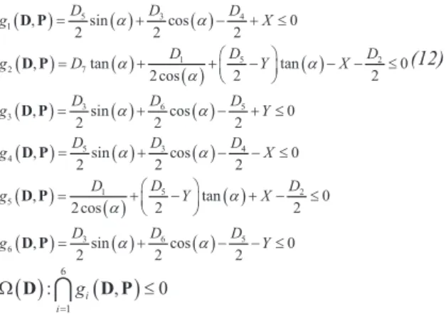
In this section, a case study is presented inspired by industrials interests. It is a two dimensions representation of an electric coaxial connector, constituted by 2 cylindrical parts (see Figure 3). Due to gaps in the mechanism, part 1 is mobile while part 2 is fixed. Position of part 1 is located in the 2D space thanks to the vector of displacement variables: P X Y, , . The rotational symmetry is taken into account by constraining positive. The non-interference domain
D is determined by considering each potential contact points. It depends on the mechanism dimensions and defines the admitted positions and orientation P of part 1:
Fig. 3 : Case study scheme, inspired by an electrical coaxial connector.
5 3 4 1 5 1 2 2 7 3 6 5 3 5 3 4 4 5 1 2 5 3 6 5 6 , sin cos 0 2 2 2 , tan tan 0 2cos 2 2 , sin cos 0 2 2 2 , sin cos 0 2 2 2 , tan 0 2cos 2 2 , sin cos 0 2 2 2 D D D g X D D D g D Y X D D D g Y D D D g X D D D g Y X D D D g Y D P D P D P D P D P D P (12) 6 1 : i , 0 i g D D P
The functional characteristic is Fc . To achieve a correct electrical connection, max, which represents the largest angle admitted by the mechanism, must not exceed a given threshold Fcmax 0.01 rad:
max D PmaxD Fcmax (13)
D characteristics are noted Table 1. They are modeled by
Gaussian variables.
Table 1: Dimension characteristics of the case study.
Name Mean Standard deviation
1 D 6 0.03 2 D 6.1 0.03 3 D 12 0.03 4 D 12.1 0.03 5 D 10.1 0.03 6 D 10 0.03 7 D 3 0.03
To compute PD, the preliminary task is to linearize the initial non-interference constraints g D P, in regards to the displacement space P by using a Taylor expansion around a particular point: X 0, 0, Y Fcmax . This point is very pertinent because Fcmax is the angle at which the functional characteristic value is critical. Then the important contact point situations are identified. They are noted as triplets, which numbers are the contact points identification defined Figure 3. In the 2D space, such a situation has three contact points among the six
ones ( Nc 6 ). As a consequence, there exist
3 6
C 20
Ns potential contact points situations. Five of them are identified in this particular case: {1,2,3}, {1,3,4}, {2,3,6}, {1,3,6} and {2,3,5} as dominant situations. For each of them, a linear problem is solved in order to obtain the P-coordinates ˆP D of those
extreme situations. For example, the first one is defined as follows: 1 1 2 3 , 0 ˆ / , 0 , 0 g g g D P P D P D P D P (14)
Based on this coordinates, 5 performance functions are defined:
max ˆ
( ) , ( ) , 1 to 5
i i
L D Fc Fc D P D i (15)
Those functions, in spite of resulting from a linear system, are not linear in regards to the D space. Thus, the FORM method transforms them into hyper-planes at the most probable failure point. The intersection of events is treated by the FORM system method and PD is computed thanks to the multi-dimensional Gaussian cumulative distributive function n:
5 4 8 1 1 20 ... ... , , ... 1 , D i i ij ij i i j Nds ij Nds ij Nds P (16)
Table 2: Case study results.
Resolution method PD in ppm (95% C.I.) Differences in % Number of calls (computation time) Monte Carlo with non-linear constraints 47329 (257) / 107 optimization runs (3 days) Monte Carlo with linear constraints 47202 (312) 0.6 107 optimization runs (10 hours) FORM system with linear constraints 47245 (225) 0.6 20 FORM resolution (20 seconds)
Where i, ij, ij Nds... i, ij, ij Nds... are the vector of reliability indexes and the covariance matrix associated respectively to the i-th contact points situation (i.e. ( )i ,ˆ 0, 1 to 3
k i
g k
s D P and L Di 0), the i-th
and j-th situations and the Nds situations together. The goal of this application is to show that the problem can be solved at a very low computing cost using the FORM system methodology for simple mechanisms with gaps. Three different resolution methods are proposed based on the two presented methodologies, using both linear and linear non-interference constraints. Results in ppm (parts per million) are listed Table 2 with their 95% confidence
intervals (C.I.). 10 millions runs have been used for MC, so the 95% C.I. width of PD is approximately equal to 300 ppm, ie. 0.6% of results. The FORM system results have also a 95% C.I. due to the Genz method.
The 0.3% difference between the two MC results shows that the non-interference constraints linearization has no measurable impact onPD. Also, as FORM system results are very close to Monte Carlo ones (Table 2), it shows that the FORM linearization phase has no measurable impact either. This argues that the FORM system methodology can deal with this kind of problem with a very low computing cost. To give an idea of the weight of each contact point situations, the individual defect probabilities associated to each situation has been computed as: 3 ( ) 1 ˆ Prob 0 , 0 i D i j i j P L D g D P (17) (1) (2) (3) (4) (5) 30527 65 ppm, 1861 12 ppm 13770 27 ppm, 14781 32 ppm 1 0.01 ppm D D D D D P P P P P (18)
It shows that different situations play a significant role in the defect scenario. Based on these individual situations results, it is possible to compute a PD upper bound:
( ) 1 Nds i D D i P P (19) 5. Conclusion
Statistical tolerance analysis is a key step in the design phase for industrial products. Mechanisms containing gaps are complex because their non conformance is governed by combinations of dependent situations. This paper describes two methodologies: a global one and an innovative one from the structural reliability domain. Instead of using the first costly one, based on Monte Carlo simulations and an optimization, the authors propose to compute the PD defect probability thanks to the FORM system method. Several contact points situations are treated separately as dependent events. Their intersection is taken into consideration thanks to the multi-dimensional Gaussian cumulative distributive function n computed by the Genz method. This innovative methodology requires different functions to be linearized. The industrial application shows that the two presented methodologies give equivalent results and enables the defect probabilities of mechanisms with gaps computation at a very low computing cost. The proposed methodology is remarkably accurate and can be applied on other mechanisms with gaps on which several contact point
situations can be identified to respect functional requirements.
Acknowledgements
The authors would like to thank RADIALL SA, and particularly Laurent Gauvrit, for their cooperation about the presented case study. The Auvergne regional council is also gratefully acknowledged for its financial contribution to this work.
References
[1] Scholtz, F., 1995. Tolerance Stack Analysis Methods. Boeing
Technical Report.
[2] Gayton, N., Beaucaire, P., Bourinet, J.-M., Duc, E., Lemaire, M., Gauvrit, L., 2011. APTA : Advanced Probability-based Tolerance Analysis of products. Mécanique & Industries 12, 71–85.
[3] Nigam, S.D., Turner, J.U., 1995. Review of statistical approaches of tolerance analysis. Computer-Aided Design, vol. 27: pp. 6-15, 1995.
[4] Dantan, J.-Y., Qureshi, A.-J., 2009. Worst-case and statistical tolerance analysis based on quantified constraint satisfaction problems and monte carlo simulation. Computer Aided Design 41, 1–12.
[5] Ballu, A., Plantec, J.Y., Mathieu, L., 2008. Geometrical reliability of overconstrained mechanisms with gaps. CIRP Annals –
Manufacturing Technology 57 (1), 159–162.
[6] Bourdet, P., Mathieu, L., Lartigue, C., 1996. The concept of the small displacement torsor in metrology. Advanced Mathematical
Tools in Metrology II, Series Advances in Mathematics for Applied Sciences: World Scientific, pp. 10-122.
[7] Thoft-Christensen, P., Murotsu, Y., 1986. Application of Structural Systems Reliability Theory. Springer-Verlag.
[8] Lemaire, M., 2009. Structural Reliability. ISTE/Wiley.
[9] Genz, A., 1992. Numerical computation of multivariate normal probabilities. Journal of Computational and Graphical Statistics, 141–149.