HAL Id: hal-03046655
https://hal.archives-ouvertes.fr/hal-03046655
Submitted on 8 Dec 2020HAL is a multi-disciplinary open access archive for the deposit and dissemination of sci-entific research documents, whether they are pub-lished or not. The documents may come from teaching and research institutions in France or abroad, or from public or private research centers.
L’archive ouverte pluridisciplinaire HAL, est destinée au dépôt et à la diffusion de documents scientifiques de niveau recherche, publiés ou non, émanant des établissements d’enseignement et de recherche français ou étrangers, des laboratoires publics ou privés.
Guillaume Aucher
To cite this version:
Guillaume Aucher. Towards Universal Logic: Gaggle Logics. Journal of Applied Logics - IfCoLoG Journal of Logics and their Applications, College Publications, 2020, 7 (6), pp.875-945. �hal-03046655�
Guillaume Aucher Univ Rennes, CNRS, IRISA
263, Avenue du Général Leclerc, 35042 Rennes Cedex, France [email protected]
Abstract
A class of non–classical logics called gaggle logics is introduced, based on a Kripke–style relational semantics and inspired by Dunn’s gaggle theory. These logics deal with connectives of arbitrary arity and we show that they capture a wide range of non–classical logics. In particular, we list the 96 binary con-nectives and 16 unary concon-nectives of basic gaggle logic and relate their truth conditions to the non-classical logics of the literature. We establish connections between gaggle theory and group theory. We show that Dunn’s abstract law of residuation corresponds to an action of transpositions of the symmetric group on the set of connectives of gaggle logics and that Dunn’s families of connec-tives are orbits of the same action. Other operations on connecconnec-tives, such as dual and Boolean negation, are also reformulated in terms of actions of groups and their combination is defined by means of free groups and free products. We show how notions of groups arise naturally from our gaggle logics and how gaggle logics can be canonically defined from given groups. Our other main contribution deals with the proof theory of gaggle logics. We show how sound and complete calculi can be systematically computed from any basic gaggle logic with or without Boolean connectives. These calculi are display calculi and we prove that the cut rule can be systematically eliminated from proofs. This allows us to prove that basic gaggle logics are decidable.
Keywords: substructural logics, residuation, gaggle theory, display cal-culus, group theory, action of group, free group and free product.
1 Introduction
A wide variety of non–classical logics have been introduced over the past decades, such as relevant logics, linear logics and Lambek calculi, to name just a few. On the one hand, this diversity is an asset since each logic has an interest for a specific
purpose, and one can select, and resort to, some of them for reasoning about a given applicative issue [38]. In fact, many of these non–classical logics have been developed for solving concrete problems in computer science: for example, dynamic logics [24], Hoare and separation logics [25, 43] for reasoning about computer programs, and description logics [3] for formalizing ontologies of the semantic web. Acknowledging and dealing with this plurality and diversity of logics is in a sense at the origin of the development of a philosophical stance in logic called “logical pluralism” [5]. On the other hand, and from a theoretical point of view, this plurality can be felt as problematic because it threatens the unity and the unifying power of logic. Indeed, all logics already have in common the same terminology and notions, such as truth, validity, conservativity and interpolation, and this is also an asset. Nevertheless, one can argue that non–classical logics are still disorganized and scattered and somehow miss a common formal ground. As Gabbay summarised the state of play (vis-à-vis non-monotonic logics) in the early 1980s, “we have had a multitude of systems generally accepted as ‘logics’ without a unifying underlying theory and many had semantics without proof theory. Many had proof theory without semantics, though almost all of them were based on some sound intuitions of one form or another. Clearly there was the need for a general unifying framework.” [15, p. 184].
In response to that situation, a number of efforts have been made by some logi-cians to provide a genuine unity to logic as witnessed for example by the development of abstract model theory and “institutions” [4, 33, 19], the introduction of “labelled deductive systems” by Gabbay [17] or the “basic logic” of Sambin & al. [45] (see [16] for details and more examples). This led to the rise of a research thread sometimes referred to (nowadays) as “Universal Logic”. Many kinds of semantics, such as al-gebraic, categorial, topological, phase or relational semantics, have been introduced and developed, sometimes for the express purpose of tackling this issue [46]. Within that line of research, Dunn’s gaggle theory [10, 11, 7] is one of the most well–known frameworks based on the relational Kripke-style semantics which itself deals with the aforementioned problem. Dunn’s gaggle theory is an attempt to understand the Kripke semantics of non-classical logics in a disciplined, systematic way.1
We share the ideal and the objective of “Universal Logic”, but, in our view, gaggle theory is only a first step. Indeed, this theory does not really introduce an actual logic or logical framework that can serve as a foundation for non–classical logics, in the same way as the Lambek calculus is sometimes presented as the foundational logic of the varied substructural logics [42]. However, as we will show, gaggle theory provides formal methods to define a generic logic. In fact, it allows us to define a
1Dunn “owe[s] the name “gaggle” to [his] colleague Paul Eisenberg (a historian of philosophy,
not a logician), who supplied it at [his] request for a name like a “group”, but which suggested a certain amount of complexity and disorder.” [10, p. 31]
class of logics that can handle connectives of arbitrary arity. Building on (partial) gaggle theory, we will define a class of non-classical logics that we call gaggle logics and which generalize the Lambek calculus and other substructural logics in many directions.
In doing so, we will establish connections between gaggle theory and group the-ory. We will show that Dunn’s abstract law of residuation corresponds to an action of transpositions of the symmetric group (the group of permutations) on the set of connectives of gaggle logics and that Dunn’s families of connectives are orbits of the same action. Other operations on connectives, such as dual and Boolean negation, will also be reformulated in terms of actions of groups, and their combination will be defined by means of free groups and free products. We will also show how no-tions of groups arise naturally from our gaggle logics and how gaggle logics can be canonically defined from given groups.
Our other main contribution will deal with the proof theory of gaggle logics. We will show how sound and complete calculi can be systematically computed and defined for any basic gaggle logic given by its set of connectives. This generic result is in line with our ‘universal’ approach explained above and constitutes the main technical advance of the article. We will use a specific Henkin construction method to prove the strong completeness of our calculi. Our main objective is to obtain sound and complete proof calculi for basic gaggle logics without the Boolean connectives. However, we will need to add them anyway and proceed in two steps. Firstly, we will consider a language with the Boolean connectives and prove completeness with them (Section 7). Secondly, after proving the cut elimination (via the proof of conditions (C1) − (C8)), we will obtain sound and complete calculi for basic gaggle logics without the Boolean connectives thanks to a proof-theoretical analysis of the calculi obtained (Sections 8 and 9, proof of Theorem 53). The cut elimination will also entail that basic gaggle logics are conservative extensions of each other and are decidable.
Organization of the article. In Section 2, we recall the basic results of (partial) gaggle theory. In Section 3, we recall the basics of group theory including the symmetric group (the group of permutations), free groups, free products and actions of groups. In Section 4, we introduce our gaggle logics and define our actions of groups on the gaggle connectives, in particular the residuation and the Boolean negation. In Section 5, we prove that Dunn’s abstract laws of residuation are actions of transpositions of the symmetric group on the set of connectives and that Dunn’s families of connectives are orbits of the action of the symmetric group. In Section 6, we relate our gaggle logics with the literature by listing the 96 binary connectives and the 16 unary connectives of basic gaggle logic while mentioning which connectives
have already been introduced in a publication. We also mention two logics which cannot be embedded in gaggle logics. In Section 7, we introduce our display calculi. In Section 8 we prove that our calculi satisfy the display property and that the cut rule can be eliminated from any proof. Then, in Section 9, thanks to cut– elimination, we provide sound and strongly complete display calculi for gaggle logics without Boolean connectives. We also prove that basic gaggle logics are decidable. In Section 10, we show how notions of groups arise naturally from our gaggle logics and how gaggle logics can be canonically defined from given groups. We conclude in Section 11. Long proofs are in the Appendix.
2 The core of gaggle theory
We present the core ideas of (partial) gaggle theory [10, 11]. Partial gaggle first appeared in Dunn [11] as a generalization of a gaggle that has just an underlying poset, not necessarily a distributive lattice as required for a gaggle in Dunn [10]. For our purpose, the presentation of (partial) gaggle theory is slightly different from the usual presentation of this theory. The definitions are the same (although they are sometimes instantiated) but the results of this theory are differently presented. Our results can nevertheless easily be obtained from the original presentation [11].
In this section, we consider given an integer n ∈ N and a non-empty set W. P (W) is the set of subsets of W and if S is a set, Snis the Cartesian product S ×. . .×S, n
times. A n–ary function f on P (W) is a function f ∶ P (W)n→ P (W) and a n–ary
relation R over W is a subset of Wn. We write Rw
1. . . wn for (w1, . . . , wn) ∈ R.
For all m, n ∈ N, the expression Jm; nK denotes the set {m, . . . , n} if m ≤ n, and the empty set � otherwise. In the sequel, we will resort to polarity groups, in particular to the negation group P(+,−) and later to the anti-group P(+,∼).
Definition 1 (Polarity groups). Let (x, y) be an ordered pair. The polarity group associated to (x, y) is P(x,y)� ({x, y}, ⋅) where the operation ⋅ ∶ P(x,y)×P(x,y)→ P(x,y)
is defined by x ⋅ y = y ⋅ x = y and x ⋅ x = y ⋅ y = x. For all ±, ±′∈ {x, y}, we write ±±′
for ± ⋅ ±′.
Note that x is the neutral element of a polarity group.
Definition 2 (Trace, contrapositive trace). A (n–ary) trace is a tuple t = (±1, . . . ,±n,±) ∈ {+, −}n+1, often denoted t = (±1, . . . ,±n) � ±. If j ∈ J1; nK,
then the contrapositive trace of t with respect to its jth argument is the trace
Note that the contrapositive operation on traces is symmetric: �tj�j = t.
Example 3. The 2–ary traces (−, −) � − and (−, +) � + are contrapositive with respect to (w.r.t.) their first argument.
Definition 4 (Relation negation and permutation). Let R be an arbitrary n+1–ary relation over W . Then, for all j ∈ {1, . . . , n}, we define the n + 1–ary relation −R as follows: for all w1, . . . , wn, w∈ W,
−Rw1. . . wnw iff (w1, . . . , wn, w) ∉ R
Sn+1 denotes the set of permutations of the set J1; n + 1K (see Section 3 for
details). If ‡ ∈ Sn+1 is a permutation then its inverse permutation is denoted ‡−.
We define the n + 1–ary relation R‡ as follows: for all w
1, . . . , wn+1∈ W,
R‡w1. . . wn+1 iff Rw‡−(1). . . w‡−(n+1)
We also define +R � R and if ± ∈ {+, −} then R±‡ denotes ±R‡.
Definition 5 (Logical functions associated to a trace and a relation). Let t = (±1, . . . ,±n) � ± be a n–ary trace and let R be a n + 1–ary relation on W. The
n–ary function f on P (W) associated to t and R, denoted fRt, is defined as follows: • If n = 0, ft
R� R;
• If n > 0, then for all W1, . . . , Wn∈ P (W),
fRt(W1, . . . , Wn) � �w ∈ W � CRt (W1, . . . , Wn, w)�
where Ct
R(W1, . . . , Wn, w) is called the truth condition of the function fRt and is
defined as follows:
• if ± = +: “for all w1, . . . , wn ∈ W, we have w1 � W1 or . . . or wn � Wn or
Rw1. . . wnw”;
• if ± = −: “there are w1, . . . , wn ∈ W such that w1 � W1 and . . . and wn � Wn
and Rw1. . . wnw”;
where, for all j ∈ J1; nK, wj� Wj�������
�
wj ∈ Wj if ±j± = +;
wj ∉ Wj if ±j± = −.
Example 6. Let R be a 3–ary relation on W and let ‡ be the permutation (2, 3, 1) on the set J1; 3K (see Section 3 for details). Then, we have that R‡uvw if, and only
• If t = (−, −) � − then the function ft
R ∶ P (W) × P (W) → P (W), whose
truth condition is Ct
R(W1, W2, w) = ∃uv (u ∈ W1∧ v ∈ W2∧ Ruvw), defines the
semantics of a connective, that we denote ○, as follows: for all w ∈ W, w∈ JÏ ○ ÂK iff w ∈ fRt (JÏK, JÂK)
iff ∃uv (u ∈ JÏK ∧ v ∈ JÂK ∧ Ruvw) • If t = (−, +) � + then the function ft
−R‡ ∶ P (W)×P (W) → P (W), whose truth
condition is Ct
−R‡(W1, W2, w) = ∀vu (v ∈ W1∨ u ∈ W2∨ −R‡vuw), defines the
semantics of a connective that we denote �, as follows: for all w ∈ W, w∈ JÏ�ÂK iff w ∈ f−Rt′ ‡(JÏK, JÂK)
iff ∀vu (v ∉ JÏK ∨ u ∈ JÂK ∨ −R‡uvw)
iff ∀vu ((Rwuv ∧ u ∈ JÏK) → v ∈ JÂK) .
Definition 7 (Isotonic and antitonic functions). Let f be a n–ary func-tion on P (W). We say that f is isotonic (resp. antitonic) with respect to the jth argument, written tn(f, j) = + (resp. tn(f, j) = −), when for all
W1, . . . , Wj−1, Wj+1, . . . , Wn, X, Y ∈ P (W),
if X ⊆ Y
then f(W1, . . . , Wj−1, X, Wj+1, . . . , Wn) ⊆ f(W1, . . . , Wj−1, Y, Wj+1, . . . , Wn)
(resp. f(W1, . . . , Wj−1, Y, Wj+1, . . . , Wn) ⊆ f(W1, . . . , Wj−1, X, Wj+1, . . . , Wn)) .
Example 8. If JÏK ⊆ JÏ′K then JÏ′�ÂK ⊆ JÏ�ÂK because tn(ft′
−R‡,1) = −, and JÏ ○ ÂK ⊆
JÏ′○ ÂK because tn(ft
R,1) = +.
Definition 9 (Relation transformations). Let R be an arbitrary n + 1–ary relation over W . Then, for all j ∈ {1, . . . , n}, we define the n + 1–ary relation Rj as follows:
for all w1, . . . , wn, w∈ W,
Rjw1. . . wnwiff Rw1. . . w . . . wnwj
If t = (±1, . . . ,±n) � ± and t′= (±′1, . . . ,±′n) � ±′ are two n–ary traces which are
contrapositive w.r.t. their jth argument, we define the n + 1–ary relation (t′, t)(R)
over W as follows: (t′, t)(R) ���� ��� � Rj if ± = ±′; −Rj otherwise.
Theorem 10. Let R be a n+1–ary relation over W. Let t = (±1, . . . ,±n) � ± and t′=
(±′
1, . . . ,±′n) � ±′ be two contrapositive n–ary traces w.r.t. their jth argument. Let
f (resp. f′) be the n–ary function on P (W) associated to t and R (resp. associated to t′ and (t′, t)(R)). Then, if n > 0:
1. for all j ∈ J1; nK, tn(f, j) = ±j± (and thus tn(f′, j) = ±′j±′ too);
2. f and f′ satisfy the abstract law of residuation w.r.t. their jth argument: for
all W1, . . . , Wn, X∈ P (W), S(f, W1, . . . , Wj, . . . , Wn, X) iff S(f′, W1, . . . , X, . . . , Wn, Wj). where S(f, W1, . . . , Wn, X) ������� � f(W1, . . . , Wn) ⊆ X if ± = − X⊆ f(W1, . . . , Wn) if ± = +.
Example 11. Let us define Ï Â by for all w ∈ W, w ∈ JÏK implies that w ∈ JÂK. Then, the following holds:
• if  Â′ then Ï ○  Ï○ Â′ because tn(fRt,2) = +, and if Ï Ï′ then Ï′� Ï� because tn(f−Rt′ ‡,1) = −. In other words, fRt is isotonic w.r.t. its
second argument and ft′
−R‡ is antitonic w.r.t. its first argument.
• Ï ○  ‰ iff Ï Â�‰, because t and t′ are contrapositive w.r.t. their first argument.
3 Group theory
We first recall some basics of group theory (see for instance [44] for more details). Permutations and cycles. If X is a non-empty set, a permutation is a bijection ‡ ∶ X → X. We denote the set of all permutations of X by SX. In the important
special case when X = {1, . . . , n}, we write Sn instead of SX. Note that �Sn� = n!,
where �Y � denotes the number of elements in a set Y . A permutation ‡ on the set {1, . . . , n} such that ‡(1) = x1, ‡(2) = x2, . . . , ‡(n) = xn is denoted (x1, x2, . . . , xn).
For example, (1, 3, 2) is the permutation ‡ such that ‡(1) = 1, ‡(2) = 3 and ‡(3) = 2. If x ∈ X and ‡ ∈ SX, then ‡ fixes x if ‡(x) = x and ‡ moves x if ‡(x) ≠ x. Let
j1, . . . , jr be distincts integers between 1 and n. If ‡ ∈ Sn fixes the remaining n − r
integers and if ‡(j1) = j2, ‡(j2) = j3, . . . , ‡(jr−1) = jr, ‡(jr) = j1 then ‡ is an r–cycle;
one also says that ‡ is a cycle of length r. Denote ‡ by (j1 j2 . . . jr). A 2–cycle
Two permutations ‡, · ∈ SX are disjoint if every x moved by one is fixed by
the other. A family of permutations ‡1, ‡2, . . . , ‡n is disjoint if each pair of them is
disjoint. Every permutation ‡ ∈ Sn is either a cycle or a product of disjoint cycles.
Moreover, this factorization is unique except for the order in which the factors occur. Groups. A group (G, ○) is a non–empty set G equipped with an associative oper-ation ○ ∶ G×G → G and containing an element denoted 1Gcalled the neutral element
such that:
• 1G○a = a = a○1G for all a ∈ G;
• for every a ∈ G, there is an element b ∈ G such that a○b = 1G= b○a.
This element b is unique and called the inverse of a, denoted a−1. The set S n with
the composition operation is a group called the symmetric group on n letters. A non–empty subset S of a group G is a subgroup of G if s ∈ S implies s−1∈ S
and s, t ∈ S imply s○t ∈ S. In that case, S is also a group in its own right.
If X is a subset of a group G, then the smallest subgroup of G contain-ing X, denoted by �X�, is called the subgroup generated by X. For exam-ple, Sn = �(1 2), (2 3), . . . , (i i + 1), . . . , (n − 1 n)� = �(n 1), (n 2), . . . , (n n − 1)� =
�(n − 1 n), (1 2 . . . n)�. Sn is also generated by (1 2) and 3–cycles. For n ≥ 3,
the alternating group Un is the subgroup of Sn generated by the n–cycles of Sn.
In fact, if X is non–empty, then �X� is the set of all the words on X, that is, elements of G of the form x±11 x±22 . . . x±n
n where x1, . . . , xn ∈ X and ±1, . . . ,±n are
either −1 or empty.
Free groups and free products. If X is a subset of a group F , then F is a free group with basis X if, for every group G and every function f ∶ X → G, there exists a unique homomorphism Ï ∶ F → G extending f. One can prove that a free group with basis X always exists and that X generates F . We therefore use the notation F = �X� also for free groups.
If G and H are groups, the free product of G and H is a group P and homomor-phisms jG and jH such that, for every group Q and all homomorphisms fG∶ G → Q
and fH ∶ H → Q, there exists a unique homomorphism Ï ∶ P → Q with ÏjG = fG
and ÏjH = fH. Such a group always exists and it is unique modulo isomorphism,
we denote it G ∗ H. This definition can be generalized canonically to the case of a finite number of groups G1, . . . , Gn, yielding the free product G1∗ . . . ∗ Gn.
Group actions. If X is a set and G a group, an action of G on X is a function –∶ G × X → X given by (g, x) � gx such that:
• 1x = x for all x ∈ X;
• (g1g2)x = g1(g2x) for all x ∈ X and all g1, g2∈ G.
An action of G on X is transitive if for every x, y ∈ X, there exists g ∈ G such that y= gx; it is faithful if for gx = x for all x ∈ X implies that g = 1.
If x ∈ X and – an action of a group G on X, then the orbit of x under – is O–(x) � {–(g, x) � g ∈ G}. The orbits form a partition of X. The stabilizer of x,
denoted by Gx, is the subgroup Gx � {g ∈ G � gx = x} of G. If G is finite, then we
have that �O–(x)� = �G�G�x�. Moreover, if X and G are finite then the number N of
orbits of X is N = 1
�G�∑·∈GF(·) where, for · ∈ G, F(·) is the number of x ∈ X fixed
by · (Burnside’s lemma). Finally, if X′⊆ X then O
–(X′) denotes � x′∈X′O–(x
′).
Fact 12. If – is an action of G on a set X and H is a subgroup of G, then the restriction of – to H, denoted –H, is also an action of H on the set X.
Definition 13. Let G and H be two groups. If – and — are actions of G and H on a set X, then the free action – ∗ — is the mapping – ∗ — ∶ G ∗ H × X → X given by –∗—(g, x) � –(g1, —(h1, . . . , –(gn, —(hn, x)))), where g = g1h1. . . gnhnis the
factorization of g in the free group G ∗ H.
This definition can be generalized canonically to the case of a finite number of actions –1, . . . , –n, yielding the mapping –1∗ . . . ∗ –n.
Proposition 14. If –1, . . . , –n are actions of G1, . . . , Gn on a set X respectively,
then the mapping –1∗ . . . ∗ –n is an action of the (free) group G1∗ . . . ∗ Gn on X.
4 From gaggle theory to gaggle logics
The introduction of the formal concepts of gaggle theory are motivated by some heuristic and logical reasons (see for example [41] for informal explanations). We are going to reformulate these formal concepts of gaggle theory because we want to make more clear the connection between traces and the relational Kripke–style semantics that they induce. Thereby, we replace the notion of trace by our notion of ‘signature’ which highlights and distinguishes in a more immediate way the different semantic ingredients that compose gaggle theory. More specifically, the output of a trace (+ or −) is replaced by a quantification signature (∀ or ∃). Doing so, our reformulation will capture and represent more directly and faithfully the tonicity of the connective defined by a given trace/signature and the formulation of its truth
condition (even if, as we said, the notion of trace output was introduced for different heuristic reasons [41]).
In this section, we show how gaggle theory, and in particular Definition 5, leads to the definition of finite families of connectives of arbitrary arities which are related to each other by the abstract law of residuation of Theorem 10.
4.1 From traces to gaggle connectives
Informally, ∀ is associated with + and ∃ is associated with −. We formalize this association with the function ± ∶ {∀, ∃} → {+, −} defined by ±(∀) � +, ±(∃) � − and the inverse function Æ ∶ {+, −} → {∀, ∃} defined by Æ(+) � ∀, Æ(−) � ∃. Also, we define the function + ∶ {∀, ∃} → {∀, ∃} by +(∀) � ∀ and +(∃) � ∃ and the function − ∶ {∀, ∃} → {∀, ∃} by −(∀) � ∃ and −(∃) � (∀). For better readability, we write +∀, +∃, −∀, −∃ instead of −(∀), +(∃), −(∀), −(∃).
Definition 15 (Signatures versus traces). A (n–ary) signature s is a tuple s = (Æ, (±1, . . . ,±n)) ∈ {∀, ∃}×{+, −}n. If s = (Æ, (±1, . . . ,±n)) is a n–ary signature and
t= (±1, . . . ,±n,±) a n–ary trace, then
• The trace T (s) equivalent to s is the trace (±′
1, . . . ,±′n) � ± where ± � ±(Æ)
and ±′
j� ±±j for all j ∈ J1; nK.
• The signature S(t) equivalent to t is the signature (Æ, (±′
1, . . . ,±′n)) where
Æ � Æ(±) and ±′
j � ±±j for all j ∈ J1; nK.
Note that the derived notion of tonicity tn(f, j) determined in Theorem 10 is now taken as primitive with our notion of signature. Then, we can easily prove the following:
s= S(T(s)) t= T(S(t))
We also reformulate the definition of contrapositive trace in terms of signature as follows. If s = (Æ, (±1, . . . ,±n)) is a n–ary signature and rj = (n+1 j) a transposition
with j ∈ J1; nK, then we define
rjs� (− ±jÆ, (− ±j±1, . . . ,±j, . . . ,− ±j±n)). (1)
Then, we can easily prove the following: for all n–ary traces t and n–ary signa-tures s,
Moreover, for every cycle c fixing n + 1, we define
cs� �Æ, �±c(1),±c(2), . . . ,±c(n)�� . (2)
This definition is coherent with Expression (1). Indeed, the transpositions (n + 1 1), (n+1 2), . . . , (n+1 n) generate Sn+1and every cycle fixing n+1 can be factorized
into a sequence of transpositions of the form (n + 1 j) so that, applying iteratively Expression (1), we obtain Expression (2).
Definition 16 (Gaggle connectives). The set of atoms P and connectives C are: P �S1× {+, −} × {∀, ∃} C �P ∪ �
n∈N∗
Sn+1× {+, −} × {{∀, ∃} × {+, −}n} .
Both atoms and connectives can be represented by triples p = (1, ±, Æ) (for atoms) and � = (‡, ±, (Æ, (±1, . . . ,±n))) (for connectives) where ‡ ∈ Sn+1, ± ∈ {+, −}
and (Æ, (±1, . . . ,±n)) ∈ {∀, ∃} × {+, −}n. The arity of an atom is 0, the arity of
a connective � = (‡, ±, (Æ, (±1, . . . ,±n))) ∈ C, denoted a(�), is n, its signature
is (Æ, (±1, . . . ,±n)), its quantification signature is Æ and its tonicity signature is
(±1, . . . ,±n). For all j ∈ J1; nK, tn(�, j) denotes ±j. Atoms are denoted p, p1, p2, etc.
and connectives are denoted �, �1,�2, etc. The set of n–ary connectives, for n > 0,
is denoted Cn.
Fact 17. The number of n–ary gaggle connectives is (n + 1)! ⋅ 2n+2.
Proof: It follows from the very definition of connectives. �
4.2 Actions of groups on gaggle connectives
In this section, we introduce actions on the set of gaggle connectives. In the next sections, we will show that they generalize standard notions of residuations, duals and Boolean negation.
Definition 18 (Action of the symmetric group). Let n ∈ N∗. We define the
function –n ∶ Sn+1 × Cn → Cn,(·, �) � ·� inductively as follows. Let � =
(‡, ±, (Æ, (±1, . . . ,±n))) ∈ Cn and let c ∈ Sn+1.
• If c is the transposition rj = (j n + 1), then rj� � (rj○ ‡, − ±j±, rjs), i.e.:
rj� � ((j n + 1) ○ ‡, − ±j±, (− ±jÆ, (− ±j±1, . . . ,±j, . . . ,− ±j±n)) .
Permutations of S2 1–ary signatures
·1 = (1, 2) t1= (∃, +)
·2 = (2, 1) t2= (∀, +)
t3= (∀, −)
t4= (∃, −)
Permutations of S3 2–ary signatures
‡1 = (1, 2, 3) s1 = (∃, (+, +)) ‡2 = (3, 2, 1) s2 = (∀, (+, −)) ‡3 = (3, 1, 2) s3 = (∀, (−, +)) ‡4 = (2, 1, 3) s4 = (∀, (+, +)) ‡5 = (2, 3, 1) s5 = (∃, (+, −)) ‡6 = (1, 3, 2) s6 = (∃, (−, +)) s7 = (∃, (−, −)) s8 = (∀, (−, −))
Figure 1: Permutations of S2 and S3 and ‘families’ of 1–ary and 2–ary signatures
• If c is the cycle (j1 j2 . . . jk n+ 1), then c� � rj1(rj2. . .(rjk�)), where
rj � (j n + 1) for all j.
• If c is a cycle fixing n + 1, then c� � (c ○ ‡, ±, cs), i.e.: c� � �c ○ ‡, ±, �Æ, �±c(1),±c(2), . . . ,±c(n)��� .
Finally, if · is an arbitrary permutation of Sn+1, it can be factorized into a product
of disjoint cycles · = c1c2. . . ck and this factorization is unique (modulo its order)
[44]. So, we define ·� � c1(c2. . .(ck�)).
The mapping –n is well-defined because one can easily prove that any other
ordering of the disjoint cycles c1, . . . , ck of · yields the same outcome for ·�. Our
definition is based on cycles and not on transpositions because the decomposition of any permutation into disjoint cycles is unique (modulo its order), unlike its decom-position into transdecom-positions.
Proposition 19. For all n ∈ N∗, the mapping –
n∶ Sn+1×Cn→ Cn is a group action
of Sn+1 on Cn. For all n ∈ N∗, the group actions –n (and all their restrictions to
subgroups G) are not transitive, the cardinality of each orbit is �Sn+1� (resp. �G�) and
the number of orbits is 4 ⋅ 2n (resp. �Cn�
Proof: (sketch) The condition (·1○ ·2)� = ·1(·2�) of the definition of group actions
is proved by induction on ·1. The other results follow from group theory because
for all x ∈ Cn, Gx= {1}. �
Definition 20 (Actions of the negation group and the anti-group). Let n ∈ N∗.
We define the functions —n ∶ P(+,−)× Cn → Cn,(±, �) � ±� and “n ∶ P(+,∼)× Cn→
Cn,(±, �) � ±� as follows: if � = (‡, ±, (Æ, (±1, . . . ,±n))) ∈ Cn, then
• +� � �
• ∼ � � (‡, −±, (Æ, (±1, . . . ,±n)))
• −� � (‡, −±, (−Æ, (−±1, . . . ,−±n))).
−� and ∼ � are called the Boolean negation and the symmetry of � respectively. Moreover, if � is an atom p = (1, ±, Æ), then we also define −p � (1, −±, −Æ). As we will see in Proposition 29, our definition of Boolean negation does corre-spond to the intended (Boolean) negation.
Proposition 21. For all n ∈ N∗, the functions —
nand “n are non–transitive actions.
For both actions, the cardinality of each orbit is 2 and the number of orbits is �Cn�
2 .
Proof: It follows from the application of Burnside Lemma. Only + fixes connectives of Cnand it fixes all of them. − and ∼ do not fix any element of Cn. �
4.3 Gaggle logics
Our introduction of ‘gaggle logics’, like many semantic-based logics, is made in three parts: first, we define their language (Definition 22), then their class of models (Definition 24) and finally their satisfaction relation (Definition 25).
Definition 22 ((Boolean) gaggle language). The gaggle language L0 is the
small-est set that contains the propositional letters and that is closed under the gaggle connectives. That is,
• P ⊆ L0;
• for all � ∈ C of arity n > 0 and for all Ï1, . . . , Ïn∈ L0, we have �(Ï1, . . . , Ïn) ∈
The Boolean gaggle language L is the smallest set that contains the proposi-tional letters and that is closed under the gaggle connectives as well as the Boolean connectives ∧, ∨ and ¬.
Elements of L are called formulas and are denoted Ï, Â, –, . . . For all Ï1, . . . , Ïn ∈ L, Ï1∧ . . . ∧ Ïn and Ï1∨ . . . ∨ Ïn stand for ((Ï1∧ Ï2) ∧ . . . ∧ Ïn) and
((Ï1∨ Ï2) ∨ . . . ∨ Ïn) respectively.
If C ⊆ C ∪ {∧, ∨, ¬} is such that C ∩ P ≠ �, then an element of LC is an element
of L that contains only connectives and atoms of C. In the sequel, we assume that all the sets of atoms and connectives C ⊆ C ∪ {∧, ∨, ¬} are such that C ∩ P ≠ �. Remark 23. We could consider a countable number of copies of the atoms and connectives: P′� �
i∈N{�i� � ∈ P}, C ′� �
i∈N{�i� � ∈ C}. Indeed, in general we need a
countable number of atoms or, like in some modal logics, we need multiple modalities of the same (similarity) type. All the results that follow would still hold in this extended language.
Definition 24 (C–models and C–frames). Let C ⊆ C. A C–model is a tuple M = (W, R) where W is a non-empty set and R is a set of relations over W. Each n–ary connective � ∈ C is associated to a n+1–ary relation R�such that for all connectives
�1,�2∈ C, we have that R�1 = R�2 iff O–n∗—n(�1) = O–n∗—n(�2).
We abusively write w ∈ M for w ∈ W. A pointed C–model (M, w) is a C–model M together with a state w ∈ M. The class of all pointed C–models is denoted MC
and simply M when C = C. A C–frame is a C�P–model. The class of all pointed C–frames is denoted FC and simply F when C = C.
Definition 25 (Gaggle logics). Let C ⊆ C and let M = (W, R) be a C–model. We define the interpretation function of LC in M, denoted J⋅KM ∶ LC → P (W),
inductively as follows: for all p ∈ C ∩ P and all � ∈ C of arity n > 0 and signature denoted (‡, ±, s), for all Ï, Â, Ï1, . . . , Ïn∈ LC,
JpKM � ±R p J¬ÏKM � W − JÏKM J(Ï ∧ Â)KM � JÏKM ∩ JÂKM J(Ï ∨ Â)KM � JÏKM ∪ JÂKM J�(Ï1, . . . , Ïn)KM � f�(JÏ1KM, . . . ,JÏnKM)
where the function f� = fRt±‡� with t = T(s) defined in Section 4.1 and fRt±‡�
in Definition 5. That is, f� is defined as follows: for all W1, . . . , Wn ∈ P (W),
f�(W1, . . . , Wn) � {w ∈ W � C�(W1, . . . , Wn, w)} where C�(W1, . . . , Wn, w) is called
• if Æ = ∀: “∀w1, . . . , wn∈ W (w1� W1∨ . . . ∨ wn� Wn∨ R±‡� w1. . . wnw)”;
• if Æ = ∃: “∃w1, . . . , wn∈ W (w1� W1∧ . . . ∧ wn� Wn∧ R±‡� w1. . . wnw)”;
where, for all j ∈ J1; nK, wj � Wj � wj ∈ Wj if ±j = + and wj � Wj � wj ∉ Wj if
±j = − and R�±‡w1. . . wn+1 iff ±R�w‡−(1). . . w‡−(n+1) (we recall that +R� � R� and
−R�� Wn+1− R�).
We extend the definition of the interpretation function J⋅KM to C–frames as
fol-lows: for all Ï ∈ LC and all C–frames F ,
JÏKF � ��JÏK(F,P)� P a set of n–ary relations over Wsuch that (F, P) is a C–model� If EC is a class of pointed C–models or C–frames, the satisfaction relation ⊆
EC× LC is defined as follows: for all Ï ∈ LC and all (M, w) ∈ EC, ((M, w), Ï) ∈
iff w ∈ JÏKM. We usually write (M, w) Ïinstead of ((M, w), Ï) ∈ . The triple
(LC,EC, ) is a logic called the gaggle logic associated to EC and C. The logics of
the form (LC,MC, ) are called basic gaggle logics. We call them Boolean (basic) gaggle logics when their language includes the Boolean connectives ∧, ∨, ¬.
The truth conditions of the above definitions have been introduced in a different formal approach by Bimbó & Dunn [7] and for some particular cases by Dunn [10] and Dunn & Hardegree [13]. However, it is the first time that they are spelled out systematically and in a comprehensive manner.
Example 26 (Lambek calculus, modal logic). The Lambek calculus (LC,MC, )
where C = {p, ○, �, �} defined in Section 2 is an example of basic gaggle logic. Here ○, �, � are the connectives (‡1,+, s1), (‡5,−, s3), (‡3,−, s2). Another example of gaggle
logic is modal logic (LC,EC, ) where C = {p, �, �, ∧, ∨, �, �} is such that
• �, � are the connectives (1, +, ∃) and (1, −, ∀) respectively;
• ∧, ∨, �, � are the connectives (‡1,+, s1), (‡1,−, s4), (·2,+, s1), (·2,−, s2)
respec-tively;
• the C-models M = (W, R) ∈ EC are such that R∧= R∨= {(w, w, w) � w ∈ W},
R�= R�, R�= R�= W.
Indeed, one can easily show that, with these conditions on the C–models of EC,
we have that for all (M, w) ∈ EC, (M, w) (‡1,+, s1)(Ï, Â) iff (M, w) Ï and
(M, w) Â, and (M, w) (‡1,−, s4)(Ï, Â) iff (M, w) Ï or (M, w) Â. Note that
the Boolean conjunction and disjunction ∧ and ∨ are defined using the connectives of C by means of special relations R∧ and R∨. They could obviously be defined
5 Residual, Boolean negation, dual and switch
The action of specific permutations on the set of connectives corresponds to well– known operations used in proof theory. For example, the action of a transposition (j n + 1) corresponds to the abstract law of residuation for the jth argument. This
operation of residuation turns out to be central since every permutation can be decomposed into a composition of transpositions. Yet, we argue that the actions of cycles is more central because every permutation can be decomposed uniquely into disjoint cycles. Moreover, the symmetric group Sn+1 is also generated by the cycles
(1 . . . n+1) and (n n+1) and the alternation group is generated by the n+1-cycles of Sn+1. This confirms an observation already made in [2] which highlighted the
role of 3-cycles for substructural and update logics in the formal connections that exist between connectives.
Proposition 27. Let t be a n-ary trace, R a n+1-ary relation over W and ‡ ∈ Sn+1.
Then, ft
R±‡ = f� where � = (‡, ±, S(t)) = (‡, ±, (Æ, (±1, . . . ,±n))). Moreover, if
j ∈ J1; nK, then the n-ary function associated to tj and (tj, t)(R) of Definition 5 is frj� where rj�, the residual of � w.r.t. its j
th argument, was defined in Definition
18:
rj� � ((j n + 1) ○ ‡, − ±j±, (− ±jÆ, (− ±j±1, . . . ,±j, . . . ,− ±j±n)) .
Therefore, we have the following property: for all Ï1, . . . , Ïj, . . . , Ïn, Ï∈ L,
S[�, Ï1, . . . , Ïj, . . . , Ïn, Ï] iff S[rj�, Ï1, . . . , Ï, . . . , Ïn, Ïj] (3) where S [�, Ï1, . . . , Ïn, Ï] ������� � �(Ï1, . . . , Ïn) Ï if Æ = ∃ Ï � (Ï1, . . . , Ïn) if Æ = ∀ .
Proof: It follows straightforwardly from our definitions. Expression (3) follows
from Theorem 10 (item 2). �
Hence, rj� does correspond to the residual connective of � w.r.t. its jthargument
as it is usually defined in Dunn’s theory.
Definition 28 (Dual and switch operations). Let � = (‡, ±, (Æ, (±1, . . . ,±n))) ∈ C
be a n–ary connective and let j ∈ J1; nK.
• The switch of � w.r.t. its jth argument is the n-ary connective
• The dual of � w.r.t. its jth argument is the n–ary connective
dj� � (‡, −±, (−Æ, (−±1, . . . ,±j, . . . ,−±n))).
• The dual of � is the n-ary connective
d� � (‡, −±, (−Æ, (±1, . . . ,±n))).
The following proposition shows that our terminology for “Boolean negation” and “dual” is appropriate and does correspond to the standard intuitive meaning (see Blackburn & Al. [8, Def 1.13] for example).
Proposition 29. Let � ∈ C be a n–ary connective and let Ï1, . . . , Ïn∈ L. Then, for
all (appropriate) pointed models (M, w),
(M, w) − �(Ï1, . . . , Ïn) iff (M, w) � (Ï1, . . . , Ïn) does not hold
(M, w) sj� (Ï1, . . . , Ïn) iff (M, w) � (Ï1, . . . ,¬Ïj, . . . , Ïn)
(M, w) dj� (Ï1, . . . , Ïn) iff (M, w) − �(Ï1, . . . ,¬Ïj, . . . , Ïn)
(M, w) d� (Ï1, . . . , Ïn) iff (M, w) − �(¬Ï1, . . . ,¬Ïn)
The following proposition shows that the switch as well as the dual operations are definable in terms of residuations and Boolean negation.
Proposition 30. If � ∈ Cn is a n–ary connective, then for all j ∈ J1; nK,
• sj� = rj− rj�
• dj� = rj− rj− �
• d� = s1. . . sn− �.
Proof: See the Appendix, Section A. �
Proposition 31. Dunn’s (complete) families of n–ary connectives are orbits O–n(�)
of the group action –n. These families/orbits form a partition of the set of n–ary
connectives.
Proof: It follows easily from Dunn’s and our definitions. � Dunn’s families of n–ary connectives are called “complete families” of operations by Bimbó & Dunn [7]. Likewise, two n–ary connectives �, � ∈ Cn are “colligated”
(‡6,+, s5) (‡6,−, s3) (‡1,+, s1) (‡1,−, s8) (‡6,−, s8) (‡6,+, s1) (‡1,−, s3) (‡1,+, s5) residuation r2 Boolean negation −
Figure 2: The 8 connectives of the orbit O–G2((‡1,+, s1))
(‡1,+, s1) (‡6,−, s3) (‡5,−, s3) (‡4,+, s1) (‡3,−, s2) (‡2,−, s2) residuation r2 residuation r1
Figure 3: The 6 connectives of the orbit O–2((‡1,+, s1))
Proposition 32. Let n ∈ N∗, j ∈ J1; nK and let us define G
j = �rj�∗P(+,−). Since Gj
is a subgroup of Sn+1∗ P(+,−), let us denote by –Gj the action of Gj on Cn induced
by the free action –n∗ —n. Then, for all connectives � of arity n,
1. O–Gj (�) is isomorphic to a cyclic group of order 8.
2. �O–n∗—n(�) , O–n∗—n(∼ �)� forms a partition of the set Cn of connectives of
arity n. Moreover, the mapping ∼⋅ ∶ O–n∗—n(�) → O–n∗—n(∼ �), x �∼ x is
(‡1,+, s1) (‡1,+, s5) (‡1,+, s7) (‡1,+, s6) (‡1,−, s8) (‡1,−, s3) (‡1,−, s4) (‡1,−, s2) (‡6,−, s3) (‡6,+, s5) (‡6,+, s7) (‡6,−, s4) (‡6,−, s8) (‡6,+, s1) (‡6,+, s6) (‡6,+, s2) (‡5,−, s3) (‡5,−, s4) (‡5,+, s7) (‡5,+, s5) (‡5,−, s8) (‡5,−, s2) (‡5,+, s6) (‡5,+, s1) (‡4,+, s1) (‡4,+, s6) (‡4,+, s7) (‡4,+, s5) (‡4,−, s8) (‡4,−, s2) (‡4,−, s4) (‡4,−, s3) (‡3,−, s2) (‡3,+, s6) (‡3,+, s7) (‡3,−, s4) (‡3,−, s8) (‡3,+, s1) (‡3,+, s5) (‡3,−, s3) (‡2,−, s2) (‡2,−, s4) (‡2,+, s7) (‡2,+, s6) (‡2,−, s8) (‡2,−, s3) (‡2,+, s5) (‡2,+, s3) residual r2 residual r1 switch s1 switch s2 negation −
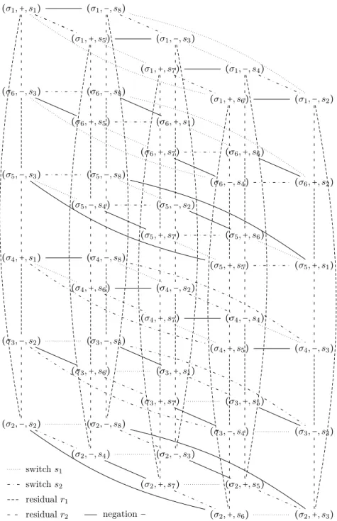
Figure 4: The 48 connectives of the orbit O–2∗—2((‡1,+, s1)) related to each other
3. For all n ∈ N∗, the free action –
n∗ —n∗ “n on the set of connectives Cn is
transitive.
Proof: See the Appendix, Section A. �
So, for every pair of connectives (�, �′), there exists a sequence of residuation(s),
negation(s) and symmetry which transforms � into �′. In other words, every gaggle
connective � ∈ Cn can be obtained from another connective �′∈ Cn with a suitable
choice of element in the free groups Sn+1∗ P(+,−)∗ P(+,∼): for all �, �′∈ Cn, there is
g∈ Sn+1∗ P(+,−)∗ P(+,∼) such that �′= –n∗ —n∗ “n(g, �).
Example 33. In Figure 2, we represent the orbit O–G2((‡1,+, s1)). It is isomorphic
to a group of order 8 according to the first item of Proposition 32. In Figure 4, we represent the orbit O–2∗—2((‡1,+, s1)) where the 48 binary connectives are related
to each other by means of residuation, switch or Boolean negation. The other 48 binary connectives of the orbit O–2∗—2(∼ (‡1,+, s1)) are obtained symmetrically by
switching everywhere − to + and + to −. These two orbits form a partition of C2
according to the second item of Proposition 32. The orbits O–2(�) of the binary
connectives � of C2are given in Figures 7, 8, 9, 10, 11 and 12. Every orbit O–2(�) is
of cardinality 6 = �S3�. In order to follow common notations, binary connectives are
denoted Ï� instead of �(Ï, Â). Finally, the orbit of O–2((‡1,+, s1)) is represented
graphically in Figure 3, it corresponds to the outermost left vertical line of Figure 4.
6 Gaggle logics in the literature
In this section, we provide formal connections between our gaggle logics and sub-structural and non-classical logics. The last columns of our tables indicate the rele-vant publication where the gaggle logic connective was introduced for the first time. A logic close to our approach with connectives of arbitrary arity is the Generalized Lambek Calculus of Kolowska-Gawiejnovicz [26]. It is in fact the basic gaggle logic (LC,MC, ) where C = �
n∈N∗{�n
, ri�n�, i = 1, . . . , n} with �nthe n-ary connnective
(1, +, (∃, (+, . . . , +))). (�n and ri�n are denoted f and f�i in [26].)
6.1 Binary and unary connectives of basic gaggle logic
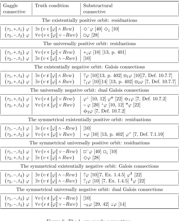
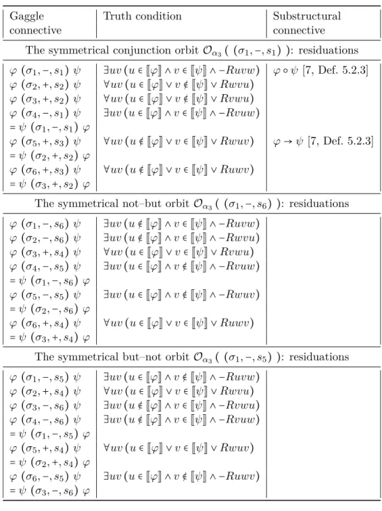
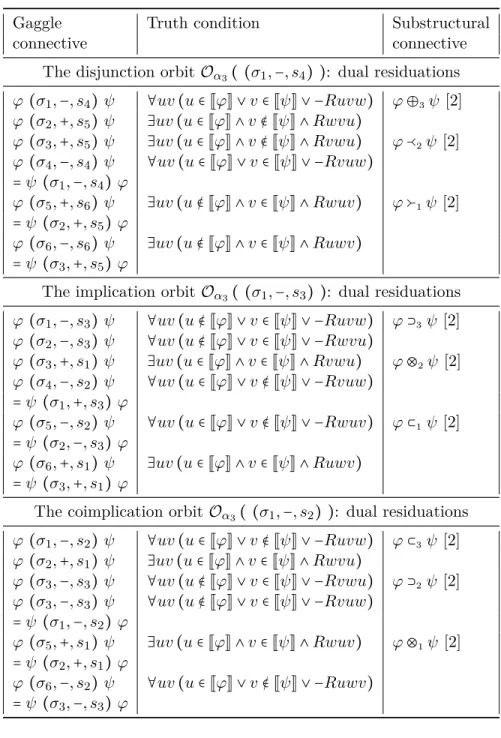
The truth conditions of the 16 unary gaggle connectives of gaggle logic are given in Figure 6 and those of the 96 binary gaggle connectives of gaggle logic in Figures 7, 8, 9, 10, 11 and 12. Many of these unary and binary connectives have already
been introduced in the literature [30, 23, 28, 29, 40, 31, 22, 42, 2]. For example, the binary connectives (‡1,+, s1) , (‡5, s3,−) and (‡3, s2,−) are the fusion ○, implication
� and co-implication � connectives of the Lambek calculus [30] used to illustrate our examples in Section 2. They are also denoted ⊗3, ⊃1 and ⊂2 in update logic
[2].2 In the third column of the tables, we provide the bibliographical references
where the connectives were first introduced. Note that each binary connective � has a commutative version �′ which belongs to the same orbit/family so that for
all formulas Ï, Â we have that Ï � Â = Â �′Ï. So, instead of 6 different connectives
for each 2–ary orbit, we genuinely have 3 different connectives. This is in line with a result about colligated operations of Bimbó & Dunn [7]. For each orbit, one goes from one connective to the next by alternating residuations w.r.t. the first or the second argument, like in Figure 3. For example, (‡1,+, s1) = r1 (‡2,−, s2) =
r1r2 (‡3,−, s2) = r1r2r1 (‡4,+, s1) = r1r2r1r2 (‡5,−, s3) = r1r2r1r2r1 (‡6,−, s3) .
To each family/orbit of connectives corresponds a series of laws of residuation. These laws are all instances of the same abstract law of residuation of Definition 10 and correspond to the action of transpositions of the form (j n + 1) on the set of connectives. They are of different types depending on the family/orbit to which they belong. These types were denoted in the literature: residuation connection, dual residuation connection, Galois connection and dual Galois connection (denoted rp, drp, gc and dgc by Goré [22]). These different ‘types’ of instance of the same abstract law of residuation for binary and unary connectives are given in Figure 5. In particular, note that the notion of dual residuation is the same as our definition of dual w.r.t. the jth argument (Definition 28 and Proposition 29).
6.2 Non gaggle logics
Some connectives of non–classical logics are not connectives of gaggle logics. We mention two of them here. First, the standard modal connective interpreted over a neighborhood semantics [34, 35, 47]. It cannot be expressed by a combination of gaggle logic connectives, because its reformulation with a ternary relation contains an alternation of quantifiers that cannot occur in any function of Definition 5:
w∈ J�ÏK iff ∃u∀v (Rwuv ↔ v ∈ JÏK) .
2There is a number of important typographical mistakes about dual update logic in [2]. In
par-ticular, in Definition 20 (dual update logic) of [2], y and z should be swapped in the truth conditions of ⌃i and ⌥i. There are also some errors in the case study of Section 8 about bi-intuitionistic logic.
‘Type’ of the abstract law Binary connectives Unary connectives Residuation Ï⊗i ‰ Ï Â⊃j‰ 1  ‰⊂kÏ 2 � −Ï Â Ï �  �Ï Â Ï �− Dual residuation ‰ Ï i Â⌥j‰ Ï ‰⌃kÏ Â Galois Ï �i  ‰ Ï�j ‰   �k ‰ Ï Ï1  1Â Ï Dual Galois ‰ Ï ↓i Â Â Ï ↓j ‰ Ï Â ↓k ‰  Ï0 Ï 0Â
Figure 5: Instances of the abstract law of residuation (i, j, k) ∈ {(3, 1, 2), (2, 3, 1), (1, 2, 3)}
Second, the disjunction of connexive logics interpreted over the ternary semantics of relevant logics [37]. It cannot be expressed in basic gaggle logic either, because its formulation contains a pattern of Boolean connectives absent from the functions of Definition 5:
w∈ JÏ ∨ ÂK iff ∃uv (Rwuv ∧ (u ∈ JÏK ∨ v ∈ JÂK)) .
7 Calculi for Boolean gaggle logics
After some general definitions in Section 7.1 and definitions of structures and con-secutions for gaggle logics in Definition 40, we introduce in Section 7.3 our calculus for Boolean basic gaggle logics. The calculus is a display calculus.
7.1 Preliminary definitions
Gaggle Truth condition Substructural
connective connective
The existentially positive orbit: residuations (·1,+, t1) Ï ∃v (v ∈ JÏK ∧ Rvw) �−Ï[40] �↓ [10]
(·2,−, t2) Ï ∀v (v ∈ JÏK ∨ −Rwv) �Ï [28]
The universally positive orbit: residuations (·1,+, t2) Ï ∀v (v ∈ JÏK ∨ Rvw) +↓Ï [10] [13, p. 401] (·2,−, t1) Ï ∃v (v ∈ JÏK ∧ −Rwv) [10]
The existentially negative orbit: Galois connections
(·1,+, t4) Ï ∃v (v ∉ JÏK ∧ Rvw) ?Ï [10][13, p. 402] �1Ï[10][7, Def. 10.7.7] (·2,+, t4) Ï ∃v (v ∉ JÏK ∧ Rwv) ?↓Ï [10][14] [13, p. 402] �2Ï[7, Def. 10.7.7]
The universally negative orbit: dual Galois connections
(·1,+, t3) Ï ∀v (v ∉ JÏK ∨ Rvw) Ï⊥ [10, 12] Ïo [22] �1Ï[7, Def. 10.7.2] (·2,+, t3) Ï ∀v (v ∉ JÏK ∨ Rwv) ∼ Ï [20]⊥Ï [10, 12]oÏ[22]
�2Ï[7, Def. 10.7.2]
The symmetrical existentially positive orbit: residuations (·1,−, t1) Ï ∃v (v ∈ JÏK ∧ −Rvw) [10]
(·2,+, t2) Ï ∀v (v ∈ JÏK ∨ Rwv) +Ï [10] [13, p. 402] Ï∗ [7, Def. 7.1.19]
The symmetrical universally positive orbit: residuations (·1,−, t2) Ï ∀v (v ∈ JÏK ∨ −Rvw) �−Ï[40] �↓[10]
(·2,+, t1) Ï ∃v (v ∈ JÏK ∧ Rwv) �Ï [28]
The symmetrical existentially negative orbit: Galois connections (·1,−, t4) Ï ∃v (v ∉ JÏK ∧ −Rvw) ?Ï [10][7, Ex. 1.4.5] Ï1 [22]
(·2,−, t4) Ï ∃v (v ∉ JÏK ∧ −Rwv) ?↓Ï [10] [7, Ex. 1.4.5]1Ï[22]
The symmetrical universally negative orbit: dual Galois connections (·1,−, t3) Ï ∀v (v ∉ JÏK ∨ −Rvw) [10]
(·2,−, t3) Ï ∀v (v ∉ JÏK ∨ −Rwv) ¬hÏ[29, 42] �Ï [14]
Gaggle Truth condition Substructural
connective connective
The conjunction orbit O–3( (‡1,+, s1) ): residuations
Ï(‡1,+, s1) Â ∃uv (u ∈ JÏK ∧ v ∈ JÂK ∧ Ruvw) Ï○ Â [30], Ï ⊗3Â [2] Ï(‡2,−, s2) Â ∀uv (u ∈ JÏK ∨ v ∉ JÂK ∨ −Rwvu) Ï(‡3,−, s2) Â ∀uv (u ∈ JÏK ∨ v ∉ JÂK ∨ −Rvwu) � [30], Ï ⊂2 Â[2] Ï(‡4,+, s1) Â ∃uv (u ∈ JÏK ∧ v ∈ JÂK ∧ Rvuw) = Â (‡1,+, s1) Ï Ï(‡5,−, s3) Â ∀uv (u ∉ JÏK ∨ v ∈ JÂK ∨ −Rwuv) � [30], Ï ⊃1 Â[2] = Â (‡2,−, s2) Ï Ï(‡6,−, s3) Â ∀uv (u ∉ JÏK ∨ v ∈ JÂK ∨ −Ruwv) = Â (‡3,−, s2) Ï
The not–but orbit O–3( (‡1,+, s6) ): residuations
Ï(‡1,+, s6) Â ∃uv (u ∉ JÏK ∧ v ∈ JÂK ∧ Ruvw) Ï⌥3Â [2] Ï(‡2,+, s6) Â ∃uv (u ∉ JÏK ∧ v ∈ JÂK ∧ Rwvu) Ï(‡3,−, s4) Â ∀uv (u ∈ JÏK ∨ v ∈ JÂK ∨ −Rvwu) Ï 2Â [2] Ï(‡4,+, s5) Â ∃uv (u ∈ JÏK ∧ v ∉ JÂK ∧ Rvuw) = Â (‡1,+, s6) Ï Ï(‡5,+, s5) Â ∃uv (u ∈ JÏK ∧ v ∉ JÂK ∧ Rwuv) Ï⌃1Â [2] = Â (‡2,+, s6) Ï Ï(‡6,−, s4) Â ∀uv (u ∈ JÏK ∨ v ∈ JÂK ∨ −Ruwv) = Â (‡3,−, s4) Ï
The but–not orbit O–3( (‡1,+, s5) ): residuations
Ï(‡1,+, s5) Â ∃uv (u ∈ JÏK ∧ v ∉ JÂK ∧ Ruvw) Ï⌃3Â [2] Ï(‡2,−, s4) Â ∀uv (u ∈ JÏK ∨ v ∈ JÂK ∨ −Rwvu) Ï(‡3,+, s6) Â ∃uv (u ∉ JÏK ∧ v ∈ JÂK ∧ Rvwu) Ï⌥2Â [2] Ï(‡4,+, s6) Â ∃uv (u ∉ JÏK ∧ v ∈ JÂK ∧ Rvuw) Ï Â [23, 36] = Â (‡1,+, s5) Ï Ï(‡5,−, s4) Â ∀uv (u ∈ JÏK ∨ v ∈ JÂK ∨ −Rwuv) Ï Â [23, 36] Ï 1Â [2] = Â (‡2,−, s4) Ï Ï(‡6,+, s5) Â ∃uv (u ∈ JÏK ∧ v ∉ JÂK ∧ Ruwv) Ï◆ Â [23, 36] = Â (‡3,+, s6) Ï
Gaggle Truth condition Substructural
connective connective
The symmetrical conjunction orbit O–3( (‡1,−, s1) ): residuations
Ï (‡1,−, s1) Â ∃uv (u ∈ JÏK ∧ v ∈ JÂK ∧ −Ruvw) Ï ○ Â [7, Def. 5.2.3]
Ï (‡2,+, s2) Â ∀uv (u ∈ JÏK ∨ v ∉ JÂK ∨ Rwvu)
Ï (‡3,+, s2) Â ∀uv (u ∈ JÏK ∨ v ∉ JÂK ∨ Rvwu)
Ï (‡4,−, s1) Â ∃uv (u ∈ JÏK ∧ v ∈ JÂK ∧ −Rvuw)
= Â (‡1,−, s1) Ï
Ï (‡5,+, s3) Â ∀uv (u ∉ JÏK ∨ v ∈ JÂK ∨ Rwuv) Ï→ Â [7, Def. 5.2.3] = Â (‡2,+, s2) Ï
Ï (‡6,+, s3) Â ∀uv (u ∉ JÏK ∨ v ∈ JÂK ∨ Ruwv) = Â (‡3,+, s2) Ï
The symmetrical not–but orbit O–3( (‡1,−, s6) ): residuations
Ï (‡1,−, s6) Â ∃uv (u ∉ JÏK ∧ v ∈ JÂK ∧ −Ruvw) Ï (‡2,−, s6) Â ∃uv (u ∉ JÏK ∧ v ∈ JÂK ∧ −Rwvu) Ï (‡3,+, s4) Â ∀uv (u ∈ JÏK ∨ v ∈ JÂK ∨ Rvwu) Ï (‡4,−, s5) Â ∃uv (u ∈ JÏK ∧ v ∉ JÂK ∧ −Rvuw) = Â (‡1,−, s6) Ï Ï (‡5,−, s5) Â ∃uv (u ∈ JÏK ∧ v ∉ JÂK ∧ −Rwuv) = Â (‡2,−, s6) Ï Ï (‡6,+, s4) Â ∀uv (u ∈ JÏK ∨ v ∈ JÂK ∨ Ruwv) = Â (‡3,+, s4) Ï
The symmetrical but–not orbit O–3( (‡1,−, s5) ): residuations
Ï (‡1,−, s5) Â ∃uv (u ∈ JÏK ∧ v ∉ JÂK ∧ −Ruvw) Ï (‡2,+, s4) Â ∀uv (u ∈ JÏK ∨ v ∈ JÂK ∨ Rwvu) Ï (‡3,−, s6) Â ∃uv (u ∉ JÏK ∧ v ∈ JÂK ∧ −Rvwu) Ï (‡4,−, s6) Â ∃uv (u ∉ JÏK ∧ v ∈ JÂK ∧ −Rvuw) = Â (‡1,−, s5) Ï Ï (‡5,+, s4) Â ∀uv (u ∈ JÏK ∨ v ∈ JÂK ∨ Rwuv) = Â (‡2,+, s4) Ï Ï (‡6,−, s5) Â ∃uv (u ∈ JÏK ∧ v ∉ JÂK ∧ −Ruwv) = Â (‡3,−, s6) Ï
Gaggle Truth condition Substructural
connective connective
The disjunction orbit O–3( (‡1,−, s4) ): dual residuations
Ï (‡1,−, s4) Â ∀uv (u ∈ JÏK ∨ v ∈ JÂK ∨ −Ruvw) Ï 3Â [2] Ï (‡2,+, s5) Â ∃uv (u ∈ JÏK ∧ v ∉ JÂK ∧ Rwvu) Ï (‡3,+, s5) Â ∃uv (u ∈ JÏK ∧ v ∉ JÂK ∧ Rvwu) Ï⌃2Â[2] Ï (‡4,−, s4) Â ∀uv (u ∈ JÏK ∨ v ∈ JÂK ∨ −Rvuw) = Â (‡1,−, s4) Ï Ï (‡5,+, s6) Â ∃uv (u ∉ JÏK ∧ v ∈ JÂK ∧ Rwuv) Ï⌥1Â[2] = Â (‡2,+, s5) Ï Ï (‡6,−, s6) Â ∃uv (u ∉ JÏK ∧ v ∈ JÂK ∧ Ruwv) = Â (‡3,+, s5) Ï
The implication orbit O–3( (‡1,−, s3) ): dual residuations
Ï (‡1,−, s3) Â ∀uv (u ∉ JÏK ∨ v ∈ JÂK ∨ −Ruvw) Ï ⊃3Â [2] Ï (‡2,−, s3) Â ∀uv (u ∉ JÏK ∨ v ∈ JÂK ∨ −Rwvu) Ï (‡3,+, s1) Â ∃uv (u ∈ JÏK ∧ v ∈ JÂK ∧ Rvwu) Ï⊗2Â [2] Ï (‡4,−, s2) Â ∀uv (u ∈ JÏK ∨ v ∉ JÂK ∨ −Rvuw) = Â (‡1,+, s3) Ï Ï (‡5,−, s2) Â ∀uv (u ∈ JÏK ∨ v ∉ JÂK ∨ −Rwuv) Ï ⊂1Â [2] = Â (‡2,−, s3) Ï Ï (‡6,+, s1) Â ∃uv (u ∈ JÏK ∧ v ∈ JÂK ∧ Ruwv) = Â (‡3,+, s1) Ï
The coimplication orbit O–3( (‡1,−, s2) ): dual residuations
Ï (‡1,−, s2) Â ∀uv (u ∈ JÏK ∨ v ∉ JÂK ∨ −Ruvw) Ï ⊂3Â [2] Ï (‡2,+, s1) Â ∃uv (u ∈ JÏK ∧ v ∈ JÂK ∧ Rwvu) Ï (‡3,−, s3) Â ∀uv (u ∉ JÏK ∨ v ∈ JÂK ∨ −Rvwu) Ï ⊃2Â [2] Ï (‡3,−, s3) Â ∀uv (u ∉ JÏK ∨ v ∈ JÂK ∨ −Rvuw) = Â (‡1,−, s2) Ï Ï (‡5,+, s1) Â ∃uv (u ∈ JÏK ∧ v ∈ JÂK ∧ Rwuv) Ï⊗1Â [2] = Â (‡2,+, s1) Ï Ï (‡6,−, s2) Â ∀uv (u ∈ JÏK ∨ v ∉ JÂK ∨ −Ruwv) = Â (‡3,−, s3) Ï
Gaggle Truth condition Substructural
connective connective
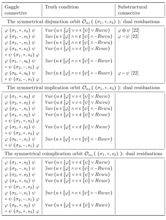
The symmetrical disjunction orbit O–3( (‡1,+, s4) ): dual residuations
Ï(‡1,+, s4) Â ∀uv (u ∈ JÏK ∨ v ∈ JÂK ∨ Ruvw) Ï Â [22] Ï(‡2,−, s5) Â ∃uv (u ∈ JÏK ∧ v ∉ JÂK ∧ −Rwvu) Ï ⌃ Â [22] Ï(‡3,−, s5) Â ∃uv (u ∈ JÏK ∧ v ∉ JÂK ∧ −Rvwu) Ï(‡4,+, s4) Â ∀uv (u ∈ JÏK ∨ v ∈ JÂK ∨ Rvuw) = Â (‡1,+, s4) Ï Ï(‡5,−, s6) Â ∃uv (u ∉ JÏK ∧ v ∈ JÂK ∧ −Rwuv) = Â (‡2,−, s5) Ï Ï(‡6,+, s6) Â ∃uv (u ∉ JÏK ∧ v ∈ JÂK ∧ −Ruwv) Ï ⌥ Â [22] = Â (‡3,−, s5) Ï
The symmetrical implication orbit O–3( (‡1,+, s3) ): dual residuations
Ï(‡1,+, s3) Â ∀uv (u ∉ JÏK ∨ v ∈ JÂK ∨ Ruvw) Ï(‡2,+, s3) Â ∀uv (u ∉ JÏK ∨ v ∈ JÂK ∨ Rwvu) Ï(‡3,−, s1) Â ∃uv (u ∈ JÏK ∧ v ∈ JÂK ∧ −Rvwu) Ï(‡4,+, s2) Â ∀uv (u ∈ JÏK ∨ v ∉ JÂK ∨ Rvuw) = Â (‡1,+, s3) Ï Ï(‡5,+, s2) Â ∀uv (u ∈ JÏK ∨ v ∉ JÂK ∨ Rwuv) = Â (‡2,+, s3) Ï Ï(‡6,−, s1) Â ∃uv (u ∈ JÏK ∧ v ∈ JÂK ∧ −Ruwv) = Â (‡3,−, s1) Ï
The symmetrical coimplication orbit O–3( (‡1,+, s2) ): dual residuations
Ï(‡1,+, s2) Â ∀uv (u ∈ JÏK ∨ v ∉ JÂK ∨ Ruvw) Ï(‡2,−, s1) Â ∃uv (u ∈ JÏK ∧ v ∈ JÂK ∧ −Rwvu) Ï(‡3,+, s3) Â ∀uv (u ∉ JÏK ∨ v ∈ JÂK ∨ Rvwu) Ï(‡4,+, s3) Â ∀uv (u ∉ JÏK ∨ v ∈ JÂK ∨ Rvuw) = Â (‡1,+, s2) Ï Ï(‡5,−, s1) Â ∃uv (u ∈ JÏK ∧ v ∈ JÂK ∧ −Rwuv) = Â (‡2,−, s1) Ï Ï(‡6,+, s2) Â ∀uv (u ∈ JÏK ∨ v ∉ JÂK ∨ Ruwv) = Â (‡3,+, s3) Ï
Gaggle Truth condition Substructural
connective connective
The stroke orbit O–3( (‡1,+, s7) ): Galois connections
Ï(‡1,+, s7)  ∃uv (u ∉ JÏK ∧ v ∉ JÂK ∧ Ruvw) Ï�3 Â[1, 22] Ï(‡2,+, s7)  ∃uv (u ∉ JÏK ∧ v ∉ JÂK ∧ Rwvu) Ï(‡3,+, s7)  ∃uv (u ∉ JÏK ∧ v ∉ JÂK ∧ Rvwu) Ï(‡4,+, s7)  ∃uv (u ∉ JÏK ∧ v ∉ JÂK ∧ Rvuw) =  (‡1,+, s7) Ï Ï(‡5,+, s7)  ∃uv (u ∉ JÏK ∧ v ∉ JÂK ∧ Rwuv) Ï�1 Â[1, 22] =  (‡2,+, s7) Ï Ï(‡6,+, s7)  ∃uv (u ∉ JÏK ∧ v ∉ JÂK ∧ Ruwv) Ï�2 Â[1, 22] =  (‡3,+, s7) Ï
The dagger orbit O–3( (‡1,−, s8) ): Galois connections
Ï(‡1,−, s8) Â ∀uv (u ∉ JÏK ∨ v ∉ JÂK ∨ −Ruvw) Ï ↓3 Â [1, 22] Ï(‡2,−, s8) Â ∀uv (u ∉ JÏK ∨ v ∉ JÂK ∨ −Rwvu) Ï(‡3,−, s8) Â ∀uv (u ∉ JÏK ∨ v ∉ JÂK ∨ −Rvwu) Ï(‡4,−, s8) Â ∀uv (u ∉ JÏK ∨ v ∉ JÂK ∨ −Rvuw) = Â (‡1,−, s8) Ï Ï(‡5,−, s8) Â ∀uv (u ∉ JÏK ∨ v ∉ JÂK ∨ −Rwuv) Ï ↓1 Â [1, 22] = Â (‡2,−, s8) Ï Ï(‡6,−, s8) Â ∀uv (u ∉ JÏK ∨ v ∉ JÂK ∨ −Ruwv) Ï ↓2 Â [1, 22] = Â (‡3,−, s8) Ï
Figure 11: The 2–ary gaggle connectives
Definition 34 (Logic). A logic is a triple L = (L, E, ) where
• L is a language defined as a set of well-formed expressions built from a set of connectives C and a set of atoms P;
• E is a class of pointed models or frames;
• is a satisfaction relation which relates in a compositional manner elements of L to models of E by means of so-called truth conditions.
A L–consecution is an expression of the form Ï Â, Âor Ï , where Ï, Â ∈ L. Our definition of a calculus and of an inference rule is taken from [32].