HAL Id: hal-00945282
https://hal.inria.fr/hal-00945282
Submitted on 24 Mar 2014
HAL is a multi-disciplinary open access
archive for the deposit and dissemination of
sci-entific research documents, whether they are
pub-lished or not. The documents may come from
teaching and research institutions in France or
abroad, or from public or private research centers.
L’archive ouverte pluridisciplinaire HAL, est
destinée au dépôt et à la diffusion de documents
scientifiques de niveau recherche, publiés ou non,
émanant des établissements d’enseignement et de
recherche français ou étrangers, des laboratoires
publics ou privés.
Blind signal decompositions for automatic transcription
of polyphonic music: NMF and K-SVD on the
benchmark
Nancy Bertin, Roland Badeau, Gael Richard
To cite this version:
Nancy Bertin, Roland Badeau, Gael Richard. Blind signal decompositions for automatic transcription
of polyphonic music: NMF and K-SVD on the benchmark. Proc. of IEEE International Conference on
Acoustics, Speech and Signal Processing (ICASSP), 2007, Honolulu, Hawaii, United States. pp.65–68.
�hal-00945282�
BLIND SIGNAL DECOMPOSITIONS FOR AUTOMATIC TRANSCRIPTION OF
POLYPHONIC MUSIC: NMF AND K-SVD ON THE BENCHMARK
Nancy Bertin, Roland Badeau, Ga¨el Richard
GET-T´el´ecom Paris (ENST) - Signal and Image Processing Department
46 rue Barrault - 75634 PARIS Cedex 13, FRANCE
nbertin@enst.fr
ABSTRACT
This paper investigates on the behavior of two blind signal decom-position algorithms, non negative matrix factorization (NMF) and non negative K-SVD (NKSVD), in a polyphonic music transcription task. State-of-the-art transcription systems are based on a frame-by-frame, low-level approach; blind systems could be an alternative to them. Two raw but effective audio-to-MIDI systems are proposed and evaluated. Performances are similar, but in favor of NMF, which is more robust to initialization, choice of the order and computation-nally less costly.
Index Terms— Automatic transcription, polyphonic music, non
negative matrix factorization, K-SVD.
1. INTRODUCTION
Automatic music transcription consists in deriving a symbolic rep-resentation (e.g. a MIDI-like file) of the music from an audio file. Transcribing monodic music is henceforth a well understood prob-lem; but the case of polyphonic music remains a largely open ques-tion.
To address this issue, most of the proposed approaches rely on prior knowledge (e.g. signal models [1] or supervised learning [2, 3]) and/or frame-by-frame low-level analysis. The main weakness of this kind of methods is their low capacity to adapt to signals that do not comply with the model. In order to avoid this drawback, a more recent set of approaches consists in using as few hypotheses as pos-sible about the audio content and trying to separate the notes blindly. Among those techniques we find: sparse coding [4], non-negative matrix factorization (first introduced for image processing in [5]), blind source separation [6] (e.g. independent component analysis), and their variants [7]. They rely on few and weak hypotheses, and show promising results in polyphonic music transcription.
The work presented here investigates further on the efficiency of this kind of approach for a full audio-to-MIDI transcription. In particular, two algorithms are studied: non-negative matrix factor-ization (NMF), proposed in [8], and the non-negative variant of the k-means singular value decompositions algorithm (NKSVD), suc-cessfully applied to image processing in [9]. If both provide an ex-ploitable decomposition, they behave differently with respect to de-sign choices like initialization, length of the analyzed piece or order of the model, which will be discussed here as well.
The two studied algorithms are briefly presented in section 2 and their implementation in an effective transcription system is described in section 3. We then present in section 4 carried on experiments, and their results in section 5. Conclusions and directions for future work are proposed in section 6.
2. BLIND SIGNAL DECOMPOSITIONS
The two algorithms studied in this paper are briefly described be-low since more details can be found in [10] for NMF and in [9] for NKSVD. Although they have their own specificities, both algorithms rely on common hypotheses and principles.
2.1. Common framework
Both algorithms consider the magnitude spectrogram of the data as a linear combination ofr elementary spectra, or atoms, at each time step; determining a decomposition consists in finding the basis of el-ementary atoms, and the decomposition of the data on this basis. The magnitude spectrum is obviously not additive, but this is a relevant approximation in many cases.
Basically, let us consider a time-frequency representationV of a musical excerpt.V is in Rm×n
+ wherem is the number of frequency
bins andn the number of time frames. We search for two matrices W ∈ Rm×r
+ andH ∈ R r×n
+ such that:
V ≈ W H (1)
The approximation is to be understood as a minimization of a “distance” (which has to be defined) between the original V and its reconstructionW H. The specific property exploited here is the non-negativity of all these matrices: they only have zero or positive coefficients. Columns ofW are seen as frequency-domain atoms, and lines ofH are the temporal activities of each of these atoms in the observed signal. At each time framej, the spectrum Vjis thus
expressed as a linear combination of several atoms, the coefficients of the combination being given by thej-th column of H. The re-covered atoms are interpreted as notes and the matrixH as temporal
activities.
2.2. Non-negative matrix factorization (NMF)
In Non-Negative Matrix Factorization, the non-negativity of the ma-trices involved is the only constraint used to process the decomposi-tion. The approximation comes from the constraintr < min(n, m), so that the factorization is also a rank reduction. Considering a long enough music piece, containing a certain number of musical events, the most natural (and, we hope, only) way to represent the signal on a reduced-sized basis should be to have a basis of notes.
The factorization is processed by iterative minimization of a cost function (Frobenius distance or I-divergence, see [10]) and leading to a local minimum; non-negativity is guaranteed by multiplicative update rules at each iteration.
2.3. Non-negative K-SVD (NKSVD)
K-SVD and its non-negative variant, implemented here, is a sparse-coding-like algorithm, developed for image coding and denoising purpose. In typical algorithms, sparse coding (determination of the decomposition of a signal in a given basis) and dictionary design (determination of the basis in which signals will be decomposed) are are often conducted separately. K-SVD was proposed, as a gen-eralization of the k-means algorithm, in order to simultaneously get (and in an unsupervised way) both basis and decomposition.
Sparsity is the property of having few non-zero entries. In music, the intuitive interpretation is that among all possible notes (the 88 keys of the piano for instance), only a few of them can be played si-multaneously by a human musician. It is used in addition to the non-negativity constraint to compute the decomposition. In this model, W is considered as a dictionary, and is generally searched overcom-plete, that isr >> m. Two quantities have to be minimized dur-ing the calculation: the reconstruction error (taken as the Frobenius norm ofV − W H) and the l0
-norm ofH, which conveys the no-tion of sparsity. This is performed iteratively, with two steps at each iteration: pursuit (W being fixed, find the best and sparsest H) and dictionary update (refineW , using singular value decompositions (SVD)).
2.4. Main differences
The main difference between the two algorithms is a matter of “phi-losophy”, in particular as far as the order of the model is concerned. NMF aims at reducing rank, in order to let emerge a meaningful representation; whereas NKSVD, which is in first intention a cod-ing algorithm, aims only at findcod-ing an economical representation (through sparsity), with an overcomplete dictionary. Another dif-ference is related to complexity: NKSVD is much more costly than NMF (about 10 times more CPU time), because of the performed singular value decompositions and because the dictionary is sup-posed to be overcomplete. Eventually, NKSVD allows to control the degree of sparsity of the decomposition; in NMF, sparsity comes as an uncontrolled side effect.
3. THE AUTOMATIC TRANSCRIPTION SYSTEM
The audio-to-MIDI system consists of three steps: processing of a time-frequency representation, its factorization by one of the previ-ously presented algorithms, post-processing of the factors to get a MIDI representation.
3.1. Pre-processing
The short-time Fourier transform of the signal is computed, using a 64 ms Hanning window1 (2822 samples at 44.1 kHz) with a 50% overlap, and its module is taken to get the non-negative matrixV . There are 4096 frequency bins, negative frequencies being then dis-carded, leading to 2048-line matrices.
3.2. Factorization
Non-negative matrix factorization (NMF) and the non-negative vari-ant of the K-SVD (NKSVD) are then performed iteratively onV
1This is obviously a long window, made necessary by frequency
resolu-tion consideraresolu-tions; the choice of the Fourier transform is a well-known limit in this domain, and improvements are bound to find a smarter time-frequency representation, not searched here.
until convergence is reached. Initialization is either random, as pro-posed in the original papers, or set to the spectrum of isolated real piano notes. We implement the most common version of NMF, de-scribed in [10]; in NKSVD, the pursuit stage is performed by Match-ing Pursuit, with a number of retained coefficients set to 10 (i.e. at each frame, at most 10 atoms are active simultaneously).
3.3. Post-processing
The post-processing step consists in interpreting the factorsW and H as respectively, pitched atoms and temporal activities. Each col-umn ofW is considered as a note spectrum. Its pitch is estimated by the maximum of the sum of the log-spectra (rather than the spectral product, in order to avoid numerical errors). Lines ofH associ-ated with atoms of the same pitch are summed. We then determine notes onsets and offsets by thresholding the lines ofH: the atom j is turned on at timek when hjkexceeds a threshold and turned off
when it is below this threshold. The threshold is fixed empirically as the sum of the mean and standard deviation of the line. Velocity was not treated, and arbitrarily set to a constant value. Finally, compo-nents without identified pitch and too short events are discarded. A note event is thus described by a pitch, an onset time and a duration. This post-processing provides a raw, yet useful transcription, for we can listen to the result (by re-synthesis from the MIDI) and com-pare it to a reference. As our purpose was to focus on the previous (factorization) step, we chose coarse methods for this last part, be-ing aware of their weakness and the necessity to refine them in the future.
4. EXPERIMENTS 4.1. Database
Six pieces from the classical piano repertoire, described in [11], are used for tests. They were recorded on a Disklavier mechanically playing the MIDI file in input. Thus, we have a MIDI reference for each test piece, allowing quantitative comparison with the processed transcription. Each piece was then re-synthetized from the MIDI in order to compare the system performances on real and synthetic audio. In addition, the system was also tested on La Campanella by Liszt from the RWC database [12], to evaluate the system in more realistic conditions.
4.2. Parameters
Each piece, in real and synthetized versions, was then systematically analyzed with different values of the model orderr. Initialization was either random or fixed to real piano spectra from the RWC data-base [12].
4.3. Performance evaluation
Music transcription system performance evaluation is a challeng-ing issue, which has not yet reached a consensus in the community. Possible metrics are overviewed in [13]: frame-level metrics (preci-sion/recall and scores agregated from them), note-level metrics, note onset detection error rates. In order to avoid penalizing the whole system because of the coarseness of the back-end (especially tempo-ral) and the slight misalignments in the reference (due to technical constraints of MIDI acquisition), we chose to measure the note onset detection error, with a tolerance of one window (64ms) before and after the reference onset time.
True positive (T P ) is the number of correctly detected notes, false positive (F P ) is the number of wrong notes detected and false negative (F N ) the number of missing notes. Precision rate is the ratioT P/(T P + F P ), recall rate is the ratio T P/(T P + F N ), and
overall accuracyis defined according to [13] as the ratioT P/(T P + F P + F N ).
5. RESULTS 5.1. Preliminary tests
As [8] suggests that notes have to be played alone at least once in the piece in order to get a proper separation, we analyzed this simple example:
Fig. 1. A simple example.
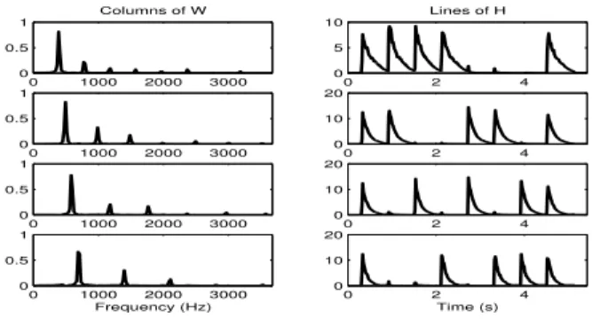
This excerpt was generated by a MIDI synthetizer (with a piano timbre) and analyzed by NMF, with the number of components set to r = 4 (4 different notes are heard). Figure 2 shows the visualization of the result: the 4 columns ofW on the left, the corresponding lines ofH on the right. This way, each left-right pair of graphs shows the frequency content of one component and its temporal occurrences in the analyzed piece.
0 1000 2000 3000 0 0.5 1 Columns of W 0 1000 2000 3000 0 0.5 1 0 1000 2000 3000 0 0.5 1 0 1000 2000 3000 0 0.5 1 Frequency (Hz) 0 2 4 0 5 10 Lines of H 0 2 4 0 10 20 0 2 4 0 10 20 0 2 4 0 10 20 Time (s)
Fig. 2. NMF result of the analysis of Figure 1.
This case is rather ideal: the synthetic sounds make two notes of the same pitch strictly identical, and every possible combination of 2 notes among 4 is played. However, we can also notice that no note is being played alone, yet the algorithm succeeds in separating them. This suggests that NMF can efficiently separate a polyphony even if the notes are never isolated, provided enough various combinations are heard.
5.2. Main experiments: general observations
Though the pieces are rather difficult to transcribe, performed tran-scriptions are good enough to easily recognize the piece when the audio signal is synthetized from the transcribed MIDI file. Most errors are typical of the difficulty of the task: octave-related pitch errors (substitution, insertion or deletion of a note having the same chroma2as the target), note detection errors (notes late or too short,
2Chromais the modulus-12 pitch.
or spurious notes, depending on the choice of the threshold), bad rep-resentation of low-pitched notes, missing notes in chords of 4 notes or more. Performances follow the same trends when analyzing either synthetic or real sounds. This suggests that it would not be unreason-able to test transcription algorithms on databases containing mainly synthetic sounds.
Table 1 shows the mean results of the analysis of the six pieces by NMF and NKSVD, in their synthetic and real versions.r was set to 88.
Table 1. Transcription results (r=88).
Algorithm NMF NKSVD Initialization no yes no yes Precision (%) 52.4 51.4 36.7 44.9 Synth. audio Recall (%) 49.3 54.4 35.9 40.2 Accuracy (%) 34.5 36.1 22.4 25.6 Precision (%) 51.5 45.5 47.0 47.8 Real audio Recall (%) 55.1 56.1 38.1 41.2 Accuracy (%) 36.4 33.6 27.2 29.2 As a reference, for similar analyzed data and identical metrics, accuracies from 30% to 60% are obtained in [13]. Transcription of the Liszt piece showed similar trends, but with lower accuracy, cer-tainly due to the use of the pedal and the fact that the piece is played by a real musician. On this piece, a significative difference was ob-served between NKSVD with and without structured initialization, in favour of the former.
Original and transcription audio examples are available at http://www.enst.fr/˜nbertin/icassp2007.
5.3. Parameters influence
Besides the previous general remarks, we can make some additional observations about the behaviors of the system with respect to dif-ferent parameters and design choices.
5.3.1. Order of the model
Following the original goal of the algorithms, a natural choice for the orderr of the model would be: the theoretical r for NMF (i.e. the number of different pitches in the MIDI reference), and a largely overestimatedr for NKSVD-based transcription. We chose however the same order values for both to keep them comparable. Results are relatively stable with regard to the chosenr, as shown on figure 3. NMF is slightly more sensitive to it, which was rather unexpected.
0 0.5 1 1.5 2 2.5 3 3.5 4 4.5 0 20 40 60 ratio r/rth accuracy NMF NKSVD
Fig. 3. Accuracy w.r.t. the ratio betweenr and the number of
differ-ent pitches in the reference MIDI file (denoted byrth).
At any orderr, we frequently observe that several atoms have the same pitch, corresponding to the most frequent notes appearing in the piece: it is a better strategy for the algorithms to represent
more accurately notes frequently occurring, and the variability be-tween notes of the same pitch increases the need for several atoms to represent each note. This suggests that overestimation of the order is preferable. This is confirmed by figure 3.
5.3.2. Duration of the transcribed piece
Classical, frame-by-frame approaches are indeed not sensitive to the length of the analyzed piece. On the contrary, we expect differ-ent performances of NMF and NKSVD-based transcriptions with respect to this length. Indeed, preliminary tests showed that the variety of chords (notes belonging to different chords) could help a lot to separate notes. We analyzed the first 30 seconds of each test piece separately, and compared the transcription performance with the results we get for the same 30 seconds analyzed within the whole piece. Accuracy is between 5% and 8% higher for the whole piece analysis. It is however difficult to claim without precaution that performance is all the better as the piece is long. The piece must remain somewhat homogeneous along time to benefit from notes re-dundancy.
5.3.3. Initialization
As both algorithms converge to local minima, the initialization of W and H may influence the results. We compared the results of a random initialization ofW vs. a chosen one. Columns of W were then initialized with Fourier magnitude spectra of real piano notes. As we are not supposed to know neither the number of pitches in the piece, nor their values, we fixedr = 88 and initialized W with the 88 notes of the piano.
As shown on table 1, NMF and NKSVD did not show a particu-lar sensitivity to initialization (except that convergence was reached in twice less iterations). Random and determined initialization lead to very similar results, except for NKSVD analysis of the Liszt piece (accuracy is 8% higher with non-random initialization). This obser-vations could be explained by the match or mismatch between ini-tialization spectra and the actual signals.
6. CONCLUSIONS AND FUTURE WORK
The goal of this preliminary work was to assess the potential of two promising approaches for music transcription. The first conclusion is that blind signal decomposition methods may be an alternative to frame-by-frame approach to build efficient transcription systems. Clearly, such methods provide an interesting mid-level representa-tion that could lead, with an efficient post-processing of the decom-position, to a very accurate transcription.
The comparison between NMF and NKSVD does not highlight a clear superiority of one of them upon the other. NMF seems prefer-able for its lower computational cost. NKSVD with initialization was however better on the only real music test piece which suggests further investigation on a larger database.
There are a lot of remaining questions and possible improve-ments. First, an efficient model order estimation method is needed. Second, the problem of complexity and computational cost remains the main handicap of NKSVD. The choice of the pursuit algorithm and of the desired degree of sparsity are other questions to raise. Both methods still need a better back-end (pitch detection in atoms and onset detection in temporal envelopes). For both, the time-frequency representation remains unsatisfactory (because of the well known resolution trade-off of Fourier transform). Eventually, the limitation of the methods to stable spectral profiles (along one note)
is a strong constraint, unrealistic in music (for instance in notes played vibrato). This has to be overtaken, for instance by taking into account the temporal evolution of the note spectrum.
7. ACKNOWLEDGEMENTS
The research leading to this paper was supported by the ACI “Masse de donn´ees” Music Discover, and by the European Commission un-der contract FP6-027026, Knowledge Space of semantic inference fot automatic annotation and retrieval of multimedia content - K-SPACE. The authors also wish to thank Dr. Juan Bello and Dr. Lau-rent Daudet for their sharing audio and MIDI data.
8. REFERENCES
[1] A.P. Klapuri, “Automatic transcription of music,” in
Proceed-ings of the Stockholm Music Acoustics Conference (SMAC), Aug. 2003, vol. II, pp. 587–590.
[2] J. Bello, G. Monti, and M. Sandler, “Techniques for automatic music transcription,” in Proceedings of International
Confer-ence on Music Information Retrieval (ISMIR’00), Oct. 2000. [3] M.D. Plumbley, S.A. Abdallah, J.P. Bello, M.E. Davies,
G. Monti, and M.B. Sandler, “Automatic music transcription and audio source separation,” Cybernetics and Systems, vol. 33, no. 6, pp. 603–627, Sept. 2002.
[4] S.A. Abdallah and M.D. Plumbley, “Unsupervised analysis of polyphonic music using sparse coding,” IEEE Transactions on
Neural Networks, vol. 17, pp. 179–196, Jan. 2006.
[5] D.D. Lee and H.S. Seung, “Learning the parts of objects by non-negative matrix factorization,” Nature, vol. 401, pp. 788– 791, Oct. 1999.
[6] J.F. Cardoso, “Blind signal separation : statistical principles,” in Proc. IEEE. Special issue on blind source separation, 1998, vol. 9, pp. 2009–2025.
[7] M.D. Plumbley, “Algorithms for nonnegative independant component analysis,” IEEE Transactions on Neural Networks, vol. 14, no. 3, pp. 534–543, 2003.
[8] P. Smaragdis and J.C. Brown, “Non-negative matrix factoriza-tion for polyphonic music transcripfactoriza-tion,” in IEEE Workshop
on Applications of Signal Processing to Audio and Acoustics (WASPAA’03), Oct. 2003, pp. 177–180.
[9] M. Aharon, M. Elad, and A. Bruckstein, “K-SVD and its non-negative variant for dictionary design,” in Proceedings of the
SPIE conference wavelets, July 2005, vol. 5914, p. 591411. [10] D.D. Lee and H.S. Seung, “Algorithms for non-negative
ma-trix factorization,” Advances in Neural Information Processing
Systems, vol. 13, pp. 556–562, 2001.
[11] J.P. Bello, L. Daudet, and M.B. Sandler, “Automatic piano transcription using frequency and time-domain information.,”
IEEE Transactions on Speech and Audio Processing, Accepted for publication, 2006.
[12] M. Goto, H. Hashiguchi, T. Nishimura, and R. Oka, “RWC music database: Popular, classical, and jazz music databases,” in Proc. of the 3rd International Conference on Music
Infor-mation Retrieval (ISMIR 2002), October 2002, pp. 287–288. [13] G.E Poliner and D.P.W. Ellis, “A discriminative model for
polyphonic piano transcription,” Eurasip Journal of Applied
Signal Processing (special issue on Music Signal Processing), 2006, to appear.