HAL Id: hal-00285511
https://hal.archives-ouvertes.fr/hal-00285511
Preprint submitted on 6 Jun 2008
HAL is a multi-disciplinary open access archive for the deposit and dissemination of sci-entific research documents, whether they are pub-lished or not. The documents may come from teaching and research institutions in France or
L’archive ouverte pluridisciplinaire HAL, est destinée au dépôt et à la diffusion de documents scientifiques de niveau recherche, publiés ou non, émanant des établissements d’enseignement et de recherche français ou étrangers, des laboratoires
On the Approximability of Comparing Genomes with
Duplicates
Sébastien Angibaud, Guillaume Fertin, Irena Rusu, Annelyse Thevenin,
Stéphane Vialette
To cite this version:
Sébastien Angibaud, Guillaume Fertin, Irena Rusu, Annelyse Thevenin, Stéphane Vialette. On the Approximability of Comparing Genomes with Duplicates. 2008. �hal-00285511�
On the Approximability of Comparing Genomes with Duplicates
S´ebastien Angibaud1, Guillaume Fertin1, Irena Rusu1, Annelyse Th´evenin2, and St´ephane Vialette3
1
Laboratoire d’Informatique de Nantes-Atlantique (LINA), UMR CNRS 6241, Universit´e de Nantes, 2 rue de la Houssini`ere, 44322 Nantes Cedex 3, France
{sebastien.angibaud,guillaume.fertin,irena.rusu}@univ-nantes.fr
2
Laboratoire de Recherche en Informatique (LRI), UMR CNRS 8623, Universit´e Paris-Sud, 91405 Orsay, France [email protected]
3
IGM-LabInfo, UMR CNRS 8049, Universit´e Paris-Est, 5 Bd Descartes 77454 Marne-la-Vall´ee, France [email protected]
Abstract. A central problem in comparative genomics consists in computing a (dis-)similarity measure between two genomes, e.g. in order to construct a phylogenetic tree. A large number of such measures has been proposed in the recent past: number of reversals, number of breakpoints, number of common or conserved intervals, SAD etc. In their initial definitions, all these measures suppose that genomes contain no duplicates. However, we now know that genes can be duplicated within the same genome. One possible approach to overcome this difficulty is to establish a one-to-one correspondence (i.e. a matching) between genes of both genomes, where the correspondence is chosen in order to optimize the studied measure. Then, after a gene relabeling according to this matching and a deletion of the unmatched signed genes, two genomes without duplicates are obtained and the measure can be computed. In this paper, we are interested in three measures (number of breakpoints, number of common intervals and number of conserved intervals) and three models of matching (exemplar, intermediate and maximum matchingmodels). We prove that, for each model and each measure M, computing a matching between two genomes that optimizes M is APX–hard. We show that this result remains true even for two genomes G1 and G2 such that G1 contains no duplicates and no gene of G2 appears more than twice.
Therefore, our results extend those of [7,10,13]. Besides, in order to evaluate the possible existence of approximation algorithms concerning the number of breakpoints, we also study the complexity of the following decision problem: is there an exemplarization (resp. an intermediate matching, a maximum matching) that induces no breakpoint ? In particular, we extend a result of [13] by proving the problem to be NP–complete in the exemplar model for a new class of instances, we note that the problems are equivalent in the intermediate and the exemplar models and we show that the problem is in P in the maximum matching model. Finally, we focus on a fourth measure, closely related to the number of breakpoints: the number of adjacencies, for which we give several constant ratio approximation algorithms in the maximum matching model, in the case where genomes contain the same number of duplications of each gene.
Keywords: genome rearrangements, APX–hardness, duplicate genes, breakpoints, adjacencies, com-mon intervals, conserved intervals, approximation algorithms.
1 Introduction and Preliminaries
In comparative genomics, computing a measure of (dis-)similarity between two genomes is a central problem: such a measure can be used, for instance, to construct phylogenetic trees. The measures defined so far essentially fall into two categories: the first one consists in counting the minimum number of operations needed to transform a genome into another (e.g. the edit distance [21] or the number of reversals [4]). The second one contains (dis-)similarity measures based on the genome structure, such as the number of breakpoints [7], the conserved intervals distance [6], the number of common intervals [10], SAD and MAD [24] etc.
When genomes contain no duplicates, most measures can be computed in polynomial time. However, assuming that genomes contain no duplicates is too limited. Indeed, it has been recently shown that a great number of duplicates exists in some genomes. For example, in [20], authors estimate that 15% of genes are duplicated in the human genome. A possible approach to overcome this difficulty is to specify a one-to-one correspondence (i.e. a matching) between genes of both genomes and to remove the unmatched genes, thus obtaining two genomes with identical gene content and no duplicates. Usually, the above mentioned matching is chosen in order to optimize the studied measure, following the parsimony principle. Three models achieving this correspondence have been proposed : the exemplar model [23], the intermediate model [3] and the maximum matching model [25]. Before defining precisely the measures and models studied in this paper, we need to introduce some notations.
Notations used in the paper. A genome G is represented by a sequence of signed integers (called signed genes). For any genome G, we denote by FG the set of unsigned integers (called genes) that are present in G. For any signed gene g, let −g be the signed gene having the opposite sign and let |g| ∈ FG be the corresponding (unsigned) gene.
Given a genome G without duplicates and two signed genes a, b such that a is located before b, let G[a, b] be the set S ⊆ FG of genes located between genes a and b in G, a and b included. We also note [a, b]Gthe substring (i.e. the sequence of consecutive elements) of G starting at a and finishing at b in G.
Let occ(g, G) be the number of occurrences of a given gene g in a genome G and let occ(G) = max{occ(g, G)|g ∈ FG}. A pair of genomes (G1,G2) is said to be of type (x, y) if occ(G1) = x and occ(G2) = y. A pair of genomes (G1,G2) is said to be balanced if, for each gene g ∈ FG1 ∪ FG2, we have occ(g, G1) = occ(g, G2) (otherwise, (G1,G2) will be said to be unbalanced). Note that a pair (G1, G2) of type (x, x) is not necessary balanced.
Denote by nG the size of genome G, that is the number of signed genes it contains. Let G[p], 1 ≤ p ≤ nG, be the signed gene that occurs at position p on genome G, and let |G[p]| ∈ FG be the corresponding (unsigned) gene. Let NG[p], 1 ≤ p ≤ nG, be the number of occurrences of |G[p]| in the first (p − 1) positions of G.
We define a duo in a genome G as a pair of successive signed genes.Given a duo di = (G[i], G[i + 1]) in a genome G, we note −di the duo equal to (−G[i + 1], −G[i]). Let (d1, d2) be a pair of duos ; (d1, d2) is called a duo match if d1 is a duo of G1, d2 is a duo of G2, and if either d1 = d2 or d1 = −d2.
For example, consider the genome G1 = +1 + 2 + 3 + 4 + 5 − 1 − 2 + 6 − 2. Then, FG= {1, 2, 3, 4, 5, 6}, nG1 = 9, occ(1, G1) = 2, occ(G1) = 3, G1[7] = −2, −G1[7] = +2, |G1[7]| = 2 and NG1[7] = 1. Let G2be the genome G2 = +2 −1 +6 +3 −5 −4 +2 −1 −2. Then the pair (G1, G2) is balanced and is of type (3, 3). Let d1 = (G1[4], G1[5]) be the duo (+4, +5) and d2 be the duo (G2[5], G2[6]). The pair (d1, d2) is a duo match. Now, consider the genome G3= +3−2+6+4−1+5 without duplicates. We have G3[+6, −1] = {1, 4, 6} and [+6, −1]G3 = (+6, +4, −1).
Breakpoints, adjacencies, common and conserved intervals. Let us now define the four measures we will study in this paper. Let G1 and G2 be two genomes without duplicates and with the same gene content, that is FG1 = FG2.
Breakpoint and Adjacency. Let (a, b) be a duo in G1. We say that the duo (a, b) induces a breakpoint of (G1, G2) if neither (a, b) nor (−b, −a) is a duo in G2. Otherwise, we say that (a, b) induces an adjacency of (G1, G2). For example, when G1 = +1 + 2 + 3 + 4 + 5 and G2 = +5 −
4 − 3 + 2 + 1, the duo (2, 3) in G1 induces a breakpoint of (G1, G2) while (3, 4) in G1 induces an adjacency of (G1, G2). We note B(G1, G2) (resp. A(G1, G2)) the number of breakpoints (resp. the number of adjacencies) that exist between G1 and G2.
Common interval. A common interval of (G1, G2) is a substring of G1 such that G2 contains a permutation of this substring (not taking signs into account). For example, consider G1 = +1 + 2 + 3 + 4 + 5 and G2 = +2 − 4 + 3 + 5 + 1. The substring [+3, +5]G1 is a common interval of (G1, G2). Conserved interval. Consider two signed genes a and b of G1 such that a precedes b, where the precedence relation is large in the sense that, possibly, a = b. The substring [a, b]G1 is a conserved interval of (G1, G2) if either (i) a precedes b and G2[a, b] = G1[a, b], or (ii) −b precedes −a and G2[−b, −a] = G1[a, b]. For example, if G1 = +1 + 2 + 3 + 4 + 5 and G2 = −5 − 4 + 3 − 2 + 1, the substring [+2, +5]G1 is a conserved interval of (G1, G2). We note that the notion of conserved interval does not consider the sign of genes. Note also that a conserved interval is actually a common interval, but with additional restrictions on its extremities.
Dealing with duplicates in genomes. When genomes contain duplicates, we cannot directly com-pute the measures defined in the previous paragraph. A solution consists in finding a one-to-one correspondence (i.e. a matching) between duplicated genes of G1 and G2 ; we then use this corre-spondence to rename genes of G1 and G2, and we delete the unmatched signed genes in order to obtain two genomes G′1 and G′2 such that G′2 is a permutation of G′1 ; thus, the measure compu-tation becomes possible. In this paper, we will focus on three models of matching : the exemplar, intermediate and maximum matching models.
– The exemplar model [23]: for each gene g, we keep in the matching M only one occurrence of g in G1 and in G2, and we remove all the other occurrences. Hence, we obtain two genomes GE1 and GE
2 without duplicates. The triplet (GE1, GE2, M) is called an exemplarization of (G1, G2). Note that in this model, M can be inferred from the exemplarized genomes GE
1 and GE2. Thus, in the rest of the paper, any exemplarization (GE
1, GE2, M) of (G1, G2) will be only described by the pair (GE
1, GE2).
– The intermediate model [3]: in this model, for each gene g, we keep in the matching M an arbitrary number kg, 1 ≤ kg ≤ min(occ(g, G1), occ(g, G2)), in order to obtain genomes GI1 and GI
2. We call the triplet (GI1, GI2, M) an intermediate matching of (G1, G2).
– The maximum matching model [25]: in this case, we keep in the matching M the maximum number of signed genes in both genomes. More precisely, we look for a one-to-one correspondence between signed genes of G1 and G2 that matches, for each gene g, exactly min(occ(g, G1), occ(g, G2)) occurrences. After this operation, we delete each unmatched signed gene. The triplet (GM
1 , GM2 , M) obtained by this operation is called a maximum matching of (G1, G2).
Problems studied in this paper. Consider two genomes G1 and G2 with duplicates. Let EComI (resp. IComI, MComI) be the problem which consists in finding an exemplarization (resp. inter-mediate matching, maximum matching) (G′1, G′2, M) of (G1, G2) such that the number of common intervals of (G′1, G′2) is maximized. Moreover, let EConsI (resp. IConsI, MConsI) be the problem which consists in finding an exemplarization (resp. intermediate matching, maximum matching) (G′1, G′2, M) of (G1, G2) such that the number of conserved intervals of (G′1, G′2, M) is maximized. In Section 2, we prove the APX–hardness of EComI and EConsI, even for genomes G1 and G2 such that occ(G1) = 1 and occ(G2) = 2. These results induce the APX–hardness under the other models (i.e., IComI, MComI, IConsI and MConsI are APX–hard). These results extend in particular those of [7,10].
Let EBD (resp. IBD, MBD) be the problem which consists in finding an exemplarization (resp. intermediate matching, maximum matching) (G′1, G′2, M) of (G1, G2) that minimizes the number of breakpoints between G′1 and G′2. In Section 3, we prove the APX–hardness of EBD, even for genomes G1 and G2 such that occ(G1) = 1 and occ(G2) = 2. This result implies that IBD and MBD are also APX–hard, and extends those of [13].
Let ZEBD (resp. ZIBD, ZMBD) be the problem which consists in determining, for two genomes G1and G2, whether there exists an exemplarization (resp. intermediate matching, maximum match-ing) which induces zero breakpoint. In section 4, we study the complexity of ZEBD, ZMBD and ZIBD: in particular, we extend a result of [13] by proving ZEBD to be NP–complete for a new class of instances. We also note that the problems ZEBD and ZIBD are equivalent, and we show that ZMBD is in P.
Finally, in Section 5, we focus on a fourth measure, closely related to the number of breakpoints: the number of adjacencies, for which we give several constant ratio approximation algorithms in the maximum matching model, in the case where genomes are balanced.
2 EComI and EConsI are APX–hard
Consider two genomes G1 and G2 with duplicates, and let EComI (resp. IComI, MComI) be the problem which consists in finding an exemplarization (resp. intermediate matching, maximum matching) (G′
1, G′2, M) of (G1, G2) such that the number of common intervals of (G′1, G′2) is maxi-mized. Moreover, let EConsI (resp. IConsI, MConsI) be the problem which consists in finding an exemplarization (resp. intermediate matching, maximum matching) (G′1, G′2, M) of (G1, G2) such that the number of conserved intervals of (G′
1, G′2, M) is maximized.
EComIand MComI have been proved to be NP–complete even if occ(G1) = 1 and occ(G2) = 2 in [10]. Besides, in [6], Blin and Rizzi have studied the problem of computing a distance built on the number of conserved intervals. This distance differs from the number of conserved intervals we study in this paper, mainly in the sense that (i) it can be applied to two sets of genomes (as opposed to two genomes in our case), and (ii) the distance between two identical genomes of length n is equal to 0 (as opposed to n(n+1)2 in our case). Blin and Rizzi [6] proved that finding the minimum distance is NP–complete, under both the exemplar and maximum matching models. A closer analysis of their proof shows that it can be easily adapted to prove that EConsI and MConsIare NP–complete, even in the case occ(G1) = 1.
We can conclude from the above results that IComI and IConsI are also NP–complete, since when one genome contains no duplicates, exemplar, intermediate and maximum matching models are equivalent.
In this section, we improve the above results by showing that the six problems EComI, IComI, MComI, EConsI, IConsI and MConsI are APX–hard, even when genomes G1 and G2 are such that occ(G1) = 1 and occ(G2) = 2. The main result is Theorem 1, which will be completed by Corollary 1 at the end of the section.
Theorem 1. EComI and EConsI are APX–hard even when genomes G1 and G2 are such that occ(G1) = 1 and occ(G2) = 2.
We prove Theorem 1 by using an L-reduction [22] from the Min-Vertex-Cover problem on cubic graphs, denoted here Min-Vertex-Cover-3. Let G = (V, E) be a cubic graph, i.e. for all v ∈ V, degree(v) = 3. A set of vertices V′ ⊆ V is called a vertex cover of G if for each edge e ∈ E,
there exists a vertex v ∈ V′ such that e is incident to v. The problem Min-Vertex-Cover-3 is defined as follows:
Problem: Min-Vertex-Cover-3 Input: A cubic graph G = (V, E). Solution: A vertex cover V′ of G. Measure: The cardinality of V′.
Min-Vertex-Cover-3 was proved to be APX–complete in [1].
2.1 Reduction
Let G = (V, E) be an instance of Min-Vertex-Cover-3, where G is a cubic graph with V = {v1. . . vn} and E = {e1. . . em}. Consider the transformation R which associates to the graph G two genomes G1 and G2 in the following way, where each gene has a positive sign.
G1 = b1 b2. . . bm x a1 C1 f1 a2 C2 f2. . . an Cn fn y bm+n, bm+n−1. . . bm+1 (1) G2 = y a1 D1 f1 bm+1 a2 D2 f2 bm+2. . . bm+n−1 an Dn fn bm+n x (2) with :
– for each i, 1 ≤ i ≤ n, ai = 6i − 5, fi = 6i
– for each i, 1 ≤ i ≤ n, Ci = (ai+ 1), (ai+ 2), (ai+ 3), (ai+ 4) – for each i, 1 ≤ i ≤ n + m, bi= 6n + i
– x = 7n + m + 1 and y = 7n + m + 2
– for each i, 1 ≤ i ≤ n, Di= (ai+ 3), (bji), (ai+ 1), (bki), (ai+ 4), (bli), (ai+ 2) where eji, eki and eli are the edges which are incident to vi in G, with ji< ki < li.
In the following, genes bi, 1 ≤ i ≤ m, are called markers. There is no duplicated gene in G1 and the markers are the only duplicated genes in G2 ; these genes occur twice in G2. Hence, we have occ(G1) = 1 and occ(G2) = 2.
V2 V1 V3 V4 e2 e5 e1 e6 e4 e3
Fig. 1. The cubic graph G.
To illustrate the reduction, consider the cubic graph G of Figure 1. From G, we construct the following genomes G1 and G2:
b1 z}|{ 25 b2 z}|{ 26 b3 z}|{ 27 b4 z}|{ 28 b5 z}|{ 29 b6 z}|{ 30 x z}|{ 35 1 C1 z }| { 2 3 4 5 6 7 C2 z }| { 8 9 10 11 12 13 C3 z }| { 14 15 16 17 18 19 C4 z }| { 20 21 22 23 24 y z}|{ 36 b10 z}|{ 34 b9 z}|{ 33 b8 z}|{ 32 b7 z}|{ 31 36 |{z} y 1 4 25 2 26 5 27 3 | {z } D1 6 31 |{z} b7 7 10 25 8 28 11 29 9 | {z } D2 12 32 |{z} b8 13 16 26 14 28 17 30 15 | {z } D3 18 33 |{z} b9 19 22 27 20 29 23 30 21 | {z } D4 24 34 |{z} b10 35 |{z} x
2.2 Preliminary results
In order to prove Theorem 1, we first give four intermediate lemmas. In the following, a common interval for the EComI problem or a conserved interval for EConsI is called a robust interval. Besides, a trivial interval will denote either an interval of length one (i.e. a singleton), or the whole genome.
Lemma 1. For any exemplarization (G1, GE2) of (G1, G2), the non trivial robust intervals of (G1, GE2) are necessarily contained in some sequence aiCifi of G1 (1 ≤ i ≤ n).
Proof. We start by proving the lemma for common intervals, and we will then extend it to conserved intervals. First, we prove that, for any exemplarization (G1, GE2) of (G1, G2), each common interval I such that |I| ≥ 2 contains either both of x, y or none of them. This further implies that I covers the whole genome. Suppose there exists a common interval Ix (recall that by definition Ix is on G1) such that |Ix| ≥ 2 and Ix contains x. Let P Ix be the permutation of Ix in GE2. The interval Ix must contain either bm or a1. Let us detail each of the two cases:
(a) If Ixcontains bm, then P Ix contains bmtoo. Notice that there is some i, 1 ≤ i ≤ n, such that bm belongs to Di in GE
2. Then P Ix contains all genes between Di and x in GE2. Thus P Ix contains bm+n. Consequently, Ix contains bm+nand it also contains y.
(b) If Ix contains a1, then P Ix contains a1 too. Then P Ix contains all genes between a1 and x. Thus P Ix contains bm+n. Hence, Ix contains bm+n and then it also contains y.
Now, suppose that Iy is a common interval such that |Iy| ≥ 2 and Iy contains y. Let P Iy be the permutation of Iy on GE
2. The interval Iy must contain either bm+nor fn. Let us detail each of the two cases:
(a) If Iy contains bm+n, then P Iy contains bm+n too. Thus P Iy contains all genes between bm+n and y. Hence P Iy contains all the sequences Di, 1 ≤ i ≤ n. In particular, P Iy contains all the markers and consequently Iy must contain x.
(b) If Iy contains fn, then P Iy contains fn too. Then P Iy contains all genes between fn and y. In particular, P Iy contains bm+n−1 and then Iy contains bm+n−1 too. Hence, Iy also contains bm+n, similarly to the previous case. Thus Iy contains x.
We conclude that each non singleton common interval containing either x or y necessarily contains both x and y. Therefore, and by construction of G2, there is only one such interval, that is G1 itself. Hence, any non trivial common interval is necessarily, in G1, either strictly on the left of x, or between x and y, or strictly on the right of y. Let us analyze these different cases:
– Let I be a non trivial common interval situated strictly on the left of x in G1. Thus I is a sequence of at least two consecutive markers. Since in any exemplarization (G1, GE2) of (G1, G2), every marker in GE
2 has neighboring genes which are not markers, this contradicts the fact that I is a common interval.
– Let I be a non trivial common interval situated strictly on the right of y in G1. Then I is a substring of bm+n, . . . , bm+1 containing at least two genes. In any exemplarization (G1, GE2) of (G1, G2), for each pair (bm+i, bm+i+1) of GE2, with 1 ≤ i < n, we have ai+1∈ GE2[bm+i, bm+i+1]. This contradicts the fact that I is strictly on the right of y in G1.
– Let I be a non trivial common interval lying between x and y in G1. For any exemplarization (G1, GE2) of (G1, G2), a common interval cannot contain, in G1, both fi and ai+1 for some i, 1 ≤ i ≤ n − 1 (since bm+i is situated between fi and ai+1 in GE
2 and on the right of x in G1). Hence, a non trivial common interval of (G1, GE2) is included in some sequence aiCifi in G1, 1 ≤ i ≤ n.
This proves the lemma for common intervals. By definition, any conserved interval is necessarily a common interval. So, a non trivial conserved interval of (G1, GE2) is included in some sequence aiCifi in G1, 1 ≤ i ≤ n. The lemma is proved. ⊓⊔ Lemma 2. Let (G1, GE2) be an exemplarization of (G1, G2) and i ∈ [1 . . . n]. Let ∆i be a substring of [ai + 3, ai + 2]GE
2 that does not contain any marker. If |∆i| ∈ {2, 3}, then there is no robust interval I of (G1, GE2) such that ∆i is a permutation of I.
Proof. First, we prove that there is no permutation I of ∆i such that I is a common interval of (G1, GE2). Next, we show that there is no permutation I of ∆isuch that I is a conserved interval. By Lemma 1, we know that a non trivial common interval of (G1, GE2) is a substring of some sequence aiCifi, 1 ≤ i ≤ n. This substring contains only consecutive integers. Therefore, if there exists a permutation I of ∆i such that I is a common interval of (G1, GE2), then ∆i must be a permutation of consecutive integers. If |∆i| = 2, we have ∆i= (p, q) where p and q are not consecutive integers and if |∆i| = 3, then we have ∆i = (ai+ 3, ai+ 1, ai+ 4) or ∆i = (ai+ 1, ai+ 4, ai+ 2). In these three cases, ∆i is not a permutation of consecutive integers. Hence, there is no permutation I of ∆i such that I is a common interval of (G1, GE2). Moreover, any conserved interval is also a common interval. Thus, there is no permutation I of ∆i such that I is a conserved interval of (G1, GE2). ⊓⊔ For more clarity, let us now introduce some notations. Given a graph G = (V, E), let V C = {vi1, vi2. . . vik} be a vertex cover of G. Let R(G) = (G1, G2) be the pair of genomes defined by the construction described in (1) and (2). Now, let F be the function which associates to V C, G1 and G2 an exemplarization F (V C) of (G1, G2) as follows. In G2, all the markers are removed from the sequences Di for all i 6= i1, i2. . . ik. Next, for each marker which is still present twice, one of its occurrences is arbitrarily removed. Since in G2 only markers are duplicated, we conclude that F (V C) is an exemplarization of (G1, G2).
Given a cubic graph G and genomes G1 and G2 obtained by the transformation R(G), let us define the function S which associates to an exemplarization (G1, GE2) of (G1, G2) the vertex cover V C of G defined as follows: V C = {vi|1 ≤ i ≤ n ∧ ∃j ∈ {1 . . . m}, bj ∈ GE
2[ai, fi]}. In other words, we keep in V C the vertices vi of G for which there exists some gene bj such that bj is in GE2[ai, fi]. We now prove that V C is a vertex cover. Consider an edge ep of G. By construction of G1 and G2, there exists some i, 1 ≤ i ≤ n, such that gene bp is located between ai and fi in GE
2. The presence of gene bp between ai and fi implies that vertex vi belongs to V C. We conclude that each edge is incident to at least one vertex of V C.
Let W be the function defined on {EConsI, EComI} by W (pb) = 1 if pb = EConsI and W (pb) = 4 if pb = EComI. Let optP(A) be the optimum result of an instance A for an optimization problem pb, pb ∈ {EcomI, EConsI, Min-Vertex-Cover-3}.
We now define the function T whose arguments are a problem pb ∈ {EConsI, EComI} and a cubic graph G. Let R(G) = (G1, GE2) as usual. Then T (pb, G) is defined as the number of robust trivial intervals of (G1, GE2) with respect to pb. Let n and m be respectively the number of vertices
and the number of edges of G. We have T (EConsI, G) = 7n+m+2 and T (EComI, G) = 7n+m+3. Indeed, for EComI, there are 7n + m + 2 singletons and we also need to consider the whole genome. Lemma 3. Let pb ∈ {EcomI, EConsI}. Let G be a cubic graph and R(G) = (G1, G2). Let (G1, GE2) be an exemplarization of (G1, G2) and let i, 1 ≤ i ≤ n. Then only two cases can oc-cur with respect to Di.
1. Either in GE2, all the markers from Di were removed, and in this case, there are exactly W (pb) non trivial robust intervals involving Di.
2. Or in GE2, at least one marker was kept in Di, and in this case, there is no non trivial robust interval involving Di.
Proof. We first prove the lemma for the EComI problem and then we extend it to EConsI. Lemma 1 implies that each non trivial common interval I of (G1, GE2) is contained in some substring of aiCifi, 1 ≤ i ≤ n. So, the permutation of I on GE2 is contained in a substring of aiDifi, 1 ≤ i ≤ n. Consider i, 1 ≤ i ≤ n, and suppose that all the markers from Di are removed on GE2. Thus, aiCifi, Ci, aiCiand Cifiare common intervals of (G1, GE2). Let us now show that there is no other non trivial common interval involving Di. Let ∆i be a substring of [ai + 3, ai + 2]GE
2 such that |∆i| ∈ {2, 3}. By Lemma 2, we know that ∆iis not a common interval. The remaining intervals are (ai, ai+ 3), (ai, ai+ 3, ai+ 1), (ai, ai+ 3, ai+ 1, ai+ 4), (ai+ 1, ai+ 4, ai+ 2, fi), (ai+ 4, ai+ 2, fi) and (ai+ 2, fi). By construction, none of them can be a common interval, because none of them is a permutation of consecutive integers. Hence, there are only four non trivial common intervals involving Di in GE
2. Among these four common intervals, only aiCifi is a conserved interval too. In the end, if all the markers are removed from Di, there are exactly four non trivial common intervals and one non trivial conserved interval involving Di. So, given a problem pb ∈ {EcomI, EconsI}, there are exactly W (pb) non trivial robust intervals involving Di.
Now, suppose that at least one marker of Di is kept in GE
2. Lemma 1 shows that each non trivial common interval I of (G1, GE2) is contained in some substring of aiCifi, 1 ≤ i ≤ n. Since no marker is present in a sequence aiCifi, we deduce that there does not exist any trivial common interval containing a marker. So, a non trivial common interval involving Di only must contain a substring ∆i of [ai+ 3, ai+ 2]GE
2 such that ∆i contains no marker. Since no marker is an extremity of [ai+ 3, ai+ 2]GE
2, we have |∆i| ≤ 3. By Lemma 2, we know that ∆i is not a common interval. The remaining intervals to be considered are the intervals ai∆iand ∆ifi. By construction of aiCifi, these intervals are not common intervals (the absence of gene ai+ 2 for ai∆i and of gene ai+ 3 for ∆ifi implies that these intervals are not a permutation of consecutive integers). Hence, these intervals cannot be conserved intervals either. ⊓⊔ Lemma 4. Let pb ∈ {EcomI, EConsI}. Let G = (V, E) be a cubic graph with V = {v1. . . vn} and E = {e1. . . em} and let G1, G2 be the two genomes obtained by R(G).
1. Let V C be a vertex cover of G and denote k = |V C|. Then the exemplarization F (V C) of (G1, G2) has at least N = n W (pb) + T (pb, G) − W (pb) · k robust intervals.
2. Let (G1, GE2) be an exemplarization of (G1, G2) and let V C′ be the vertex cover of G obtained by S(G1, GE2). Then |V C′| = W(pb)·n+T (pb,G)−NW(pb) , where N is the number of robust intervals of (G1, GE2).
Proof. 1. Let pb ∈ {EcomI, EConsI}. Let G be a cubic graph and let G1 and G2 be the two genomes obtained by R(G). Let V C be a vertex cover of G and denote k = |V C|. Let (G1, GE2) be the
exemplarization of (G1, G2) obtained by F (V C). By construction, we have at least (n−k) substrings Di in GE2 for which all the markers are removed. By Lemma 3, we know that each of these substrings implies the existence of W (pb) non trivial robust intervals. So, we have at least W (pb)(n − k) non trivial robust intervals. Moreover, by definition of T (pb, G), the number of trivial robust intervals of (G1, GE2) is exactly T (pb, G). Thus, we have at least N = W (pb) · n + T (pb, G) − W (pb) · k robust intervals of (G1, GE2).
2. Let (G1, GE2) be an exemplarization of (G1, G2) and let n − j be the number of sequences Di, 1 ≤ i ≤ n, for which all markers have been deleted in GE
2. Then, by Lemmas 1 and 3, the number of robust intervals of (G1, GE2) is equal to N = W (pb) · n + T (pb, G) − W (pb) · j. Let V C′ be the vertex cover obtained by S(G1, GE2). Each marker has one occurrence in GE2 and these occurrences lie in j sequences Di. So, by definition of S, we conclude that |V C′| = j = W(pb)·n+T (pb,G)−NW(pb) . ⊓⊔
2.3 Main result
Let us first define the notion of L-reduction [22]: let A and B be two optimization problems and cA, cB be respectively their cost functions. An L-reduction from problem A to problem B is a pair of polynomial-time computable functions R and S with the following properties:
(a) If x is an instance of A, then R(x) is an instance of B ;
(b) If x is an instance of A and y is a solution of R(x), then S(y) is a solution of A ;
(c) If x is an instance of A and R(x) is its corresponding instance of B, then there is some positive constant α such that optB(R(x)) ≤ α.optA(x) ;
(d) If s is a solution of R(x), then there is some positive constant β such that |optA(x) − cA(S(s))| ≤ β|optB(R(x)) − cB(s)|.
We prove Theorem 1 by showing that the pair (R, S) defined previously is an L-reduction from Min-Vertex-Cover-3 to EConsI and from Min-Vertex-Cover-3 to EComI. First note that properties (a) and (b) are obviously satisfied by R and S.
Consider pb ∈ {EcomI, EConsI}. Let G = (V, E) be a cubic graph with n vertices and m edges. We now prove properties (c) and (d). Consider the genomes G1 and G2 obtained by R(G). For sake of clarity, we abbreviate here and in the following optMin-Vertex-Cover-3to optMin-VC. First, we need to prove that there exists α ≥ 0 such that optpb(G1, G2) ≤ α.optMin-Vertex-Cover-3(G).
Since G is cubic, we have the following properties:
n ≥ 4 (3) m = 1 2 n X i=1 degree(vi) = 3n 2 (4) optMin-VC(G) ≥ m 3 = n 2 (5)
To explain property (5), remark that, in a cubic graph G with n vertices and m edges, each vertex covers three edges. Thus, a set of k vertices covers at most 3k edges. Hence, any vertex cover of G must contain at least m3 vertices.
By Lemma 3, we know that sequences of the form aiCifi, 1 ≤ i ≤ n, contain either zero or W (pb) non trivial robust intervals. By Lemma 1, there are no other non trivial robust intervals. So, we have the following inequality:
optpb(G1, G2) ≤ T (pb, G) | {z } trivial robust intervals
+W (pb) · n If pb = EComI, we have: optEComI(G1, G2) ≤ 7n + m + 3 + 4n optEComI(G1, G2) ≤ 27n 2 by (3) and (4) (6)
And if pb = EConsI, we have :
optEConsI(G1, G2) ≤ 7n + m + 2 + n optEConsI(G1, G2) ≤ 21n
2 by (3) and (4) (7)
Altogether, by (5), (6) and (7), we prove property (c) with α = 27.
Now, let us prove property (d). Let V C = {vi1, vi2. . . viP} be a minimum vertex cover of G. Then P = optMin-VC(G). Let G1 and G2 be the genomes obtained by R(G). Let (G1, GE2) be an exemplarization of (G1, G2) and let k′ be the number of robust intervals of (G1, GE2). Finally, let V C′ be the vertex cover of G such that V C′ = S(G
1, GE2). We need to find a positive constant β such that |P − |V C′|| ≤ β|optpb(G1, G2) − k′|.
For pb ∈ {EcomI, EConsI}, let Npbbe the number of robust intervals between the two genomes obtained by F (V C). By the first property of Lemma 4, we have
optpb(G1, G2) ≥ Npb≥ W (pb) · n + T (pb, G) − W (pb) · P
So, it is sufficient to prove that there exists some β ≥ 0 such that |P − |V C′|| ≤ β|W (pb) · n + T (pb, G)−W (pb)·P −k′|. By the second property of Lemma 4, we have |V C′| = W(pb)·n+T (pb,G)−k′
W(pb) . Since P ≤ |V C′|, we have |P − |V C′|| = |V C′| − P = W(pb)·n+T (pb,G)−k′
W(pb) − P = W(pb)1 (W (pb) · n + T (pb, G) − W (pb) · P − k′).
So β = 1 is sufficient in both cases, since W (EComI) = 4 and W (EConsI) = 1, which implies 1
W(pb) ≤ 1.
Altogether, we then have |optMin-VC(G) − |V C′|| ≤ 1 · |opt
pb(G1, G2) − k′|.
We proved that the reduction (R, S) is an L-reduction. This implies that for two genomes G1 and G2, both problems EConsI and EComI are APX–hard even if occ(G1) = 1 and occ(G2) = 2.
Theorem 1 is proved. ⊓⊔
We extend in Corollary 1 our results for the intermediate and maximum matching models.
Corollary 1. IComI, MComI, IConsI and MConsI are APX–hard even when genomes G1 and G2 are such that occ(G1) = 1 and occ(G2) = 2.
Proof. The intermediate and maximum matching models are identical to the exemplar model when one of the two genomes contains no duplicates. Hence, the APX–hardness result for EComI (resp. EConsI) also holds for IComI and MComI (resp. IConsI and MConsI). ⊓⊔
3 EBD is APX–hard
Consider two genomes G1and G2 with duplicates, and let EBD (resp. IBD, MBD) be the problem which consists in finding an exemplarization (resp. intermediate matching, maximum matching) (G′
1, G′2, M) of (G1, G2)that minimizes the number of breakpoints between G′1 and G′2.
EBD has been proved to be NP–complete even if occ(G1) = 1 and occ(G2) = 2 [7]. Some inapproximability results also exist: in particular, it has been proved in [13] that, in the general case, EBD cannot be approximated within a factor c log n, where c > 0 is a constant, and cannot be approximated within a factor 1.36 when occ(G1) = occ(G2) = 2. Moreover, for two balanced genomes G1 and G2 such that k = occ(G1) = occ(G2), several approximation algorithms for MBD are given. These approximation algorithms admit respectively a ratio of 1.1037 when k = 2 [17], 4 when k = 3 [17] and 4k in the general case [19]. We can conclude from the above results that IBD and MBD problems are also NP–complete, since when one genome contains no duplicates, exemplar, intermediate and maximum matching models are equivalent.
In this section, we improve the above results by showing that the three problems EBD, IBD and MBDare APX–hard, even when genomes G1 and G2 are such that occ(G1) = 1 and occ(G2) = 2. The main result is Theorem 2 below, which will be completed by Corollary 2 at the end of the section.
Theorem 2. EBD is APX–hard even when genomes G1 and G2 are such that occ(G1) = 1 and occ(G2) = 2.
To prove Theorem 2, we use an L-Reduction from Min-Vertex-Cover-3 to EBD. Let G = (V, E) be a cubic graph with V = {v1. . . vn} and E = {e1. . . em}. For each i, 1 ≤ i ≤ n, let efi, egi and ehi be the three edges which are incident to vi in G with fi < gi< hi. Let R′ be the polynomial transformation which associates to G the following genomes G1 and G2, where each gene has a positive sign:
G1= a0 a1 b1 a2 b2. . . an bn c1 d1 c2 d2. . . cm dm cm+1
G2= a0 an dfn dgn dhn bn. . . a2 df2 dg2 dh2 b2 a1 df1 dg1 dh1 b1 c1 c2. . . cm cm+1 with :
– a0 = 0, and for each i, 1 ≤ i ≤ n, ai = i and bi = n + i
– cm+1= 2n + m + 1, and for each i, 1 ≤ i ≤ m, ci = 2n + i and di= 2n + m + 1 + i
We remark that there is no duplication in G1, so occ(G1) = 1. In G2, only the genes di, 1 ≤ i ≤ m, are duplicated and occur twice. Thus occ(G2) = 2.
Let G be a cubic graph and V C be a vertex cover of G. Let G1and G2 be the genomes obtained by R′(G). We define F′ to be the polynomial transformation which associates to V C, G1 and G2 the exemplarization F′(V C) = (G
1, GE2) of (G1, G2) as follows. For each i such that vi ∈ V C, we/ remove from G2 the genes dfi, dgi and dhi. Then, for each j, 1 ≤ j ≤ m such that dj still has two occurrences in G2, we arbitrarily remove one of these occurrences in order to obtain the genome GE
2. Hence, (G1, GE2) is an exemplarization of (G1, G2).
Given a cubic graph G, we construct G1 and G2 by the transformation R′(G). Given an ex-emplarization (G1, GE2) of (G1, G2), let S′ be the polynomial transformation which associates to (G1, GE2) the set V C = {vi|1 ≤ i ≤ n, ai and bi are not consecutive in GE2}. We claim that V C is a vertex cover of G. Indeed, let ep, 1 ≤ p ≤ m, be an edge of G. Genome GE
2 contains one occurrence of gene dp since GE
that dp is in GE2[ai, bi] and such that ep is incident to vi. The presence of dp in GE2[ai, bi] implies that vertex vi belongs to V C. We can conclude that each edge of G is incident to at least one vertex of V C.
Lemmas 5 and 6 below are used to prove that (R′, S′) is an L-Reduction from the Min-Vertex-Cover-3 problem to the EBD problem. Let G = (V, E) be a cubic graph with V = {v1, v2. . . vn} and E = {e1, e2. . . em} and let us construct (G1, G2) by the transformation R′(G).
Lemma 5. Let V C be a vertex cover of G and (G1, GE2) the exemplarization given by F′(V C). Then |V C| = k ⇒ B(G1, GE2) ≤ n + 2m + k + 1, where B(G1, GE2) is the number of breakpoints between G1 and GE2.
Proof. Suppose |V C| = k. Let us list the breakpoints between genomes G1 and GE2 obtained by F′(V C). The pairs (bi, ai+1), 1 ≤ i ≤ n − 1, and (bn, c1) induce one breakpoint each. For all i, 1 ≤ i ≤ m, each pair of the form (ci, di) (resp. (di, ci+1)) induces one breakpoint. For all i, 1 ≤ i ≤ n, such that vi ∈ V C, (ai, bi) induces at most one breakpoint. Finally, the pair (a0, a1) induces one breakpoint. Thus there are at most n + 2m + k + 1 breakpoints of (G1, GE2). ⊓⊔ Lemma 6. Let (G1, GE2) be an exemplarization of (G1, G2) and V C′ be the vertex cover of G obtained by S′(G1, GE2). We have B(G1, GE2) = k′⇒ |V C′| = k′− n − 2m − 1.
Proof. Let (G1, GE2) be an exemplarization of (G1, G2) and V C′ be the vertex cover obtained by S′(G
1, GE2). Suppose B(G1, GE2) = k′. For any exemplarization (G1, GE2) of (G1, G2), the following breakpoints always occur: the pair (a0, a1) ; for each i, 1 ≤ i ≤ m, each pair (ci, di) and (di, ci+1) ; for each i, 1 ≤ i ≤ n − 1, the pair (bi, ai+1) ; the pair (bn, c1). Thus, we have at least n + 2m + 1 breakpoints. The other possible breakpoints are induced by pairs of the form of (ai, bi). Since we have B(G1, GE2) = k′, there are exactly k′− n − 2m − 1 such breakpoints. By construction of V C′, the cardinality of V C′ is equal to the number of breakpoints induced by pairs of the form (ai, bi). So, we have: |V C′| = k′− n − 2m − 1. ⊓⊔ To prove that (R′, S′) is an reduction, we first notice that properties (a) and (b) of an L-reduction are trivially verified. The next lemma proves property (c).
Lemma 7. The inequality optEBD(G1, G2) ≤ 12 · optMin-VC(G) holds.
Proof. For a cubic graph G with n vertices and m edges, we have 2m = 3n (see (4)) and optMin-VC(G) ≥ n
2(see (5)). By construction of the genomes G1 and G2, any exemplarization of (G1, G2) contains 2n+2m+2 genes in each genome. Thus, we have optEBD(G1, G2) ≤ 2n+2m+2 ≤ 6n (n ≥ 4 in a cubic graph). Hence, we conclude that optEBD(G1, G2) ≤ 12 · optMin-VC(G). ⊓⊔
Now, we prove property (d) of our L-reduction.
Lemma 8. Let (G1, GE2) be an exemplarization of (G1, G2) and let V C′ be the vertex cover of G obtained by S′(G1, GE2). Then, we have |optMin-VC(G) − |V C′|| ≤ |optEBD(G1, G2) − B(G1, GE2)| Proof. Let (G1, GE2) be an exemplarization of (G1, G2) and V C′ be the vertex cover of G obtained by S′(G
1, GE2). Let V C be a vertex cover of G such that |V C| = optMin-VC(G).
We know that optMin-VC(G) ≤ |V C′| and optEBD(G1, G2) ≤ B(G1, GE2). So, it is sufficient to prove |V C′| − optMin-VC(G) ≤ B(G1, GE2) − optEBD(G1, G2).
By Lemma 5, we have B(F′(V C)) ≤ n + 2m + 1 + optMin-VC, which implies optEBD(G
1, G2) ≤ B(F′(V C)) ≤ n + 2m + 1 + optMin-VC. Then
B(G1, GE2) − optEBD(G1, G2) ≥ B(G1, GE2) − n − 2m − 1 − optMin-VC(G) (8)
By Lemma 6, we have: |V C′| = B(G1, GE2) − n − 2m − 1 which implies
|V C′| − optMin-VC(G) = B(G1, GE
2) − n − 2m − 1 − optMin-VC(G) (9) Finally, by (8) and (9), we get |V C′| − optMin-VC≤ B(G1, GE
2) − optEBD(G1, G2). ⊓⊔ Lemmas 7 and 8 prove that the pair (R′, S′) is an L-reduction from Min-Vertex-Cover-3 to EBD. Hence, EBD is APX–hard even if occ(G1) = 1 and occ(G2) = 2, and Theorem 2 is proved. We extend in Corollary 2 our results for the intermediate and maximum matching models.
Corollary 2. The IBD and MBD problems are APX–hard even when genomes G1 and G2 are such that occ(G1) = 1 and occ(G2) = 2.
Proof. The intermediate and maximum matching models are identical to the exemplar model when one of the two genomes contains no duplicates. Hence, the APX–hardness result for EBD also
holds for IBD and MBD. ⊓⊔
4 Zero breakpoint distance
This section is devoted to zero breakpoint distance recognition issues. Indeed, in [13], the authors showed that deciding whether the exemplar breakpoint distance between any two genomes is zero or not is NP–complete even when no gene occurs more than three times in both genomes, i.e., instances of type (3, 3). This important result implies that the exemplar breakpoint distance problem does not admit any approximation in polynomial-time, unless P = NP. Following this line of research, we first complement the result of [13] by proving that deciding whether the exemplar breakpoint distance between any two genomes is zero or not is NP–complete, even when no gene is duplicated more than twice in one of the genomes (the maximum number of duplications is however unbounded in the other genome). This result is next extended to the intermediate matching model and we give a practical - but exponential - algorithm for deciding whether the exemplar breakpoint distance between any two genomes is zero or not in case no gene occurs more than twice in both genomes (a problem whose complexity, P versus NP–complete, remains open). Finally, we show that deciding whether the maximum matching breakpoint distance between any two genomes is zero or not is polynomial-time solvable and hence that such negative approximation results (the ones we obtained for the exemplar and intermediate models) do no propagate to the maximum matching model.
The following easy observation will prove extremely useful in the sequel of the present section.
Observation 3 Let G1 and G2 be two genomes. If the exemplar breakpoint distance between G1 and G2 is zero, then there exists an exemplarization (GE1, GE2) of (G1, G2) such that (1) GE1 = GE2, or (2) −(GE
1)r = GE2, where −(GE1)r is the signed reversal of genome G1. The same observation can be made for the intermediate and maximum matching models.
4.1 Zero exemplar breakpoint distance
The zero exemplar breakpoint distance (ZEBD) problem is formally defined as follows. Problem: ZEBD
Input: Two genomes G1 and G2.
Question: Is the exemplar breakpoint distance between G1 and G2 equal to zero?
Aiming at precisely defining the inapproximability landscape of computing the exemplar break-point distance between two genomes, we complement the result of [13], who showed ZEBD to be NP–complete even for instances of type (3, 3), by the following theorem.
Theorem 4. ZEBD is NP–complete even if no gene occurs more than twice in G1.
Proof. Membership of ZEBD to NP is immediate. The reduction we use to prove hardness is from Min-Vertex-Cover[16]. Let an arbitrary instance of Min-Vertex-Cover be given by a graph G = (V, E) and a positive integer k. Write V = {v1, v2. . . vn} and E = {e1, e2. . . em}. In the rest of the proof, elements of V (resp. E) will be seen either as vertices (resp. edges) or genes, depending on the context. The corresponding instance (G1, G2) of ZEBD is defined as follows:
G1 = v1 X1 v2 X2. . . vn Xn G2 = Y [1] Y [2] . . . Y [k] YV.
For each i = 1, 2, . . . , n, Xi is defined to be Xi = ei1 ei2 . . . eij, where ei1, ei2, . . . , eij, i1 < i2 < . . . < ij, are the edges incident to vertex vi. The strings Y [i], 1 ≤ i ≤ k, are all equal and are defined by Y [i] = YV YE where YV = v1 v2 . . . vn and YE = e1 e2 . . . em.
Notice that no gene occurs more than twice in G1 (actually genes vi occur once and genes ei occur twice). However, the number of occurrences of each gene in G2 is upper bounded by k + 1. Furthermore, all genes have positive sign, and hence according to Observation 3 we only need to consider exemplarizations (GE
1, GE2) of (G1, G2) such that GE1 = GE2.
It is immediate to check that our construction can be carried out in polynomial-time. We now claim that there exists a vertex cover of size k in G iff the exemplar breakpoint distance between G1 and G2 is zero.
Suppose first that there exists a vertex cover V′⊆ V of size k in G. Write V′ = {vi1, vi2, . . . , vi k}, i1 < i2 < . . . < ik. For convenience, we also define i0 to be 0. From V′ we construct an exemplar-ization (GE
1, GE2) as follows. We obtain GE1 from G1 by a two step procedure. First we delete in G1 all strings Xi such that vi ∈ V/ ′. Second, for each 1 ≤ j ≤ m, if gene ej still occurs twice, we delete its second occurrence (this second step is concerned with edges connecting two vertices in V′). We now turn to GE
2. For 1 ≤ j ≤ k, we consider the string Y [j] = YV YE that we process as follows: (1) we delete in YV all genes but vij and those genes vℓ ∈ V/ ′ such that ij−1 < ℓ < ij, and (2) we delete in YE all genes but those eℓ that are not incident to vij or incident to vij and some smaller vertex in V′ (i.e., eℓ = {vij′, vij} for some j′ < j). Finally, we delete in the trailing string YV = v1 v2 . . . vn all genes but those vℓ ( /∈ V′) such that ik < ℓ. Since V′ is a vertex cover in G, then it follows that each gene occurs once in the obtained genomes, i.e., (GE
1, GE2) is indeed an exemplarization of (G1, G2). It is now easily seen that GE1 = GE2, and hence that the exemplar breakpoint distance between G1 and G2 is zero.
Conversely, suppose that the exemplar breakpoint distance between G1 and G2 is zero. Since all genes have a positive sign, then it follows that there exists an exemplarization (GE1, GE2) of (G1, G2) such that GE
1 = GE2. Exemplarization GE2 can be written as
GE2 = YV[1] YE[1] YV[2] YE[2] . . . YV[k] YE[k] YV[k + 1]
where, YV[i], 1 ≤ i ≤ k + 1, is a string on V and YE[i], 1 ≤ i ≤ k, is a string on E, V and E being viewed as alphabets. Now, define V′⊆ V as follows: vi∈ V′ iff gene vi occurs in some YV[j], 1 ≤ j ≤ k, as the last gene. By construction, |V′| ≤ k (we may indeed have |V′| < k if some YV[j], 1 ≤ j ≤ k, denotes the empty string). We now observe that, since no gene vi is duplicated in G1, all genes eℓ that occur between some gene vi ∈ V′ and some gene vj ∈ V in GE
2 should match genes in string Xi in G1. Then it follows that V′ is a vertex cover of size at most k in G. ⊓⊔ The complexity of ZEBD remains open in case no gene occurs more than twice in G1 and more than a constant times in G2, i.e., instances of type (2, c) for some c = O(1) ; recall here that ZEBD is NP–complete if no gene occurs more than three times in G1 or in G2 (instances of type (3, 3), [13]). In particular, the complexity of ZEBD for instances of type (2, 2) is open. However, we propose here a practical - but exponential - algorithm for ZEBD for instances of type (2, 2), which is well-suited in case the number of genes that occur twice both in G1 and in G2 is relatively small.
Proposition 1. ZEBD for instances of type (2, 2) (no gene occurs more than twice in G1 and in G2) is solvable in O∗(1.61822k) time, where k is upper-bounded by the number of genes that occur exactly twice in G1 and in G2.
Proof. According to Observation 3, for any instance (G1, G2), we only need to focus on exemplar-izations (GE
1, GE2) such that GE1 = GE2 or −(G1E)r = GE2, where −(GE1)r is the signed reversal of GE
1. Let us first consider the case GE1 = GE2 (the case −(GE1)r = GE2 is identical up to a signed reversal and will thereby be briefly discussed at the end of the proof).
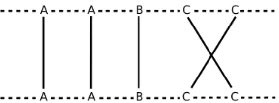
Let (G1, G2) be an instance of type (2, 2) of ZEBD. Our algorithm is by transforming instance (G1, G2) into a CNF boolean formula φ with only few large clauses such that φ is satisfiable iff the exemplar breakpoint distance between G1 and G2 is zero. By hypothesis, each signed gene occurs at most twice in G1 and in G2. Therefore, for any signed gene g, we have one out of four possible distinct configurations depicted in Figure 2, where p1, p2, q1 and q2 are positions of occurrence of g in G1 and G2. Furthermore, since we are looking for an exemplarization (GE2, GE2) of (G1, G2) such that GE
1 = GE2, we may assume, in case g occurs only once in G1 or in G2, that all occurrences of G have the same sign (otherwise a trivial self-reduction would indeed apply). In other words, referring at Figure 2, we assume G1[p1] = G2[q1] = G2[q2] in case (2), G1[p1] = G1[p2] = G2[q1] in case (3), and G1[p1] = G2[q1] in case (4). Finally, as for case (1), we may assume that either all occurrences have the same sign, or G1[p1] = −G1[p2] and G2[q1] = −G2[q2] (otherwise a trivial self-reduction would again apply).
We now describe the construction of the CNF boolean formula φ. First, the set of boolean variables X is defined as follows: for each gene g occurring at position p in G1 and at position q in G2 (i.e., |G1[p]| = |G2[q])|) we add to X the boolean variable xpq. We now turn to defining the clauses of φ. Let g be any gene, and let the occurrence positions of g in G1 and in G2 be noted as in Figure 2.
(1) (2) (3) (4) G1 G2 q2 q1 p1 p2 q2 p1 q1 q1 p2 p1 q1 p1
Fig. 2. The 4 gene-configurations for instances of type (2, 2): p1and p2are the occurrence positions of gene g in G1, and q1 and q2 are the occurrence positions of gene g in G2.
– if G1[p1] = G1[p2] = G2[q1] = G2[q2], we add to φ the clauses (xp1q1 ∨ xp1q2 ∨ xp2q1 ∨ xp2q2), (xp1q1 ∨ xp1q2), (xp1q1 ∨ xp2q1), (xp1q1 ∨ xp2q2), (xp1q2 ∨ xp2q1), (xp1q2 ∨ xp2q2) and (xp2q1 ∨ xp2q2),
– otherwise, we have G1[p1] = −G1[p2] and G2[q1] = −G2[q2] (see above discussion),
– if G1[p1] = G2[q1] and G1[p2] = G2[q2])), we add to φ the clauses (xp1q1 ∨ xp2q2) and (xp1q1 ∨ xp2q2),
– if G1[p1] = G2[q2] and G1[p2] = G2[q1])), we add to φ the clauses (xp1q2 ∨ xp2q1) and (xp1q2 ∨ xp2q1),
– if occ(g, G1) = 1 and occ(g, G2) = 2 (case (2)), we add to φ the clauses (xp1q1∨xp1q2) and (xp1q1∨xp1q2), – if occ(g, G1) = 2 and occ(g, G2) = 1 (case (3)), we add to φ the clauses (xp1q1∨xp2q1) and (xp1q1∨xp2q1),
and
– if occ(g, G1) = occ(g, G2) = 1 (case (4)), we add to φ the clause (xp1q1).
The rationale of this construction is that if formula φ evaluates to true for some assignment f and f (xpq) is true for some gene g occurring at position p in G1 and q in G2, then all occurrences of g but the one at position p should be deleted in G1 and all occurrences of g but the one at position q should be deleted in G2, in order to obtain the exemplar solution. What is left is to enforce that φ evaluates to true iff the exemplar breakpoint distance between G1 and G2 is zero. To this aim, we add to φ the following clauses. For each pair of variables (xi1j1, xi2j2) such that |G1[i1]| 6= |G1[i2]|, i1< i2 and j1 > j2, we add to φ the clause (xi1j1 ∨ x
i2
j2). The construction of φ is now complete. Clearly, φ evaluates to true iff the exemplar breakpoint distance between G1 and G2 is zero. Let k be the number of genes g that occur twice in G1 and in G2 with the same sign, i.e., G1[p1] = G1[p2] = G2[q1] = G2[q2]. We now make the important observation that all clauses in φ have size less than or equal to 2 except those k clauses of size 4 introduced in case gene g occurs twice in G1 and in G2 with the same sign. By introducing a new boolean variable, we can easily replace in φ each clause of size 4 by two clauses of size 3, and hence we may now assume that φ is a 3-CNF formula (i.e., each clause has size at most 3) with exactly 2k clauses of size 3.
As for the case −(GE
1)r = GE2, we replace G1 by −(G1)r and construct another 3-CNF formula φ′ as described above. The two 3-CNF formulas need, however, to be examined separately.
Fernau proposed in [15] an algorithm for solving 3-CNF boolean formulas that runs in O∗(1.6182ℓ) time, where ℓ is the number of clauses of size 3. Therefore, ZEBD for instances of type (2, 2) is solvable in O∗(1.61822k) time, where k is the number of genes g that occur twice in G
1 and in
4.2 Zero intermediate matching breakpoint distance
We now turn to the zero intermediate breakpoint distance (ZIBD) problem. It is defined as follows. Problem: ZIBD
Input: Two genomes G1 and G2.
Question: Is the intermediate breakpoint distance between G1 and G2 equal to zero ? We show here that ZEBD and ZIBD are equivalent problems. We need the following lemma. Lemma 9 ([2]). Let G1 and G2 be two genomes without duplicates and with the same gene con-tent, and G′1 and G′2 be the two genomes obtained from G1 and G2 by deleting any gene g. Then B(G′1, G′2) ≤ B(G1, G2).
Theorem 5. ZEBD and ZIBD are equivalent problems.
Proof. One direction is trivial (any exemplarization is indeed an intermediate matching). The other
direction follows from Lemma 9. ⊓⊔
It follows from Theorem 5 that the problem IBD is not approximable even for instances of type (3, 3) (see [13]) and if no gene occurs more than twice in G1 (see Theorem 4).
4.3 Zero maximum matching breakpoint distance
We show here that, oppositely to the exemplar and the intermediate matching models, deciding whether the maximum matching breakpoint distance between two genomes is equal to zero is polynomial-time solvable, and hence we cannot rule out the existence of accurate approximation algorithms for the maximum matching model. We refer to this problem as ZMBD.
Problem: ZMBD
Input: Two genomes G1 and G2.
Question: Is the maximum matching breakpoint distance between G1 and G2 equal to zero ?
The main idea of our approach is to transform any instance of ZMBD into a matching diagram and next use an efficient algorithm for finding a large set of non-intersecting line segments. Note that this latter problem is equivalent to finding a large increasing subsequence in permutations.
A matching diagram [18] consists of, say n, points on each of two parallel lines, and n straight line segments matching distinct pairs of points. The intersection graph of the line segments is called a permutation graph (the reason for the name is that if the points on the top line are numbered 1, 2, . . . , n, then the points on the other line are numbered by a permutation on 1, 2, . . . , n).
We describe how to turn the pair of genomes (G1, G2) into a matching diagram D(G1, G2). For sake of presentation we introduce the following notations. For each gene family g, we write occpos(G, g) (resp. occneg(G, g)) for the number of positive (resp. negative) occurrences of gene g in genome G. According to Observation 3, it is enough to consider two cases: GM1 = GM2 or −(GM
1 )r= GM2 , where (G1M, GM2 , M) is a maximum matching of (G1, G2). Let us first focus on testing GM
1 = GM2 (the case −(GM1 )r = GM2 is identical up to a signed reversal). We describe the construction of the top labeled points. Reading genome G1 from left to right, we replace gene g by the sequence of labeled points
if g is the i-th positive occurrence of gene g in genome G1 or by the sequence of labeled points −g1(i, occneg(G2, g)) − g1(i, occneg(G2, g) − 1) . . . − g1(i, 1)
if g is the i-th negative occurrence of gene g in genome G1. A symmetric construction is performed for the labeled points of the bottom line, i.e., reading genome G2 from left to right, we replace gene g by the sequence of labeled points
+g2(i, occpos(G1, g)) + g2(i, occpos(G1, g) − 1) . . . + g2(i, 1)
if g is the i-th positive occurrence of gene g in genome G2 or by the sequence of labeled points −g2(i, occneg(G1, g)) − g2(i, occneg(G1, g) − 1) . . . − g2(i, 1)
if g is the i-th negative occurrence of gene g in genome G2. We now obtain the matching diagram D(G1, G2) as follows: each labeled point +g1(i, j) (resp. −g1(i, j)) of the top line is connected to the labeled point +g2(j, i) (resp. −g2(j, i)) of the bottom line by a line segment. Clearly, each labeled point is incident to exactly one line segment, and hence D(G1, G2) is indeed a matching diagram.
Of particular importance, observe that by construction, for any x ∈ {1, 2} and any two labeled points +gx(i, j) and +gx(i, k), j 6= k, the two line segments incident to these two points are intersecting ; the same conclusion can be drawn for any two labeled points −gx(i, j) and −gx(i, k), j 6= k. The following lemma states this property in a suitable way.
Lemma 10. If [+g1(i, j), +g2(j, i)] and [+g1(k, ℓ), +g2(ℓ, k)] (resp. [−g1(i, j), −g2(j, i)] and [−g1(k, ℓ), −g2(ℓ, k)]) are two non-intersecting line segments in the matching diagram D(G1, G2), then i 6= k and j 6= ℓ.
Theorem 6. ZMBD is polynomial-time solvable.
Proof. Let G1 and G2 be two genomes, and m the size of a maximum matching between G1 and G2. According to Lemma 10, there exists a maximum matching (GM
1 , GM2 , M) of (G1, G2) such that GM
1 = GM2 if there exists m non-intersecting line segments in D(G1, G2). The maximum number of non-intersecting line segments in a matching diagram with n points on each line can be found in O(n log log n) time [8].
As for the case −(GM
1 )r = GM2 , we replace G1 by −(G1)r and run the same algorithm on the
obtained matching diagram. ⊓⊔
5 Approximating the number of adjacencies in the maximum matching model
For two balanced genomes G1 and G2, several approximation algorithms for computing the number of breakpoints between G1 and G2 are given for the maximum matching model [17,19]. We propose in this section three approximation algorithms to maximize the number of adjacencies (as opposed to minimizing the number of breakpoints). The approximation ratios we obtain are 1.1442 when occ(G1) = 2, 3 when occ(G1) = 3 and 4 in the general case. Observe that in the latter case, oppositely to [17,19], our approximation ratio is independent of the maximum number of duplicates. Note also that in [12], inapproximation results are given for two unbalanced genomes G1 and G2 even when occ(G1) = 1 and occ(G1) = 2.
Problem: Max-k-Adj
Input: Two balanced genomes G1and G2with occ(G1) = k (and consequently occ(G2) = k).
Solution: A maximum matching (GM
1 , GM2 , M) of (G1, G2). Measure: The number of adjacencies between GM1 and GM2 .
We define Max-Adj to be the problem MAX k-Adj, in which k is unbounded.
5.1 A 1.1442-approximation for Max-2-Adj
We focus here on balanced genomes G1and G2such that occ(G1) = 2, and we give an approximation algorithm for Max-2-Adj based on the Max-2-CSP problem (defined below), for which a 1.1442-approximation algorithm is given in [9]. The main idea is to construct a boolean formula ϕ for each possible adjacency, and next to maximize the number of boolean formulas φ that can be simultaneously satisfied in a truth assignment ; the number of simultaneously satisfied formulas will be exactly the number of adjacencies, and hence any approximation ratio for Max-2-CSP is an approximation ratio for Max-2-Adj.
Problem: Max-k-CSP
Input: A pair (χ, Φ), where χ is a set of boolean variables and Φ is a set of boolean formulas such that each formula contains at most k literals of χ.
Solution: An assignment of χ.
Measure: The number of formulas that are satisfied by the assignment.
We define the following transformation MakeCSP that associates to any instance of Max-2-Adj an instance of Max-2-CSP. Given an instance (G1, G2) of Max-2-Adj, we create a variable Xg for each gene g and define χ as the set of variables Xg. Then, we construct the set Φ of formulas. For each duo di = (G1[i], G1[i + 1]), 1 ≤ i ≤ nG1− 1, such that di or −di appears in G2, we distinguish three cases in order to create a formula ϕi of Φ:
1. There exists a unique duo dj = (G2[j], G2[j + 1]) in G2 such that dj = di or dj = −di. For sake of readability, we define the literal Ypq, 1 ≤ p ≤ nG1, 1 ≤ q ≤ nG2, where |G1[p]| = |G2[q]|, as follows: Ypq = X|G1[p]| if NG1[p] = NG2[q] and Y
q
p = X|G1[p]| otherwise. We now consider two cases:
– (a) di= dj: in that case, ϕi = (Yij∧ Yi+1j+1). – (b) di= −dj: in that case, ϕi= (Yij+1∧ Yi+1j ). 2. The duo di appears twice in G2. We consider two cases:
– (c) NG1[i] = NG1[i + 1]: in that case, ϕi = (X|G1[i]|⊕ X|G1[i+1]|) where ⊕ is the boolean function XOR.
– (d) NG1[i] 6= NG1[i + 1]: in that case, ϕi = (X|G1[i]|⊕ X|G1[i+1]|).
Remark that each formula ϕicontains two literals. Hence, (χ, Φ) is an instance of Max-2-CSP. Lemma 11. Let G1 and G2 be two balanced genomes such that occ(G1) = 2. Let (χ, Φ) be the instance of Max-2-CSP obtained by MakeCSP(G1, G2). For any integer k, if there exists a max-imum matching (GM
1 , GM2 , M) of (G1, G2) which induces at least k adjacencies, then there exists an assignment of the variables of χ such that at least k formulas of Φ are satisfied.
Proof. Let G1and G2 be two balanced genomes such that occ(G1) = 2 and let (χ, Φ) be the instance of Max-2-CSP obtained by MakeCSP(G1, G2). Let k be an integer.
Suppose there exists a maximum matching (GM
1 , GM2 , M) of (G1, G2) which induces at least k adjacencies. We construct the following assignment of variables of χ. For each gene g, we define Xg = 1 if g is not duplicated, else we define Xg = 1 iff the occurrences of g are matched in the reading order (see Figure 3). We now show that for each duo which induces an adjacency between GM
1 and GM2 , there exists a distinct satisfied formula of Φ. Let di = (GM1 [i], GM1 [i + 1]), 1 ≤ i ≤ nG1 − 1, be a duo which induces an adjacency, and let dj = (GM2 [j], GM2 [j + 1]) be the related duo on GM2 . By construction of Φ, there exists a formula ϕi ∈ Φ which has been previously defined in one of the cases (a), (b), (c) or (d) of the definition of MakeCSP. We claim that, for each of these cases, ϕi is satisfied:
– (a) ϕi = (Yij∧ Yi+1j+1) and di = dj. We first prove that literal Yij is true. Three cases are possible. (i) The gene |G1[i]| is not duplicated ; then we have defined in our assignment X|G1[i]| = 1. Moreover, we have Yij = X|G1[i]| (since NG1[i] = NG2[j] = 0), hence Yij is true. (ii) The gene |G1[i]| is duplicated and NG1[i] = NG2[j] ; then, by definition of our assignment and since G1[i] and G2[j] are matched together in the maximum matching (GM1 , GM2 , M), we have X|G1[i]| = 1 (we match signed genes in the reading order). Moreover, we have Yij = X|G1[i]| which induces that Yij is true. (iii) The gene |G1[i]| is duplicated and NG1[i] 6= NG2[j] ; then, by definition of our assignment and since G1[i] and G2[j] are matched together in the maximum matching (GM
1 , GM2 , M), we have X|G1[i]| = 0 (we do not match signed genes in the reading order). Moreover, we have in this case Yij = X|G1[i]| which induces that Y
j
i is true.
In each case, we have proved that Yij is true. We can also prove that Yi+1j+1 is true, using the same arguments. Hence, we conclude that ϕi is true.
– (b) ϕi = Yij+1∧ Yi+1j and di = −dj. By similar arguments as in case (a), we can prove that Yij+1 and Yi+1j are true.
– (c) We have NG1[i] = NG1[i + 1] and the duo di appears twice in G2 (noted dj and dj′). Since di induces an adjacency, the duo di matches either dj or dj′. In these two cases, we have X|G1[i]| = X|G1[i+1]| (otherwise G1[i] and G1[i + 1] would not match successive signed genes). Moreover, ϕi= (X|G1[i]|⊕ X|G1[i+1]|) and thus, ϕi is true.
– (d) We have NG1[i] 6= NG1[i + 1] and the duo di appears twice in G2 (noted dj and dj′). Since di induces an adjacency, the duo di matches either dj or dj′. In these two cases, we have X|G1[i]| 6= X|G1[i+1]| (otherwise G1[i] and G1[i + 1] would not match successive signed genes). Moreover, ϕi = (X|G1[i]|⊕ X|G1[i+1]|) and thus, ϕi is true.
We have constructed a variable assignment of χ such that, for each duo di in GM
1 which implies an adjacency, there exists a distinct satisfied formula ϕi ∈ Φ. Thus, if there exists a maximum matching of (G1, G2) which induces at least k adjacencies, then the corresponding assignment implies at least k satisfied formulas. ⊓⊔
Lemma 12. Let G1 and G2 be two balanced genomes such that occ(G1) = 2. Let (χ, Φ) be the instance of Max-2-CSP obtained by MakeCSP(G1, G2). For any integer k, if there exists an as-signment of χ such that at least k formulas of Φ are satisfied, then there exists a maximum matching (GM
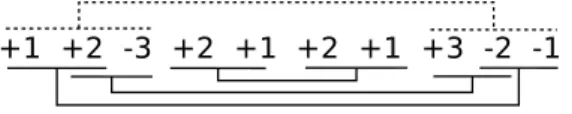
Fig. 3. All possibilities of assignment: XA= 1 (gene A occurs twice and signed genes are matched in the reading order), XB= 1 or XB = 0 (gene B occurs once) and XC = 0 (gene C occurs twice and signed genes are not matched in the reading order). Note that this construction is independent of the sign of the genes.
Proof. Let G1and G2 be two balanced genomes such that occ(G1) = 2 and let (χ, Φ) be the instance of Max-2-CSP obtained by MakeCSP(G1, G2). Let k be an integer.
Suppose there exists an assignment of χ such that at least k formulas ϕi ∈ Φ are satisfied. We create the following maximum matching (GM
1 , GM2 , M) of (G1, G2). For each variable Xg such that the gene g is duplicated, we match the occurrences of g in the reading order if Xg = 1 (such as gene A in Figure 3). If we have Xg = 0, we match the first occurrence of g on G1 with the second one on G2 and the second occurrence of g on G1 with the first one on G2 (such as gene C in Figure 3). Then, we match signed genes which are not duplicated. Now, we prove that each satisfied formula ϕi ∈ Φ induces a distinct adjacency for (GM
1 , GM2 , M). Let ϕi ∈ Φ be a satisfied formula which is defined in one of the cases (a), (b), (c) or (d) of the definition of MakeCSP:
– (a) We have ϕi = (Yij∧ Y j+1
i+1 ) and the duos di = (G1[i], G1[i + 1]) and dj = (G2[j], G2[j + 1]) are identical.
Here, we must prove that diand djare matched together in (GM
1 , GM2 , M) and thus induce an ad-jacency. First, we show that signed genes G1[i] and G2[j] are matched together in (GM1 , GM2 , M). Since ϕi is satisfied, we have Yij = 1. We must dissociate three cases: (i) the gene |G1[i]| is not duplicated: in that case, the signed gene G1[i] can be matched only with G2[j]. (ii) The gene |G1[i]| is duplicated and we have NG1[i] = NG2[j]. In that case, we have defined Yij = X|G1[i]| which implies X|G1[i]| = 1. Thus, since NG1[i] = NG2[j], the signed genes G1[i] and G2[j] are matched together. (iii) The gene |G1[i]| is duplicated and we have NG1[i] 6= NG2[j]. In that case, we have defined Yij = X|G1[i]| which implies X|G1[i]|= 0. Thus, since NG1[i] 6= NG2[j], the signed genes G1[i] and G2[j] are matched together. For each case, the signed genes G1[i] and G2[j] are matched together. We can conclude in the same way that G1[i + 1] and G2[j + 1] are also matched together, which implies that di induces an adjacency.
– (b) We have ϕi = (Yij+1∧Yi+1j ) = 1 and the duos di = (G1[i], G1[i+1]) and dj = (G2[j], G2[j+1]) are reversed.
We can use the same reasoning used in case (a) to prove that di induces an adjacency.
– (c) The duo di appears twice in G2 (noted dj and dj′). We have ϕi= (X|G1[i]|⊕ X|G1[i+1]|) and NG1[i] = NG1[i + 1].
Since ϕi is true, we have X|G1[i]| = X|G1[i+1]| which implies by construction of the maximum matching that di matches dj or dj′.
– (d) The duo di appears twice in G2 (noted dj and dj′). We have ϕi= (X|G1[i]|⊕ X|G1[i+1]|) and NG1[i] 6= NG1[i + 1]. Since ϕi is true, we have X|G1[i]|6= X|G1[i+1]|which implies by construction of the maximum matching that di matches dj or dj′.
Consequently, for each satisfied formula, there exists a distinct adjacency between GM
1 and GM2 . Thus, if there exists an assignment of χ which implies at least k satisfied formulas of Φ, then there exists a maximum matching of (G1, G2) which implies at least k adjacencies. ⊓⊔ Lemmas 11 and 12 prove that any α-approximation for Max-2-CSP implies an α-approximation for Max-2-Adj. In [9], an approximation algorithm is given for Max-2-CSP, whose approximation ratio is equal to 0.8741 ≤ 1.1442. Thus, we have the following theorem.
Theorem 7. Max-2-Adj is 1.1442-approximable.
5.2 A 3-approximation for Max-3-Adj
Now, we present a 3-approximation for Max-3-Adj by using the Maximum Independent Set problem defined as follows:
Problem: Max-Independent-Set Input: A graph G = (V, E).
Solution: An independent set of G (i.e. a subset V′ of V such that no two vertices in V′ are joined by an edge in E).
Measure: The cardinality of V′.
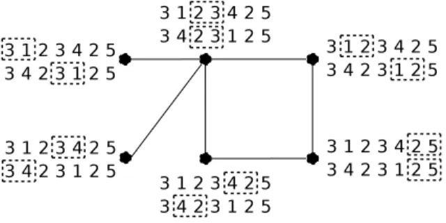
In [17], Goldstein et al. used Max-Independent-Set to approximate the Minimum Common String Partition problem by creating a conflict graph. We construct in the same way an instance of Max-Independent-Set where a vertex represents a possible adjacency and where an edge represents a conflict between two adjacencies. We define MakeMIS to be the following transformation which associates to two balanced genomes G1 and G2 an instance of Max-Independent-Set. We construct a vertex for each duo match, and then we create an edge between two vertices when they are in conflict, i.e. when two matches are incompatible. Figure 4 illustrates the graph obtained by MakeMIS(G1, G2) where G1 = +3 + 1 + 2 + 3 + 4 + 2 + 5 and G2= +3 + 4 + 2 + 3 + 1 + 2 + 5.
Fig. 4. The conflict graph obtained by MakeMIS(G1, G2) where G1 = +3 + 1 + 2 + 3 + 4 + 2 + 5 and G2= +3 + 4 + 2 + 3 + 1 + 2 + 5 (for sake of readability, positive signs are not displayed).
In order to prove that there exists a 3-approximation for Max-3-Adj, we give the following intermediate lemmas.