QUASARS WITH GAIA: IDENTIFICATION AND ASTROPHYSICAL PARAMETERS
J.-F. Claeskens1, A. Smette∗2, J. Surdej∗∗1
1Institut d’Astrophysique et de G´eophysique de Li`ege, Li`ege, Belgium 2European Southern Observatory, Santiago, Chile
ABSTRACT
Gaia will provide astrometric and photometric observa-tions for about 500 000 quasars distributed over the whole sky. The latter would constitute an isotropic grid of fixed sources perfectly suited to determine the referen-tial frame. However, they must first be properly identi-fied among stars, whose population is about 2000 times larger. Using broad and medium band photometry, we first compare the efficiency of two analysis methods (χ2
fitting and Artificial Neural Networks, ANNs) to produce the QSO catalogue with the lowest amount of contam-ination by stars. We then investigate whether the Gaia photometry could also provide precise values of the QSO astrophysical parameters (APs, like the redshift, the con-tinuum slope, the emission line strength and possibly the extinction). To reach that purpose, we also compare the performances of the Spectral Principal Component Anal-ysis (SPCA) with those of the χ2fitting and ANN
analy-sis.
Key words: Quasars; Astrophysical Parameters; Photom-etry.
1. INTRODUCTION
The end-of-mission Gaia data base will contain informa-tion on variability, astrometric posiinforma-tion, parallax, proper motion and photometry (in 5 broad bands [BBP] + 12 medium bands [MBP]) for about 500 000 quasars down to the magnitude G = 20. The bulk of the observed quasars is expected to be in the redshift range 1.5 – 2. This data set must be compared to the highly hetero-geneous set of 48 921 quasars gathered in the present version of the V´eron QSO compilation (V´eron-Cetty & V´eron 2003, including the set of 23 338 QSOs from the last 2dF release by Croom et al. 2004) and to the sam-ple of 100 000 QSOs to be observed at high latitudes in the north galactic hemisphere by the Sloan Digital Sky Survey (SDSS, York et al. 2000).
Although Gaia will only increase the total number of ∗Research Associate, F.N.R.S. (Belgium)
∗∗Research Director, F.N.R.S. (Belgium)
known quasars by less than one order of magnitude, and despite the fact that Gaia will not break the record of the highest QSO redshift, it has unrivalled advantages: (i) it will scan the whole sky and provide the most
ho-mogeneous QSO survey (including low galactic latitudes
where no optical survey has ever been carried out); (ii) the combination of the three independent, complemen-tary measurements that Gaia will produce (astrometry, variability, photometry) will likely allow us to build the most complete optically-selected survey down to G! 20. (iii) the end-of-mission angular resolution is excellent (S¨oderhjelm 2002); (iv) an astrophysical diagnosis (e.g., photometric redshift) is possible to some extent, without requiring spectroscopic follow-up.
Advantage (i) is not only crucial to obtain a dense, isotropic grid of fixed sources well designed to deter-mine the Gaia optical celestial reference frame, but also to study the matter distribution traced by the luminous QSOs on cosmological scales and, through later spec-troscopy, to detect intergalactic absorbing clouds located along their lines-of-sight.
Advantage (ii) will help to identify the most peculiar types of QSOs and study their populations. Indeed, reaching a high degree of completeness in a traditional QSO survey is usually difficult because of the large dif-ferences between the quasar spectra (due to redshift, vari-able galactic reddening, varivari-able absorption by interven-ing clouds along the line-of-sight, or due to intrinsic properties such as weaker emission lines [BL-Lac ob-jects], broad absorption lines [BAL] QSOs, red contin-uum QSOs and type II objects with narrow emission lines).
Advantage (ii) will also lead to a lower contamination rate of the QSO sample by specific stellar populations (e.g., white dwarfs at low redshifts, M stars at high red-shifts and early F stars for 2! z ! 3, where the Lyαline
is in the B filter) as compared with traditional broad band surveys. Given the fact that the QSO population does only represent 0.05% of the stellar population, building a
secure sample with 100% QSOs and without the help of a
spectroscopic follow-up requires a very efficient rejection algorithm. For comparison, the sample of colour-selected QSO candidates in the SDSS only contains 66% of true QSOs (Schneider et al. 2003).
Finally, we would like to stress that, thanks to advantages (i), (ii), (iii), it will be possible to identify with Gaia more than 900 gravitationally lensed quasars with an angular separation ∆θ ≤ 1"" between the images (provided that
an image of that size is telemetered to the ground). This number is an order of magnitude larger than the presently known number of lensed QSOs. Given the importance of strong gravitational lensing to probe the dark matter distribution in distant galaxies and given its sensitivity to cosmological parameters (see e.g., Claeskens & Surdej 2002 for a review), Gaia will significantly contribute to the field by providing the largest and most uniform opti-cal survey of lensed QSOs.
In the present study, we only deal with the
photomet-ric signature of QSOs present in the end-of-mission Gaia
data base. We use it (i) to select QSOs among stars as effi-ciently as possible (see Section 4) and (ii) to derive their astrophysical parameters (see Section 5). In Section 2, we present the libraries of synthetic spectra we have built (and which are available via the Gaia Photometric Work-ing Group (PWG) web site1). In Section 3, we briefly
de-scribe the analysis methods (χ2, ANNs, SPCA) and we
summarize our conclusions in Section 6.
2. SPECTRAL LIBRARIES
The diversity of the QSO spectra must be taken into ac-count to realistically test the Gaia performances. How-ever, there are no observed QSO spectral libraries cover-ing such a diversity over the full wavelength range sam-pled by Gaia (λλ 2400 – 10 500 ˚A). On the other hand, a check of the robustness of the classification algorithms is only possible if two totally independent sets of objects are available. Thus, we generated synthetic libraries based on two different approaches: the Modified Templates and the use of Spectral Principal Components.
2.1. Modified Templates (MT)
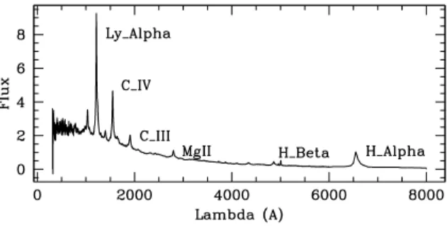
We first built a composite spectrum in the rest frame range 310 – 8000 ˚A, using four averaged observed spec-tra available in the literature (see Figure 1). We then subtracted the continuum by fitting the relation (Ferland 1996): C(λ)∝ !" λ λ0 #−α exp (−λX/λ) exp (−λ/λIR) + a $ (1) where α = 0.03 is the slope of the continuum, and we were left with an emission line spectrum E(λ), whose
total equivalent width W ! 10 000 ˚A. New spectra may then be generated by changing α and W in the observed ranges−4 < α < 3 and 2 < log W < 6 respectively2.
1http://gaia.am.ub.es/PWG/index.html
2The observed ranges of α and W have been derived from the
fit-ting of C(λ) and E(λ) to 3411 QSO spectra extracted from the SDSS DR1β. Most of the QSOs are found in the range−1 < α < 1 and 3000 < W < 10 000.
Figure 1. Composite QSO spectrum built from Cristiani & Vio (1990), Francis et al. (1991) and Zheng et al. (1997).
The resulting spectra is finally redshifted (0 < z < 5.5) and intergalactic absorption is added using the method described in Royer et al. 2000.
We then built two spectral libraries with 20 000 (resp. 17 325) spectra, corresponding to uniformly and ran-domly (resp. regularly) distributed values of the param-eters z, α and W . Those libraries are available on the PWG web site.
2.2. Spectral Principal Components (SPCs)
The (spectral) principal component analysis is a tech-nique useful to identify spectral features that correlate with each other. Different studies indicate that any given rest frame QSO spectrum can indeed be reasonably well described by a linear combination of a mean spectrum M (λ) and a set of principal components Pi(λ) (Francis
et al. 1992; Shang et al. 2003):
S(λ)∝ M(λ) + ' i=1,10 wiPi(λ) (2)
We made use of this property to create an independent library of 20 000 synthetic QSO spectra. Here we only used wiobtained by adjusting the Shang et al. SPCs to
the SDSS DR1β QSO spectra. However, the library con-tains spectra uniformly covering the range 0 < z < 5.5 instead of having the redshift distribution of the QSOs present in the SDSS DR1β. This library is also available on the PWG web site.
2.3. Stellar Libraries
Stellar contaminants must also be modelled. We con-sidered single ‘normal’ stars, binaries and white dwarfs (WDs). Again, we used synthetic spectra, respectively from the Basel Stellar evolution Library BaSeL2.2 (West-era et al. 2002) with 2000 K < T < 50 000 K,−1.02 < log g < 5.5, −5 < [M/H] < 1, from Malkov (see Jordi
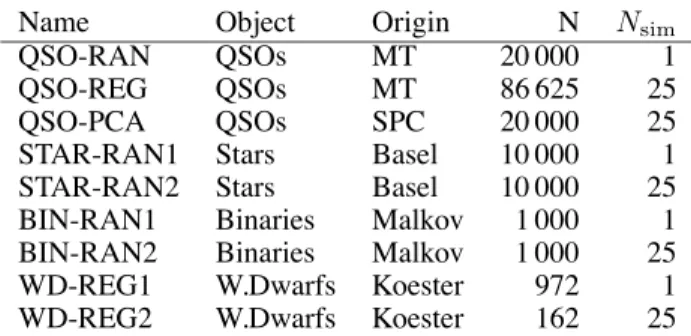
Table 1. Summary of the photometric data bases.
Name Object Origin N Nsim
QSO-RAN QSOs MT 20 000 1
QSO-REG QSOs MT 86 625 25
QSO-PCA QSOs SPC 20 000 25
STAR-RAN1 Stars Basel 10 000 1
STAR-RAN2 Stars Basel 10 000 25
BIN-RAN1 Binaries Malkov 1 000 1
BIN-RAN2 Binaries Malkov 1 000 25
WD-REG1 W.Dwarfs Koester 972 1
WD-REG2 W.Dwarfs Koester 162 25
et al. 2003a) and from pure-hydrogen atmosphere mod-els for degenerate stars (Koester, private communication), with 7000 K < T < 80 000 K and 7.5 < log g < 8.5.
2.4. Photometric Data Bases
From the synthetic spectra, the expected numbers of photo-electrons collected at the end of the Gaia mission are computed with the Gaia II revised simulator (June 2003; C. Jordi) in the 2B BBP system (Lindegren 2003), the 1X and the 2F MBP systems (Vanseviˇcius & Bridˇzius 2003; Jordi et al. 2003b)3. Dust extinction is added
at this stage with a uniform distribution in the range 0 < Av< 9 for normal and binary stars, and in the range
0 < Av< 2.5 for QSOs and WDs.
For all sets of spectra listed in Table 1, data bases have been generated without noise as well as for G = 18, 19 and 20 with realistic errors computed from the counts al-ready affected by noise. Limiting magnitudes have also been introduced. For test sets (TS), Nsim = 25, i.e., 25
realisations of the noise have been made for each entry in order to determine classification probabilities and uncer-tainties on the astrophysical parameters.
3. ANALYSIS METHODS 3.1. Nearest Neighbour (χ2)
The simplest approach for classification and parameter determination consists of comparing the observed flux vector fiwith the flux vectors Fijof each object j present
in the data base and selecting the one for which χ2= n ' filteri=1 " fi− Fij σi #2 (3)
is minimum. σi is the photometric error in filter fi.
This is the most popular minimum distance estimator, 3The choice of the BBP and MBP was not yet finalized at the time of
the simulations. The present design (4B and 2X or 3F) is not drastically different. However, there is one more filter and the wings of the 3F filters are steeper; this can only improve the efficiency of the algorithms proposed in this study.
also called ‘template fitting’. This is a local fitting in the sense that the result only depends on the local in-formation in the colour space. This method is powerful since it provides physical information on the associated template, it identifies degeneracies between templates, it works with missing data and it provides hints on unknown objects from their large distance to any known object lo-cus. However, the finite density of templates in the colour space is the dominating source of errors on the APs for bright objects (requires interpolation) and is the dominat-ing source of misclassification for faint objects. Given the number of operations, this method is slow.
3.2. Artificial Neural Networks (ANNs)
A supervised ANN can be considered schematically as a black box able to learn during a ‘training’ phase a non-linear relation between known inputs (here the flux vec-tors) and known outputs (here the type of the objects or the value of the APs), contained in a learning set (LS). Once the relation is learnt, new outputs can be quickly and reliably derived from new inputs, provided the latter are statistically compatible with the inputs of the LS (see e.g., Bishop 1995 for more details on ANNs). ANNs are complementary to the χ2-like approach in the sense that
they belong to the class of global fitting methods; ANNs are basically interpolaters whose characteristics are de-fined by the global, or statistical properties of the LS. This may seem more robust, but ANNs suffer from the so-called regularization problem. In practice, the train-ing must be tuned to learn the details of the distribution in the large dimensional colour space while not ‘memoriz-ing’ the exact distribution of the LS (overfitting). In such a case, the ANN would not recognize a slightly different object belonging to the same family. To reach that goal, we found three empirical rules: (i) complex problems should be broken into several simpler ones (e.g., succes-sive binary tests to reject well defined populations of stars and WDs instead of one ‘big classifier’); (ii) the data in the LS should be slightly noisier than in the test set (and therefore than in the sample that Gaia will observe); (iii) objects in the LS located on the edges of the parameter space are duplicated. However two weaknesses remain: ANNs are sensitive to missing input data, such as the lack of flux information in a filter, and they are unable to flag
unknown objects.
3.3. Spectral Principal Component Analysis (SPCA) Equation 2 shows how the QSO spectral information is contained in only a small number of wi. In turn, for a
QSO for which Gaia produces a set of fluxes in Nfilter
fil-ters, we can find the values of wiby resolving the
overde-termined linear system:
Akiwi= fk (4)
where fk is the observed flux in filter k and A is a
[Nfilter×(NPC+1)] matrix with element ki given by the
Table 2. Percentage of the different objects present in the TS to be found in the QSO class (1X+2B / 2F+2B).
Method G True STAR(%) True QSO(%) True WD(%) χ2 18 00.00 / 00.01 92.4 / 91.6 00.00 / 00.00 19 00.01 / 00.01 83.9 / 84.8 00.00 / 00.00 20 00.39 / 00.22 68.4 / 71.1 00.00 / 00.00 ANNs 18 00.00 / 00.03 68.5 / 83.0 00.00 / 01.23 19 00.00 / 00.03 62.5 / 59.2 00.00 / 00.00 20 00.00 / 00.02 31.8 / 40.4 00.00 / 00.00
the filter k. This computation is done after the averaged spectra M (λ) and each Pi(λ) have been redshifted and
multiplied by a function representing the absorption by the intergalactic medium. In practice, the inversion of Equation 4 must be done under the constraint of positiv-ity of the resultant spectrum.
This method is aimed at recovering the maximum of spectral information contained in the MBP. It may also be used to determine the redshift of the QSO. Indeed, when the assumed value of z is wrong, the system of equations (4) often can not be solved or yields unrealistic values of wi or χ2. The final adopted value for z is the one for
which a solution can be found for the wiand which
min-imizes χ2(z) = n ' filterk=1 ( ˆfk(z) − fk)2/σ2k (5)
where ˆfkis the reconstructed flux in filter k.
As shown in Section 5, this methods works quite well when a good signal to noise ratio is achieved in many filters, i.e., for z! 2.
4. QUASAR IDENTIFICATION
Whatever the method, the photometric identification of quasars among stars rely on the signature either of their strong emission lines (UV-excess like, for moderate red-shifts) or of the Lyα break absorption (large value of a
specific colour index: (B–V) for 3! z ! 4, (V–R) for 4! z ! 4.5, (R–I) for 4.5 ! z ! 6).
In the following, the LS consists of the data bases STAR-RAN1 + BIN-STAR-RAN1 + WD-REG1 + subset of 4000 QSOs from QSO-RAN, while the test set (TS) is built with the data bases STAR-RAN2+BIN-RAN2+WD-REG2+QSO-REG (see Table 1). The final class attribu-tion follows the rule:
QSO if PQSO > PST AR+ c and PQSO> PW D;
STAR if PST AR> PQSO− c and PST AR> PW D;
WD if PW D> PQSO− c and PW D> PST AR,
where PX is the relative frequency of attribution of the
class X among 25 simulations and 0 < c < 1 is a
con-trast parameter intended to minimize the stellar
contam-ination.
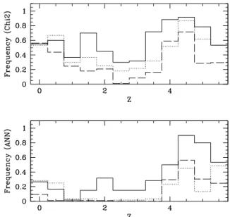
Figure 2. Redshift distributions of the QSOs found with the χ2method (top) and with ANNs (bottom) for G=20,
−0.5≤ α ≤ 0.5. Solid: 2500 ≤ W ≤ 10 000, AV = 0; dotted: 2500 ≤ W ≤ 10 000, AV = 2; dashed:
W < 2500, Av= 0.
In Table 2, the results are compared for different G mag-nitudes, for both the χ2 and the ANN methods and for
both photometric systems. The general trends are the fol-lowing: (i) the χ2method leads to a higher completeness
level (in the range∼70–90% depending on the magni-tude) but the ANNs are much better at rejecting contam-inating stars, virtually reaching a 0% contamination rate even at G = 20; (ii) white dwarfs are efficiently rejected with both methods; (iii) both photometric systems give similar results, although the 1X+2B is slightly better in terms of stellar rejection with the ANNs.
Figure 2 shows the redshift distributions of the QSOs found with each method at G = 20. The tribute to pay for a high stellar rejection rate is the loss of QSOs look-ing too much like a star, which is especially the case for 2 ! z ! 3 at ‘faint’ magnitudes. The QSO depletion is particularly severe with ANNs, as expected from their higher stellar rejection rate. Figure 2 also shows that with both methods the completeness is even smaller for red-dened QSOs (Av = 2) as well as for weak emission line
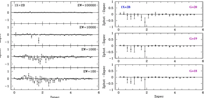
G=18 G=19
1X+2B G=20
Figure 3. Left: error on the photometric redshift obtained with the χ2method, as a function of spectroscopic redshift for typical QSOs in the QSO–REG data base (G = 19, α = 0 and Av = 0 and different values of W ; averaged values and 1σ error bars from the dispersion of 25 simulations). Right: same for the QSO-PCA data base (G = 18, 19 and 20; median values and quartiles from the dispersion within redshift-bins of ∆zbin= 0.25).
be more easily recognized, thanks to the strong and pe-culiar signature of the Lyαbreak; unfortunately, they will
not be very numerous because of the relatively bright lim-iting magnitude of Gaia.
With the χ2 method, the few contaminants at G = 18
are hot stars confused with BL-Lac QSOs while most of the contaminants at G = 20 are low metallicity reddened
stars ([F e/H] < −1 ;Av > 2) confused with reddened
QSOs whose intrinsic continuum is flat or red (α <− 1). When relaxing the contrast parameter with ANNs, the first contaminants are cold, low metallicity stars. The observed completeness of the QSO catalogue and the
observed stellar contamination rate depend on the
intrin-sic QSO and stellar AP distributions. The contamination rate also depends on the stellar to QSO population ratio, which is a function of the galactic latitude b. To get an idea of the expected results, we adopted the QSO APs distribution observed in the SDSS DR1β, we made use of the Besanc¸on Galactic Model (Robin et al. 2003) to predict the distribution of the stellar APs and we esti-mated the population ratio from the observed QSO num-ber count relation (Hartwick & Schade 1990) and the predicted stellar number count as a function of b from the Bahcall & Soneira (1980) model. With the χ2(resp.
ANN) method, the observed QSO completeness is found to range between 90% and 55% (resp. between 47% and 16%) for 18 < G < 20. The lower ANN completeness is due to the non-uniform observed redshift distribution4.
On the other hand, the stellar contamination should be maintained below 10−3% with the ANNs for any values
of G and b, while it ranges from a few per cent at large b 4A better completeness should certainly be achieved with ANNs by
including information on the redshift distribution in the LS, but we did not want to bias the searching algorithm at this level.
to 95% towards the bulge with the χ2method at G = 20.
Finally, an independent check using the QSO–PCA data base as TS leads to a completeness level in the range 92 – 70% (resp. 62 – 10%) with the χ2 (resp. ANNs) and 18 < G < 20. The drop in completeness at G = 20 (for a uniform z-distribution) with ANNs indicates the danger of working only with synthetic libraries.
5. ASTROPHYSICAL PARAMETERS
In this Section, the LS only consists of the QSO–RAN data base, while QSO–REG is the default TS and QSO-PCA is the independent TS. We shall not present results based on the ANN technique, since they are close to, but generally less good than, those obtained with the χ2
anal-ysis (see Claeskens et al. 2005 for more details). On the other hand, since the results are very similar between both photometric systems, we only show those relative to the 1X+2B system.
Among all QSO APs, the redshift is the most important one since it governs the QSO distance and luminosity through the cosmological model. It has the largest ef-fect on the QSO spectrum, so this parameter should also be the easiest one to determine on the basis of the Gaia photometry.
Figure 3 displays the expected errors on the photomet-ric redshift zphot as a function of the spectroscopic
red-shift zspec. The left graph shows that, unsurpinsingly,
zphotis best determined when zspec " 3 (i.e., when the
Lyα break enters the bluest filter) and for QSOs with
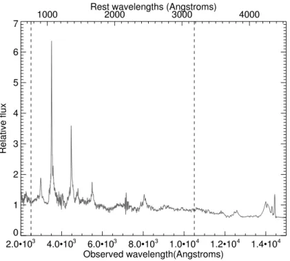
Figure 4. Example of a spectral reconstruction using the SPCA method. The shaded region represents the input spectrum (G = 19, zspec = 1.89, α = 0.03, W = 10 000) while the reconstructed spectrum is displayed with the solid line. The vertical dashed lines delineate the Gaia wavelength range.
0.5 ! zspec ! 2.5 reflects degeneracies coming from
the interplay between the limited wavelength coverage and coincidental wavelength shifts between strong emis-sion lines (e.g., λCIV/λLyα ! λC[III/λCIV! 1.25±0.2).
Those trends are amplified in the right graph, indepen-dently of the magnitude, which is a sign of systematic errors arising from the differences between the LS and the independent TS (QSO–PCA). Those differences can-not be avoided with synthetic libraries. A robust estimate of the error on zphot can only be derived in that
con-text. We find |∆z|Median ! 0.2 for 0.5 ≤ zspec ≤ 2
and|∆z|Median! 0.03 – 0.05 for zspec> 2.5.
The other QSO APs, namely the slope α, the total emis-sion line equivalent width W and the extinction AV have
only second order effects on the photometry. We thus expect their determination to be less accurate. We can only make predictions within the QSO-REG TS. For G = 19, −1≤ α ≤ 1, zspec < 2.5 and AV = 0, we
find|∆α|Median= 0.4 (W ≤ 3000) – 1.1 (W > 11000),
|∆W/W |Median= 1.8 (W ≤ 3000) – 0.6 (W > 11000)
and|∆Av|Median= 0.4 (W ≤ 3000) – 0.2 (W > 11000).
Those results confirm that those APs will be poorly con-strained with the Gaia MBP and BBP.
Finally, Figure 4 shows how a QSO spectrum (G = 19) can be retrieved from Gaia photometry by using the SPCA method and solving Equations 4 and 5. Although the results might be too optimistic because the spectra be-long to the set used to define the PCs, the method looks promising when the the S/N is good. It should be noticed that if the PCs are representative of the whole QSO fam-ily, spectral features may be constrained even out of the wavelength range covered by the Gaia photometric
sys-tems. Preliminary results indicate that the absolute error on zphot averaged over the range 0 < zspec < 2.3 is of
the order of 0.12 for typical QSO spectra.
6. CONCLUSIONS
Given the importance of creating from the data to be col-lected by Gaia the largest and purest sample of QSOs with their photometric redshifts (see Section 1), we inves-tigated in this first-step study the possibility to identify and characterize them, on the basis of their photometry
only (1X+2B or 2F+2B systems). To those ends, we built
synthetic spectral libraries and compared the χ2template fitting and the ANN methods. We also introduced the Spectral Principal Component Analysis. The results do not strongly depend on the adopted photometric system. First, we found that building a secure QSO catalogue based on photometry alone is possible, although the in-completeness can be severe, especially in the galactic plane where the reddening is expected to be higher. To that aim, ANN are more efficient than the χ2approach,
but the latter has a better completeness and could be used at high galactic latitude when the population ratio is more favourable to QSOs. It is however clear from this study that the photometry alone is not sufficient to reach a high degree of completeness, in particular for QSOs with 2! z ! 3 located close to the galactic plane, and it should be complemented with the variability and as-trometric constraints to be provided by Gaia. However, adopting σπ= 160 µas at G = 20, a 3σ measurement of
kpc. Since all stars hotter than M stars can be detected beyond that limit, their lack of apparent parallax will not distinguish them from QSOs. A model of the Milky Way will thus be necessary to quantify the probability for a given star to have no apparent parallax. The constraint on the proper motion looks more promising since most of the stars following the galactic rotation have a proper motion which will be detectable by Gaia. The galactic model should thus also include the stellar motion in order to estimate the probability that a given star has no appar-ent proper motion, which depends on the direction of the line-of-sight. This will be the aim of a second-step study. Second, this study has shown that the photometric red-shift of quasars can be reasonably well retrieved from the BBP+MBP photometry. The median absolute error on zphotis the largest for 0.5≤ zspec≤ 2 (|∆z|Median! 0.2
using the QSO–PCA independent TS). Unfortunately, this is the redshift range where most of the QSOs are expected! The reason is to be found in the interplay be-tween the limited wavelength coverage and the existence of casual multiplication factors between the wavelengths of several QSO strong emission lines. This degeneracy should be alleviated by adding photometric data farther in the ultraviolet. Such data are being obtained over the whole sky down to mAB = 20.5 by the GALEX satellite
(Martin et al. 2003). They should thus be included into the analysis of the Gaia photometry. Finally, we noted that the other QSO APs (α, W, AV) are much less
con-strained by the Gaia photometry. However, recovering at the same time the redshift and the weights of the spec-tral principal components seems promising for high S/N objects.
ACKNOWLEDGMENTS
It is a pleasure to thank Professor L. Wehenkel, who gave us access to the GTDIDT software, and L. Vandenbul-cke who made the first investigations with ANNs and other automatic classification algorithms. We also thank P. Francis and Z. Shang for kindly providing us with their QSO SPCs.
REFERENCES
Bahcall, J. N. & Soneira, R. M. 1980, ApJS, 44, 73 Bishop, C.M., 1995, ”Neural Networks for Pattern
Recognition”, Oxford University Press Claeskens, J.-F., Surdej, J., 2002, A&AR, 10, 263 Claeskens, J.-F., Smette, A., Surdej, J., 2005, A&A, in
prep.
Cristiani, S., Vio, R., 1990, A&A 227, 385
Croom, S. M., Smith, R. J., Boyle, B. J. et al. 2004, MN-RAS, 349, 1397
Ferland, G.J. 1996, Hazy, a Brief Introduction to CLOUDY 90, Univ. of Kentucky Physics Department Internal Report
Francis, P.J., Hewett, P.C., Foltz, C.B. et al. 1991, ApJ 373, 465
Francis, P. J., Hewett, P. C., Foltz, C. B., & Chaffee, F. H. 1992, ApJ, 398, 476
Hartwick, F. D. A. & Schade, D. 1990, ARAA, 28, 437 Jordi, C., Carrasco, J.M., Figueras, F., Bailer-Jones,
C.A.L., 2003a, Gaia technical report UB-PWG-014 Jordi, c., Grenon, M., Figueras, F., et al., 2003b, Gaia
technical report UB-PWG-011
Lindegren, L., 2003, Gaia technical report GAIA-LL-045 Martin, C. & GALEX Science Team 2003, American
As-tronomical Society Meeting, 203, #96.01
Robin, A. C., Reyl´e, C., Derri`ere, S., & Picaud, S. 2003, A&A, 409, 523
Royer, P., Manfroid, J., Gosset, E., Vreux, J.-M. 2000, A&AS 145, 351
Schneider D.P., Fan., X., Hall, P.B. et al.,2003, AJ 126, 2573
S¨oderhjelm, S., 2002, Gaia technical report DMS-SS-001 Shang, Z., Wills, B. J., Robinson, E. L. et al., 2003, ApJ,
586, 52
V´eron-Cetty, M.-P., V´eron, P., 2003, A&A 412, 399 Westera, P., Lejeune, T., Buser, R. et al., 2002 A&A 381,
524, 2002
York, D.G., Adelman, J., Anderson, J.E. et al., 2000, AJ 120, 1579
Zheng, W., Kriss, G.A., Telfer R.C. et al. 1997, ApJ 475, 469
Vanseviˇcius, V., Bridˇzius, A., 2003, Gaia technical report GAIA-VIL-008