Coupling an Unstructured NoSQL Database with a Geographic Information System
Amandine Holemans, Jean-Paul Kasprzyk, Jean-Paul Donnay
Geomatics Unit University of Liege
Liege, Belgium
email: [email protected], [email protected], [email protected] Abstract—The management of unstructured NoSQL (Not only
Structured Query Language) databases has undergone a great development in the last years mainly thanks to Big Data. Nevertheless, the specificity of spatial information is not purposely taken into account. To overcome this difficulty, we propose to couple a NoSQL database with a spatial Relational Data Base Management System (RDBMS). Exchanges of information between these two systems are illustrated with relevant examples involving spatial queries. The spatial data stored in MongoDB consists of field surveys (points, photos, etc.) and scanned plans, while reference data (cadastre) is recorded in PostGIS. The extensions required to allow this coupling are written in Python.
Keyword- Document-Oriented Database; MongoDB; Spatial RDBMS; PostGIS; Spatial Queries, Python.
I. INTRODUCTION
Like any Information System (IS), a Geographic Information System (GIS) uses a relational-type (RDBMS) or object-relational (O-RDBMS) database management system to store and manage spatial entities and their attributes. The database is based on a conceptual data model, written in UML (Unified Modelling Language) for example, where spatial entities are modelled by particular classes. In the physical database model, these classes are converted into spatial tables. According to the standards, the spatial footprint of entities is recorded in a dedicated field (GEOMETRY) in any spatialized table. This structure, relatively rigid, is suitable for any collection of entities always having the same fixed properties.
However, it appears in many projects that this inflexible structure does not lend itself to a large amount of heterogeneous information while remaining likely to be geo-located (Google, Facebook, etc.). This unstructured information, which can be described as documentation, can take the form of printed plans and diagrams, written reports, photographs, and so on. Whatever the origin, the documentation can always be scanned but in the form of a variable number of files in various formats.
Non-structured database management, known as NoSQL, has undergone a great development in recent years, particularly with the raise of voluminous and heterogeneous digital data (Big Data) [1]. Several recent systems have been designed for the management of documentation in its most various forms, even if the specificity of spatial information is not clearly addressed.
It is therefore possible to implement a GIS, based on an RDBMS, in parallel to a NoSQL system for the relevant documentation. The concern for many users is to choose between these two management systems to store and manage all the information [2]. However, it would be beneficial to couple these two systems in order to coherently associate and exploit the common spatial characteristics of these two types of information.
Our research objective consists precisely in proposing a coupling protocol between these systems as part of a pipe network management application.
In Section II, we describe the context of application that led us to propose this solution. Then, Section III takes stock of the specificities of NoSQL - particularly MongoDB software - compared to the standard RDBMS. Several scenarios are then presented in Section IV to illustrate the possibilities of exchanging information between a NoSQL system and a RDBMS, both in vector and in raster modes, while limiting data redundancy. Finally, we conclude in Section V with a discussion of the current capabilities and limitations of this type of coupling.
II. ABOUT THE APPLICATION
The issue of combining the management of a vector GIS and a documentation relating to this geographical information was posed to the AIDE company (Association
Intercommunale pour le Démergement et l’Epuration:
protection against floods caused by mining subsidence and management of the network of water sanitation, Liege Province, Belgium).
The company’s geographical objects (pipes, manholes, zones of intervention, etc.) are defined by vector geometries collected on the field by surveying techniques. In parallel, the GIS manages various reference data, such as cadastral objects and other administrative boundaries imported from institutional data providers.
The documentation includes survey blueprints and plans at different scales, geo-located digital photos and written reports that may include geo-located or geo-localizable information. This data – analogue or digital - is classified by projects. The projects are defined in time and space but the volume and the nature of the data constituting the documentation of a project vary very significantly, making a rigid data model unsuitable. Moreover, the projects are likely to interact or to merge in a planned way (e.g., renovation projects) or not (e.g., failures and various incidents on the
network). Due to all these considerations, the documentation associated with the projects appears as an unstructured set of data that must be related to reference data which, conversely, is structured according to an invariable scheme.
As part of a reengineering of the AIDE’s GIS, it was considered desirable to integrate the documentation into the database. It was at this point that the company asked us to examine the feasibility to couple NoSQL with a standard GIS solution.
III. STATE OF THE ART A. RDBMS versus NoSQL
Among the open source DBMSs that can handle spatial data, PostgreSQL and its PostGIS geospatial extension have great advantages. They give efficient functions, both in vector and in raster models, as well as a community offering a significant support [3]. In accordance with the OpenGIS Standard for "Simple Features for SQL", vector geometries are stored in the GEOMETRY field of spatialized tables. Since version 2.0, PostGIS can use two ways to store and process raster data: "in-db" or "out-db". In the first case, the raster data is stored in the RASTER field of spatialized tables, according to a principle similar to vector data storage. In the second case, only the metadata is stored in the database, the actual raster data being retrieved from the file system.
It is on PostgreSQL and PostGIS that the GIS of our application rests (version PostGIS 2.3.2 - PostgreSQL 9.6.3 at the time of application). Like all RDBMSs, however, it is not designed to handle large amounts of data for transactional processing. Indeed, SQL vertical scalability is limited with hardware improvement of the server (contrary to NoSQL horizontal scalability) [4]. In addition, the unstructured data leads to a considerable drop in performance (e.g., introduction of null values) or outrights practical impossibility. It is worth noting that RDBMSs remain effective in decision-making on large data warehouses [5].
First, NoSQL has developed to cope with large amounts of data [6]. Then, the need for simpler and less rigid models has strengthened the development of unstructured database models [7]. The term NoSQL groups various unstructured database families that can be characterized by their schema type. There are currently 4 families: key-value, column, graph and document-oriented databases [8]:
Key-value-oriented: They constitute the simplest schema where a key refers to a particular type of value. This type of schema offers quite limited query capabilities.
Column-oriented: This is an extension of the key-value schema by allowing a key to return multiple values.
Graph-oriented: The diagram is here in the form of a graph composed of edges and nodes.
Document-oriented: These databases are composed of keys that refer to a document, which can itself contain multiple embedded documents. Collections thus gather several documents from the same family, but their internal structure may vary. They do not require schemas beforehand and have a structure able to evolve over time without excessive costs. In addition, the contents of the document can be scrutinized by queries.
B. MongoDB
In the AIDE application briefly described above (II) the problem comes from the management of a variable documentation in quantity and content, essentially attached to the point objects (manholes). The network aspect is not explicitly exploited so that the solution chosen for our analysis is based on a document-oriented and not a graph-oriented database as one might have imagined at first glance with a pipe network management company. The choice of the document-oriented DBMS focused on MongoDB (version 3.4; [9]). This DBMS is easy to handle thanks to the various drivers available and its installation facilities. It does not have its own query language, but adapts to the chosen driver. MongoDB also uses standard formats (JavaScript Object Notation – e.g., JSON), which can be interesting for the expected manipulations. Currently, this NoSQL DBMS is the most popular one in the NoSQL category. It offers a large community making its use easier [10].
Presently, the geospatial domain is not a priority in the design of a NoSQL DBMS. Systems sometimes have an extension to manage geographic data while in other systems these features are natively included [11]. MongoDB is able to natively manage geospatial data, but dedicated processing is quite limited as soon as non-point geometries are concerned [12]. These limits come from the lack of maturity of this type of DBMS, but it is obviously constantly evolving.
MongoDB can spatially index and process vector geometries in 2 coordinate systems, labelled 2D and 2DSphere. In 2D, the coordinates (x, y) are local (not attached to a spatial reference system) and are described as legacy coordinate pairs in JSON. In 2DSphere, the coordinates are expressed in the geodetic system WGS84 (EPSG: 4326) and are described in GeoJSON. Elementary spatial predicates (within, near) are applicable to both domains, but the intersection is only possible in 2DSphere.
Raster geospatial data is not explicitly recognized by MongoDB. However, images can be manipulated in many ways by this software [13]. The image file can either (1) be managed by the file system, out of the database, or (2) be embedded in binary form in a MongoDB document if it is not too large (16 Mb maximum, and it is even recommended not to exceed 1 Mb), or (3) be incorporated into a document managed by the GridFS method.
With GridFS, the files, written in BSON (Binary JSON) format, can be much bigger, and a larger number of files can be managed in one directory [13]. The files are actually divided into several chunks, gathered in one “fs.chunk” collection, while the document metadata, notably allowing grouping the chunks, are the subject of a separate “fs.files” collection [14]. GridFS processes files and their metadata at the same time [15]. The facilities offered by GridFS are implemented in all official MongoDB drivers and a GridFS management tool, called Mongofile, is also available [16]. It should be noted in passing that the document management method via GridFS is particularly well suited to the classification of project-based documentation as carried out by the company AIDE.
It should be noted further that any image in MongoDB can be geo-located by a point in WGS84 coordinates (e.g., a geo-located photograph). But except for this location point, the image geospatial data are not necessarily geo-referenced in the WGS84 datum.
C. Drivers and Interfaces
Several extensions exist to interface MongoDB but they are not yet fully satisfactory. For a quick check, Compass for example, can be handy. But for maximum interactivity, it is desirable to work directly with a server language. C++, Java, Python, Perl or PHP, for example, may be perfectly suitable. For visualizing geospatial data from MongoDB, an Open Source GIS application should be a good solution. For instance, QGIS has a long history of extensions to PostGIS and is currently offering four extensions dedicated to MongoDB. But they do not seem to be perfect yet [17].
In this application, we have retained Python language. It is enough to import the drivers PyMongo and Psycopg2 in the same routine to provide a common interface to the couple of databases. Note that it is also in Python that the QGIS extensions can be written.
IV. EXAMPLES OF SPATIAL INTERACTIONS
In order to illustrate the coupling of the two systems, MongoDB and PostGIS, we have selected some types of data contained in the application of the AIDE company. The spatial data likely to feed MongoDB is either scanned plans, georeferenced (Geo-TIFF format) or not, and field data: manholes in point form (vector format) and photographs (image/raster format) geo-located on a point. The spatial data stored in PostGIS are reference data, from which we have selected the cadastral data [18] in vector form. It should be mentioned that the cadastre does not cover the public domain and that, consequently, the vector entities surveyed by the AIDE (manholes and pipes) are not located on the cadastral territory.
A. Vector interactions
The interactions will be done in both directions: from MongoDB to PostGIS and vice versa.
1) From MongoDB to PostGIS:
A simple query example consists in identifying the cadastral parcels (preserved in PostGIS) that are located in
the vicinity of a point (e.g., manhole) whose coordinates are stored in MongoDB (Figure 1).
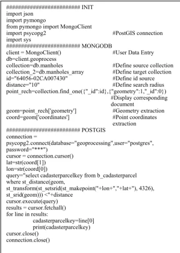
The Python routine first selects the point using a MongoDB request. Its WGS84 coordinates are received in GeoJSON format and are associated to a PostGIS point after conversion in the user’s reference system (recorded in the parcel metadata). Python interrogates the user on the search radius and launches the PostGIS request to select the parcels (to reduce the listing size (Table I), the interactive data entry is replaced by predefined constants).
TABLE I. PYTHON SCRIPT LOOKING FOR PARCELS IN POSTGIS WITHIN A CERTAIN DISTANCE OF A POINT RECORDED IN MONGODB. ######################### INIT
import json import pymongo
from pymongo import MongoClient
import psycopg2 #PostGIS connection import sys
######################### MONGODB
client = MongoClient() #User Data Entry db=client.geoprocess
collection=db.manholes #Define source collection collection_2=db.manholes_array #Define target collection id="64056-02CA007430" #Define id source distance="10" #Define search radius point_rech=collection.find_one({"_id":id},{"geometry":1,"_id":0})
#Display corresponding document
geom=point_rech['geometry'] #Geometry extraction coord=geom['coordinates'] #Point coordinates
extraction ######################### POSTGIS connection = psycopg2.connect(database="geoprocessing",user="postgres", password="***") cursor = connection.cursor() lat=str(coord[1]) lon=str(coord[0])
query="select cadasterparcelkey from b_cadasterparcel where st_distance(geom,
st_transform(st_setsrid(st_makepoint("+lon+","+lat+"), 4326), st_srid(geom))) <"+distance
cursor.execute(query) results = cursor.fetchall() for line in results:
cadasterparcelkey=line[0] print(cadasterparcelkey) cursor.close()
connection.close()
Figure 1. Selection of parcels in PostGIS in the vicinity of a selected point from MongoDB (search radius provided by the Python routine).
2) From PostGIS to MongoDB:
The reverse query should identify the point(s) (MongoDB) located near a cadastral parcel (PostGIS).
The notion of proximity is easily translated by the definition of a buffer around the cadastral parcel. However, this simple operation cannot be achieved in MongoDB. It is then entrusted to a POSTGIS request and the coordinates of the obtained polygon are converted into WGS84 in GeoJSON format to query MongoDB. In this example, the MongoDB request (within operator) will have to identify the geo-location points of the photographs taken within the buffer polygon (Figure 2).
Figure 2. Selections of photographs (point georeferenced in MongoDB) falling in a buffered parcel in PostGIS.
B. Raster interactions
The documentation of AIDE company is essentially composed of scanned plans and it is essentially around these that the interaction is sought. However, it must be remembered that scanned plans are available at multiple scales: small-scale assembly plans, large-scale detail plans. This multi-scale cover can be organized as embedded documents in MongoDB. In addition, the plans cover areas of interest that are not necessarily rectangular, so the scanned images likely incorporate portions without data (No-Data). Finally, the plans are not systematically georeferenced after scanning. As a result, the edges of the image are generally not parallel to the axes of the reference coordinate system.
1) Raster / Vector interactions:
A priori, for general queries concerning the presence of geographical objects within the plan, in one way or the other, it suffices to define the neatline (according to the OGC encoding best practices [19]) defining the border of the raster file and to confront it with the geometry of the vector objects preserved in PostGIS. The neatline is made of a series of point coordinates in clockwise order. The minimum of two points is considered as the diagonal of the minimum bounding rectangle (MBR), which assumes that the sides of the raster are parallel to the axes of the projected coordinate system. The coordinates of the neatline and the user's Spatial Reference Identifier (SRID), are provided to PostGIS to build a polygon in the GEOMETRY field of a spatial table (Figure 3). It is then possible to easily check the occurrence of vector objects within the polygon via a general purpose
2D clipping algorithm, such as the Weiler’s algorithm [20] in the PostGIS environment.
On the other hand, if the query involves the value of the pixels of the scanned plan (to avoid the No-Data values for example), it is necessary to make the georeferenced scanned plan accessible to PostGIS or to replicate it in a RASTER field of a raster table. These cases are discussed below and because the image neatline can be obtained by the raster function “st_enveloppe” in PostGIS, it will be no longer necessary to store the neatline in a vector spatial table.
2) Georeferenced scanned plan:
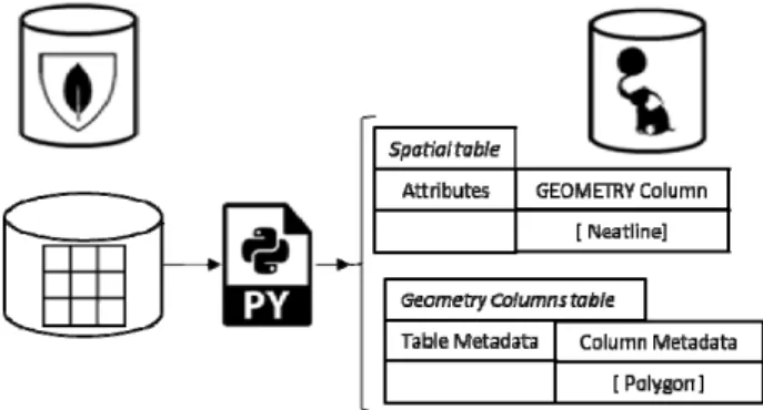
The scanned plan can be georeferenced and available e.g., in Geo-TIFF format. If it is managed by the MongoDB file system, it allows an immediate sharing solution with the PostGIS environment because of its ability to access, from the RASTER field, to external files (out-db alternative – Figure 4). If the image file is managed by GridFS in MongoDB, it is desirable to export it from the database in order to share it with PostGIS. This is achieved by a Python script listed below (Table II).
Figure 3. Preservation of the neatline (polygon) of a scanned plan (MongoDB) in the GEOMETRY column of a spatial table (PostGIS).
######################### INIT import pymongo
from pymongo import MongoClient from bson import objectid import gridfs
from os.path import basename import os
from bson.objectid import ObjectId from io import BytesIO
######################### EXPORT
conn = MongoClient() #Connection to MongoDB & GridFS db = conn.geoprocess
fs = gridfs.GridFS(db, "plan") #Connection to image file in DB gridout = fs.get(ObjectId("5a1ee153a9e79f1934cdf3a1"))
#Read file with objectId fout = open('plan_mongo.tiff', 'wb')
#Open TIFF file fout.write(gridout.read() #Write TIFF file fout.close()
TABLE II. PYTHON SCRIPT EXTERNALIZING AN IMAGE MANAGED BY GRIDFS AS A TIFF FILE.
3) Un-referenced scanned plans and World File:
If the scanned plan is not georeferenced, it is necessary to proceed to this geo-registration under PostGIS. This involves, on the one hand, communicating to PostGIS the necessary parameters and, on the other hand, transmitting the image file itself, exported from MongoDB.
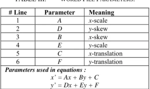
Regarding the registration parameters, the proposed solution is to enrich the metadata of the plan with the corresponding World File resuming the 6 parameters of the affine transformation between the image-coordinates and the user’s projected coordinates [21] (Table III).
TABLE III. WORLD FILE PARAMETERS.
# Line Parameter Meaning
1 A x-scale 2 D y-skew 3 B x-skew 4 E y-scale 5 C x-translation 6 F y-translation
Parameters used in equations : x’ = Ax + By + C y’ = Dx + Ey + F
At the choice of the user, the World File parameters can be computed from the neatline coordinates by the Python script (the neatline is generally easier for the user to specify than the 6 parameters of the transformation matrix). In addition, the destination SRID must be specified to PostGIS.
Figure 5. A Python routine uses World File parameters to create a georeferenced raster in PostGIS (TIFF/TFW format is an example).
As in the previous example, the image in MongoDB can be managed as an external file or more likely, to meet the
company's project-based management, managed by the GridFS method. In the latter case, it is still necessary to reconstitute the image in a file which is external to the database. The Python script transmits it to PostGIS which
Figure 4. MongoDB and PostGIS share an external GeoTIFF File.
######################### INIT import psycopg2
import os import subprocess import pymongo
from pymongo import MongoClient from bson import objectid import gridfs
from os.path import basename import os
from bson.objectid import ObjectId from io import BytesIO
######################### MONGODB
conn = MongoClient() #Connection to MongoDB & GridFS
db = conn.geoprocess fs = gridfs.GridFS(db, "plan")
gridout = fs.get(ObjectId("5a1ee153a9e79f1934cdf3a1")) filelist=fs.list() #List all files in the collection print (filelist)
fout = open('plan_mongo.tiff', 'wb') #Open TIFF file fout.write(gridout.read()) #Write TIFF file fout.close()
world= open("C:/Projets/geoprocessing/donnees/plans/world/02014-01-I003_01_ech1000-V1(1).wld",'r') #Open World File
read_data=world.read() #Read World File world_list=read_data.split("\n") #Create parameters list ######################### POSTGIS
xscale=world_list[0] #A # Read georegistration parameters yskew=world_list[1] #D xskew=world_list[2] #B yscale=world_list[3] #E xtranslate=world_list[4] #C ytranslate=world_list[5] #F srid="31370"
db_name = 'geoprocessing' # Connection to PostGIS db_host = 'localhost' db_user = 'postgres' db_password = '***' connection = psycopg2.connect(database=db_name,user=db_user, password=db_password) cursor = connection.cursor()
query="drop table if exists public.test" #Delete previous test table cursor.execute(query)
connection.commit()
#Import raster in test table os.environ['PGPASSWORD'] = db_password # Set pg password environment variable
cmd = 'raster2pgsql plan_mongo.tiff public.test | psql -U {} -d {} -h {} -p 5432'.format(db_user,db_name,db_host)
subprocess.call(cmd, shell=True)
# Georegistration of the test table query="update test set rast=st_SetGeoReference(rast,'"+xscale+" "+yskew+" "+xskew+" "+yscale+" "+xtranslate+" "+ytranslate+"', 'GDAL') where rid=1"
cursor.execute(query)
#Assign SRID to the test table query="update test set rast=st_setsrid(rast, "+srid+") where rid=1" cursor.execute(query)
cursor.close()
TABLEIV. PYTHON SCRIPT TAKING A TIFF FILE FROM MONGODB AND USING WORLD FILE PARAMETERS TO GEO-REFERENCE A RASTER IN
stores the temporary image in a raster table. Then the script invokes the PostGIS function "st_setgeoreference" with the World File parameters to update a georeferenced version of the image with its proper metadata (Figure 5). The process is detailed in the last listing (Table IV).
V. CONCLUSION
As soon as a language offers drivers for PostGIS and MongoDB, which is the case of Python used here, it is technically easy to couple the two databases with a single interface. However, the sharing of geospatial data is not immediate because MongoDB introduces some limitations.
In vector mode, the 2DSphere coordinate system implies the use of geodetic coordinates WGS84, which is impractical and confusing in calculations on non-point geometries. It is likely a corollary that the facilities offered for geometries other than points are so undeveloped. However, the combined functionalities offered by MongoDB and PostGIS are enough to obtain a fast and satisfactory result for simple queries on points. But if objects with complex geometries are included in the MongoDB database, it is clear that currently, their replication in PostGIS is the best or the only solution to allow serious spatial processing.
MongoDB does not explicitly recognize geographic raster data. The proposed solution is to manage a georeferenced file (e.g., GeoTIFF) by the MongoDB file management system. If it is managed by GridFS, it is first necessary to reconstitute an external image file through MongoDB commands. Then, the file can be shared without replication by PostGIS which will take care of all the required spatial processing. On the other hand, if the raster data is stored in a non-georeferenced image file in MongoDB it will be necessary to entrust this geo-registration to PostGIS using enriched metadata, which significantly increases the operations and creates unnecessary redundancy.
Geo-visualization is also problematic in MongoDB. Our proposal is to assimilate the Python interface common to both databases, to an extension of QGIS. However, the investment in the development of a general extension is jeopardized by the rapid evolution of the NoSQL systems in general, and MongoDB in particular. But the fast and multiple updates experienced by these systems are in themselves a good thing that should progressively remove the locks registered today on geospatial information.
ACKNOWLEDGEMENT
AIDE is thanked for allowing us to carry out this study and for providing the necessary data and documents. The digitized cadastral plans (version 01/01/2016) were provided for educational purposes by the General Administration of Heritage Documentation (AGDP) as a manager of the authentic source.
REFERENCES
[1] A. B. M. Moniruzzaman and S. A. Hossain, “NoSQL Database: New Era of Databases for Big data Analytics – Classification, Characteristics and Comparison”, International Journal of Database Theory and Application, Vol. 6, No. 4, 2013.
[2] S. Agarwal, and K. S. Rajan, "Performance analysis of MongoDB versus PostGIS/PostGreSQL databases for line intersection and point containment spatial queries,” Spatial Information Research, 24 pp. 671-677, 2016.
[3] Postgis-users – PostGIS Users Discussion. [Online]. http://lists.osgeo.org/mailman/listinfo/postgis-users [retrieved 01, 2018].
[4] C. Birgen, H. Preisig and J. Morud, “SQL vs. NoSQL”. Norwegian University of Science and Technology, Scholar article, 42 p., 2014. [5] R. Kimball, and M. Ross, “The Data Warehouse Toolkit: The
Definitive Guide to Dimensional Modeling,” New York: John Wiley & Sons, 3d ed., 2013.
[6] A. Oussous, F.-Z. Benjelloun, A. Ait Lahcen, and S. Belfkih, "Comparison and Classification of NoSQL Databases," International conference on Big Data, Cloud and Applications (Tetouan, Morocco), pp. 1-6, May 2015.
[7] S. Gupta, and G. Narsimha, "Efficient Query Analysis and Performance Evaluation of the Nosql Data Store for BigData," Proceedings of the First International Conference on Computational Intelligence and Informatics (Singapore), S. C. Satapathy et al. (eds.), pp. 549-558, 2017.
[8] P. Amirian, A. Basiri, and A. Winstanley, "Evaluation of Data Management Systems for Geospatial Big Data," Computational Science and Its Applications (ICCSA), Springer International Publishing, pp. 678-690, 2014
[9] MongoDB, “MongoDB Documentation”. [Online]. https://docs.mongodb.com/ [retrieved 01, 2018]
[10] L. Bonnet, A. Laurent, M. Sala, B. Laurent, and N. Sicard, "Reduce, You Say: What NoSQL Can Do for Data Aggregation and BI in Large Repositories", Proceedings of 22nd International Workshop on Database and Expert Systems Applications (DEXA), IEEE, pp. 483-488, 2011.
[11] C. de Souza Baptista, C. E. Santos Pires, D. Farias Batista Leite, M. Guimares de Oliveira, and O. F. de Lima Junior, "NoSQL Geographic Databases: An Overview," E. Pourabbas (ed.), Geographical Information: Trends and Technologies, CRC Press, pp. 73-103, 2014.
[12] MongoDB, “Migration Guide from RDBMS to MongoDB (Guide de migration d’un système RDBMS vers MongoDB).” 2015. [Online]. https://www.mongodb.com/collateral/rdbms-mongodb-migration-guide/[retrieved 01, 2018].
[13] K. Banker, P. Bakkum, S. Verch, and T. Hawkins, “MongoDB in action,” Manning Publications Co, 2016.
[14] W. Xin, “Design and Implementation of CNEOST,” Chinese Astronomy and Astrophysics, 38, pp. 211-221, 2014.
[15] G. Kloss, “MataNui – A Distributed Storage Infrastructure for Scientific Data,” Procedia Computer Science, 18, 2607-2610, 2013.
[16] C. Dasadia, and A. Nayak, “MongoDB Cookbook,” 2d edition, Packt Publishing, 2016.
[17] QGIS, QGIS Python Plugins Repository [Online]. https://plugins.qgis.org/ [retrieved 01, 2018].
[18] Service Public Fédéral Finance, “CadGIS”. [Online]. http://ccff02.minfin.fgov.be/cadgisweb/ [retrieved 01, 2018].
[19] Open Geospatial Consortium, “PDF Georegistration Encoding Best Practice Version 2.2, OGC 08139r3,” G. Demmy, and C. Reed, (eds), 2011.
[20] J. D. Fooley, A. van Dam, S. K. Feiner and J. F. Hughes, “Computer Graphics. Principles and practice,” Addison-Wesley, 2d ed., 1992.
[21] Library of Congress, “ESRI World File,” Sustainability of Digital Formats: Planning for Library of Congress Collections,” 2015. [Online]. https://www.loc.gov/ preservation/digitalformats/fdd/fdd000287.shtml [retrieved 01, 2018].