Risk assessment of groundwater pollution using sensitivity analysis and a worst-case scenario analysis

Texte intégral

(1)Risk assessment of groundwater pollution using sensitivity analysis and worst case scenario analysis MARIJKE HUYSMANS (1) , TAMÁS MADARÁSZ (2) AND ALAIN DASSARGUES (1,3) (1) Laboratory for Hydrogeology, Department of Geology-Geography, Faculty of Exact Science, Catholic University of Leuven, Redingenstraat 16, 3000 Leuven, Belgium (2) Department of Hydrogeology and Engineering Geology, University of Miskolc, Miskolc, Hungary (3) Hydrogeology and Environmental Geology, Department of Georesources, Geotechnologies and Building Materials (GEOMAC), University of Liège, B52/3, Liège, Belgium marijke.huysmans@geo.kuleuven.ac.be 0032 16 32 64 49 0032 16 32 64 01. This paper illustrates how sensitivity analysis and worst case scenario analysis can be useful tools in risk assessment of groundwater pollution. The approach is applied to a study area in Hungary with several known groundwater pollution sources and nearby drinking water production wells. The main concern is whether the contamination sources threaten the drinking water wells of the area. A groundwater flow and transport model is set up to answer this question. Due to limited data availability, the results of this model are associated with large uncertainty. Sensitivity analysis and worst case scenario analysis are applied to estimate this uncertainty and to build confidence in the model results.. 108 words in abstract. Keywords: sensitivity analysis, worst case scenario analysis, groundwater pollution, groundwater and transport modeling. 1.

(2) 1. Introduction Determining the environmental risk associated with groundwater pollution is a common research question. This usually involves investigating whether the polluted groundwater can reach drinking water wells, rivers, houses, ecologically vulnerable zones or fauna and flora (Calow 1998). Computer models are commonly used to make such predictions regarding groundwater flow and contaminant concentrations. Lack of input data and heterogeneity of the model parameters causes however uncertainties associated with the results of those models. The uncertainty associated with predictions is often overlooked, despite the fact that an assessment of such uncertainty may be critical (Levy et al. 1998), especially in situations with relatively scarce data. Several techniques are available to deal with model and parameter uncertainties. A common probabilistic approach for assessing uncertainty is Monte Carlo simulation (Asante-Duah 1998). This technique consists of randomly choosing input values from input probability distributions and calculating the output for each realization. Repeated runs provide a distribution of the outcome. Although Monte Carlo simulation is robust and asymptotically convergent, it lacks computational efficiency. Moreover, probability functions of each model parameter are required and this may be an important disadvantage in situations with scarce input data. Monte Carlo simulation is often combined with a geostatistical approach. Geostatistics require however extensive datasets to properly describe the spatial variability of each parameter and such databases are unfortunately not always available in real case studies. Fuzzy number based methods (e.g. Dou et al. 1995) and first- and second-order reliability methods (e.g. Ünlü et al. 1995) are efficient alternatives to Monte Carlo simulation, but these methods are usually not common knowledge of most practitioners. A fast and straightforward approach to deal with uncertainty is sensitivity analysis and/or worst case scenario analysis. Sensitivity analysis examines the relative change or response of output variables caused by variation of the input variables and parameters. It is a technique that tests the sensitivity of an output variable to the possible variation in the input variables of a given model. Performance of sensitivity analysis requires data on the range of values for each 2.

(3) relevant model parameter (Asante-Duah 1998). In worst case scenario analysis, each model variable and parameter is given the worst possible value, which results in the most unfavorable model outcome with respect to the particular purpose of the model. Performance of this technique only requires an idea of the worst possible case values. In this paper, a risk assessment approach based on sensitivity analysis and worst case scenario analysis is applied. The study area is the city of Mateszalka, a city of 25,400 inhabitants. It is situated in eastern Hungary, near the border of Romania and Ukraine. Mateszalka lies along the Kraszna River, a small river that discharges into the Tisza River, which flows into the Danube. Mateszalka encloses several known possible groundwater pollution sources. A first groundwater pollution source in the area is the municipal waste disposal site. This landfill has a volume of 800,000 m³. It has no appropriate lining system and the groundwater level reaches the bottom of the waste during wet periods (Nauner 2000). A second groundwater pollution source is the former sewage oxidation pond. From 1971 to 1997, the sewage of the city was disposed in this pond in order to be aerated (Nauner 2000). Now this pond is covered with soil and plants but large volumes of sewage sludge are probably still present in the subsoil. A third groundwater pollution source is the sewage treatment plant where sewage undergoes preliminary and primary treatment. Preliminary treatment is the removal of solids like wood, paper, rags and plastic by screens. Primary treatment consists of the separation of the remaining solids from the liquid by passing the sewage through large settlement tanks, where most of the solid material sinks to the bottom. About 70% of solids settle out at this stage and are referred to as sludge. 10,000 m3 of this sludge is stored at the site (Nauner 2000). Houses that are not connected to the sewage treatment system are a fourth groundwater pollution source. In 2000, more than 20% of the houses of the area were not connected to this system (Nauner 2000). The cesspits are not covered with concrete, so that the sewage can easily reach the groundwater, particularly because of the high groundwater level. Industrial activities are a fifth groundwater pollution source. The main question to be answered is whether these contamination sources threaten the nearby drinking water wells, which are screened at a depth of approximately 200 to 260 m in a. 3.

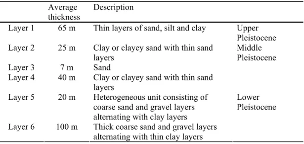
(4) very permeable aquifer consisting of coarse grained sand and gravel. This study was complicated by limited data availability.. 2. Geology Matesalka is situated in the Great Hungarian Plain, which is part of the Pannonian intermountain basin. The Pannonian basin is a topographically low region which is about 400 km from north to south and 600 km from west to east. In the region under study, the Pleistocene sediments have a thickness of approximately 260 m. The Lower Pleistocene has a thickness of approximately 110 m, the Middle Pleistocene has a thickness of 90 m and the Upper Pleistocene is about 60 m thick. The Lower Pleistocene is an aquifer system with coarse grained layers on a regional scale. The sediments are alluvial deposits consisting mainly of gravel and coarse sand. The Lower Pleistocene is the most permeable sequence of the area and is therefore the most important aquifer for local drinking water production. The Middle Pleistocene has a totally different nature than the Lower Pleistocene. It is made up of silt and silty clay aquitards of low permeability. These deposits are both alluvial and lacustrine sediments. The Upper Pleistocene is composed of medium to fine grained sand and silt. These alluvial sand deposits are aquifers, but with a lower permeability than the Lower Pleistocene. The underlying clayey Pliocene is considered as an aquitard and serves as an impermeable bottom boundary in the groundwater flow and transport models. The geometry of the different geological layers was assessed by borehole data from 23 wells (Fig. 1). The complex geology was simplified by dividing the Pleistocene into 6 hydrostratigraphical units (Table 1). Layer 1 is a heterogeneous aquifer which consists of many thin layers of sand, silt and clay. This layer is quite permeable, as is confirmed by the numerous well filters that are present in this layer. Layers 2 and 4 consist mainly of clay and sandy clay layers and are therefore the least permeable units. No wells are screened in these layers, which act as aquitards. Layer 3 is a continuous sand layer that occurs in every well log. This last layer is used for water extraction by a few wells. Layer 5 and 6 are the best aquifers or the units with the highest hydraulic conductivity. All the drinking water, extracted by the local water company, is extracted from these 2 layers. 4.

(5) Figure 1 Table 1 3. Groundwater flow model The differential equations describing groundwater flow are solved by MODFLOW (McDonald & Harbaugh 1988), a block-centered finite-difference method based software package.. 3.1 Boundary conditions The hydrogeological model is a local model of 9 km x 10 km x 260 m. The top of the Pliocene clay deposits represents the impermeable bottom of the model due to the low permeability of this unit. Prescribed piezometric head conditions are applied at the boundaries of the permeable layers 1, 3, 5 and 6. The piezometric heads at the boundaries are deduced from nearby piezometers and regional and local piezometric maps and profiles. The boundaries of layers 2 and 4 are zero flux boundaries. These layers consist primarily of clay and therefore groundwater flow is insignificant relative to the other layers and primarily in the vertical direction. Therefore the flux across the boundary of these clayey layers is assumed to be zero. The model is bordered in the east by a river. This river has a slope of 13 cm/km and a width of 10 to 20 m. The river bottom sediments have a thickness of approximately 0.7 m and a hydraulic conductivity of about 10-6 m/s. Specified river levels are assigned along the river based on interpolation of nearby river stage measurements. Groundwater abstractions in the well field are entered in the model based on monthly abstraction data. There are 15 abstraction wells with a total capacity of 15,000 m3/day. An estimation of the recharge of the aquifer of 30 mm/year is found by applying Thorntwaite's method (1948). Monthly rainfall and temperature data are available and runoff is estimated to be 20% of the total rainfall.. 5.

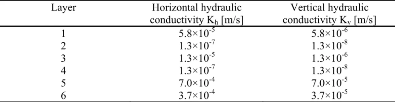
(6) 3.2 Grid A six-layered grid of 104 rows and 112 columns is constructed. The dimensions of a basic cell are 100 m x 100 m. The grid is gradually refined to cells with a dimension of 50 by 50 m near the pumping wells. The dimensions of the cells don't exceed 1.5 times the dimensions of their neighboring cells. For numerical reasons, the length-width-ratio of a cell doesn't exceed 10.. 3.3 Hydraulic conductivity Hydraulic conductivity values for the different layers of the study area are derived from pumping tests, discharge versus drawdown data and grain size distributions. The pumping tests are recovery tests analyzed with Theis and Jacob's recovery equation for confined aquifers (Kruseman et al. 1991). Twelve recovery tests were carried out in layer 1, three tests in layer 5 and eleven tests in layer 6. Discharge versus drawdown data were analyzed using the Thiem-Dupuit equation for steady-state flow (Kruseman et al. 1991). Thirteen analyses were carried out for layer 1, one for layer 3, one for layer 5 and 22 for layer 6. Grain size distributions of six samples of layer 6 were available. They were analyzed with the Beyer formula and the Zamarin formula (Kasenow 2002), two empirical methods to relate grain size to hydraulic conductivity. No hydraulic conductivity measurement was carried out in layers 2 and 4. Hydraulic conductivity values for these layers are therefore taken from a previous groundwater study in the study area. Average values of all hydraulic conductivity measurements were calculated for each layer. In horizontally layered sediments, horizontal hydraulic conductivity is larger than vertical hydraulic conductivity. Therefore it is assumed that the ratio of Kh to Kv equals 10 (Table 2). Layers 5 and 6 are clearly the most permeable aquifers of the Pleistocene. Layers 2 and 4 are the least permeable layers. They form a natural barrier for downward ground water flow. These average hydraulic conductivity values will be used as a first estimation of the hydraulic conductivity of each layer and will be optimized during the calibration of the ground water flow model.. 6.

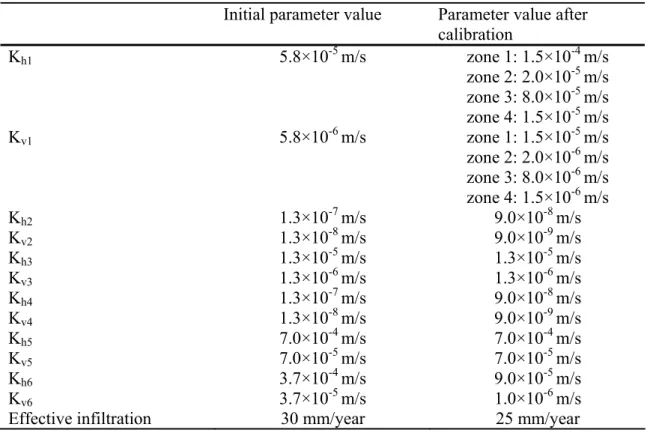
(7) Table 2 3.4 Calibration Measured groundwater levels from 32 piezometers -17 in the Upper Pleistocene (layer1) and 15 in the Lower Pleistocene (layer 6) - are available for calibration. The model is calibrated in steady-state conditions. Hydraulic conductivity and recharge were changed by "trial and error" calibration and by automatic calibration using PEST. Figure 2 shows the calculated versus observed piezometric heads for layer 1 and 6 before calibration. For layer 1, the dots are quite symmetrically distributed around the bisector. The absolute mean error is 1.16 m. In layer 6, the calculated piezometric head is larger than the measured piezometric head for all measuring points except one. The absolute mean error of this layer is 0.95 m.. Figure 2 Figure 3 shows the calculated versus observed piezometric heads for layer 1 and 6 after trial and error calibration. The mean absolute error of layer 6 diminished from 0.95 m to 0.39 m. The dots are now much better centered around the bisector than before calibration. Layer 1 is divided into 4 different zones with different hydraulic conductivities based on the geological well logs. The absolute mean error of layer 1 has decreased from 1.16 m to 0.70 m. The parameter that changed the most is hydraulic conductivity of layer 6 (Table 3). The horizontal conductivity of layer 6 was divided by 4; the vertical hydraulic conductivity was divided by 36. As a result, the ratio of Kh/Kv of layer 6 no longer equals 10 but 90. This large Kh/Kv-ratio can be interpreted considering the geologic build up of this layer. This layer consists of thick coarse sand to gravel layers divided by thin clay layers. The thick gravely layers result in a high horizontal hydraulic conductivity, whereas the thin clay layers lower the vertical hydraulic conductivity. Calibration also resulted in choosing lower hydraulic conductivities for the two clayey layers, layer 2 and layer 4. The hydraulic conductivities of these layers were divided by 1.5. 7.

(8) Figure 3 Table 3 The automatic calibration is executed by PEST, which is a parameter estimation routine. PEST minimizes the sum of the squared residuals, using the Gauss-Marquardt-Levenberg algorithm. Two restrictions are imposed. The first restriction is that in every layer the hydraulic conductivity in the x-direction has to stay the same as the hydraulic conductivity in the y-direction. In other words, the hydraulic conductivity is the same in every horizontal direction. The second restriction is that a minimum and a maximum value of every parameter are chosen. The lower bound is the initial value divided by 10, the upper bound is the initial value multiplied by 10. The automatic parameter estimation procedure results in the same mean absolute errors as the trial-and-error calibration. In this case, automatic calibration does not succeed in lowering these errors.. 3.5 Results The calculated piezometric east-west profile (Fig. 4) shows that in layer 1, on the west side of the river, the groundwater flows to the river. On the east side of the river there is no considerable groundwater flow. Between layer 1 and layer 5 and 6 there is a limited downward vertical groundwater flow. In layer 6, the pumping wells play an important role in the groundwater flow.. Figure 4 The calculated steady-state water balance (Fig. 5) provides an understanding of the interaction between the different layers of the area, the river, infiltration, the pumping wells and the fluxes at the boundaries. In layer 1, the water input comes mainly from fluxes across side boundaries. Infiltration also provides 17 % of the water input. The river is responsible for the largest water output. Other water outputs are fluxes across side boundaries and a flux of 8208 m³/day from layer 1 to layer 2. Layer 2 is a clayey layer 8.

(9) with no flux side boundaries. The vertical flux coming from layer 1 passes entirely to layer 3. Layer 3 is a thin sand layer, through which almost the entire flux coming from layer 2 flows to layer 4. There is only a small difference between the water input across side boundaries and the water output across side boundaries. Layer 4 is again a clayey layer with no flux side boundaries. The vertical flux coming from layer 3 goes entirely to layer 5. The water inputs of layer 5 are fluxes across side boundaries and the vertical flux coming from layer 4. The main outputs are fluxes across side boundaries and a vertical flux towards layer 6. The pumping wells of layer 5 are also responsible for a small water output. Layer 6 has a water input of 4218 m³/day coming from fluxes across side boundaries and a water input of 5252 m³/day coming from layer 5. The most important water outputs are the pumping wells, extracting 6181 m³/day. This means that a part of the water extracted in the pumping wells has to come from downward vertical fluxes. The influx across the side boundaries alone cannot provide 6181 m³/day.. Figure 5 4. Transport simulation Simulation of transport in the studied region is carried out using two different approaches: forward particle tracking using MODPATH (Pollock 1994) and transport simulation using MT3D (Zheng and Wang 1999) including transport by advection and dispersion.. 4.1 Boundary conditions At the boundaries of the transport model, the concentration gradient, and hence the dispersive flux, is assumed zero. In the three main pollution sources, i.e. the municipal waste disposal site, the sewage oxidation pond and the sewage treatment plant, no information about the concentrations of the different pollutants is available. Therefore, a constant arbitrary concentration of 1000 is applied.. 9.

(10) 4.2 Transport parameters The main input properties of the layers are the effective porosity and the longitudinal and transverse dispersivities. The effective porosity is set to a uniform value of 0.10, based on former studies and literature values in similar conditions (Anderson and Woesner 1996). Determination of the values of the dispersivities is somewhat more complex. Values of dispersivity are dependent on the scale of testing or observation (Zheng and Bennett 1995). The scales or cell dimensions used in this transport model are 50 m and 100 m. For a cell dimension of 50 m the longitudinal dispersivity according to Gelhar et al. (1992) is approximately 0.3 m, for a cell dimension of 100 m the longitudinal dispersivity according is approximately 5 m. As simplification, a longitudinal dispersivity of 5 m is adjudged to the whole area. As a rule of thumb, and in the absence of site specific data, horizontal transverse dispersivity can be taken about one order of magnitude smaller than longitudinal dispersivity, while vertical transverse dispersivity can be taken about two orders of magnitude smaller (Zheng and Bennett 1995). For this transport model this means that the horizontal transverse dispersivity is 0.5 m, while the vertical transverse dispersivity is 0.05 m.. 4.3 Results Figure 6 shows a map with computed MODPATH path lines 10 years after particle release. Figure 7 shows an east-west profile with computed MODPATH path lines 18 years after particle release. The particles do not seem to migrate to large depths, but travel nearly horizontally to the river. The deepest simulated particle reached a depth of only 11 m. According to these computations, the first particles that reach the river are particles coming from the sewage treatment plant. They reach the river after 10 years. The last particles that reach the river are particles coming from the municipal waste disposal site. They need 18 years to reach the river. The particles do not end up in the deep wells and do not seem to contaminate the drinking water.. Figure 6. 10.

(11) Figure 7 MT3D transport modeling shows that contaminants from the sewage treatment plant could reach the river after approximately 8 years. Contaminants coming from the sewage oxidation pond reach the river after about 9 years and contaminants coming from the municipal landfill reach the river after approximately 13 years. Concentrations at depths of 5, 15, 25 and 35 m below the main pollution sources were also calculated. The concentrations at a depth of 15 m below the main pollution sources are already several times smaller than the concentration at a depth of 5 m and the concentrations at a depth of 25 m and 35 m are negligibly small. The transport model thus confirms the results of forward particle tracking. At this stage of the investigation on the basis of the available data, it seems that the pollutants do not reach considerable depths and that the drinking water production wells of the Lower Pleistocene are therefore not threatened by these pollution sources.. 5. Sensitivity analysis In this study, several simplifications and assumptions about boundary conditions and parameter values were made because of limited data availability. This has of course consequences for the accuracy of the results and for the reliability of the main conclusion that the pollutants are no threat for the drinking water wells. To check whether this conclusion holds with somewhat different boundary conditions and parameter values, a sensitivity analysis and a worst case scenario analysis are carried out. First, the effects of boundary conditions, hydraulic conductivities, river parameters and infiltration on the downward vertical water fluxes from layer 1 to 2 and from layer 5 to 6 are examined. The vertical groundwater flow between the different layers probably plays an important role in the possible migration of dissolved contaminants to the Lower Pleistocene layers. The sensitivity to boundary conditions is shown in Figure 8. The water flux from layer 1 to layer 2 is very sensitive to all boundary conditions, especially those of layer 1, 5 and 6. Increasing the specified heads of layer 1 by 2 m results in a 24 11.

(12) % increase of the water flux from layer 1 to 2. Increasing the specified heads of layer 5 and 6 by 2 m causes a 24 % decrease of this groundwater flux. The water flux from layers 5 to layer 6 is dependent on the boundary conditions of layer 5 and 6. Lowering the specified heads at the boundaries of layers 5 and 6 by 2 m causes an 11% increase of the groundwater flux from layer 5 to 6. Increasing the boundary conditions of layer 5 and 6 by 2 m causes a decrease of 19 % of this groundwater flux. The sensitivities of the vertical fluxes to hydraulic conductivity, conductance and infiltration are shown in Figure 9. Both water fluxes are affected the most by changes in K2 and K4, the hydraulic conductivities of the clayey layers. Multiplying K2 by 10 increases the water flux from layer 1 to 2 with 135 %, multiplying K4 by 10 increases the water flux from layer 5 to 6 by 61 %.. Figure 8 Figure 9 Secondly, the sensitivities of computed travel times and concentrations to hydraulic conductivity of layer 1, effective porosity and dispersivity are examined. The following abbreviations are used: t1. travel time to the river of contaminants coming from the sewage treatment plant. t2. travel time to the river of contaminants coming from the sewage oxidation pond. t3. travel time to the river of contaminants coming from the municipal landfill. c1. contaminant concentration at a depth of 15 m below the sewage treatment plant. c2. contaminant concentration at a depth of 15 m below the sewage oxidation pond. c3. contaminant concentration at a depth of 15 m below the municipal landfill. Figure 10 shows the main results of these calculations. The travel times to the river decrease by increasing hydraulic conductivity, by decreasing effective porosity and by increasing dispersivity. Larger hydraulic conductivity values result in lower solute concentrations below the pollution sources since contaminants can flow more easily away horizontally from the pollution source if the porous medium is more permeable. Effective 12.

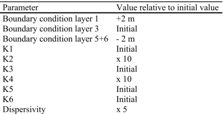
(13) porosity has no significant effect on the concentration distribution. Increasing dispersivity leads to larger concentrations below the pollution sources. Dispersion does not only include longitudinal dispersion but also, however to a smaller extent, transversal dispersion. This leads to a spreading of the contaminants transversally to the flow direction. Therefore the contaminants reach larger depths.. Figure 10 6. Worst case scenario analysis From the sensitivity analysis, the effect of most parameters on the downward migration of contaminants is known. A worst case scenario is built by giving every input parameter that value - from a range of possible or realistic values - that results in the largest and fastest downward migration of contaminants. Table 4 shows the worst case scenario parameter values. The prescribed piezometric heads at the boundaries of layer 1 are increased by 2 m. Further increasing these heads would be unrealistic, since this means that the water table would be higher than topography. The boundary conditions of layer 5 and 6 are lowered 2 m. This is a significant lowering since the total range of measured hydraulic heads in layers 5 and 6 is only 2 m. The hydraulic conductivities of the clay layers are multiplied by 10. This means that the horizontal and vertical hydraulic conductivities of these layers are now approximately 1×10-6 m/s and 1×10-7 m/s respectively. These values are high for sediments consisting mainly of clay and silt (Fetter, 2001) and are therefore appropriate worst case values. The overall longitudinal dispersivity is multiplied by 5, so that its value is now 25. All other input parameters and variables keep their initial values since they clearly have a less significant effect on the downward migration of contaminants.. Table 4 In this worst case scenario, the dissolved solutes still migrate to the river and not to the production wells in the Lower Pleistocene. The contaminants reach however greater. 13.

(14) depths: concentrations of 1/1000 of the constant concentration applied at the pollution sources are present up to 77 m depth, thereby penetrating a few meters in layer 2. This worst case scenario demonstrates that it is very unlikely that the contaminants coming from the sewage treatment plant, the sewage oxidation pond and the municipal waste disposal site could reach the drinking water wells of the Lower Pleistocene. The pollution sources are thus not situated in the capture zone of the production wells.. 7. Discussion and conclusion The main objective of this study was to determine whether the dissolved solutes coming from the municipal waste disposal site, the sewage treatment plant and the former sewage oxidation pond could reach the drinking water wells of the Lower Pleistocene in the study area. A groundwater flow and transport model was constructed and the results demonstrate that the wells would not be threatened by the pollution sources. The boundary conditions and parameter values of this model are however subject to large uncertainty, due to limited data availability. This results of course in large uncertainty of the results of the model. To build confidence in the conclusion of this study, a sensitivity analysis and a worst case scenario analysis were carried out. In the sensitivity analysis, the effect of boundary conditions and parameter values on the downward migration of pollutants was investigated. In the worst case scenario analysis, all variables and parameters were given the value - from a range of realistic values - that results in the largest downward migration of pollutants. Even in the worst case scenario, the contaminants from the pollution sources do not reach the drinking water wells. This study has shown that sensitivity analysis and worst case scenario analysis are efficient tools to deal with uncertainty in hydrogeological modeling and to build confidence in model results in cases with limited data availability.. References Anderson M, Woesner W (1992) Applied groundwater modeling - Simulation of flow and advective transport, Academic Press, New York. 14.

(15) Asante-Duah DK (1998) Risk Assesment in Environmental Management, John Wiley & Sons Ltd., Chichester, England Calow P (1998) Handbook of Environmental Risk Assessment and Management, Blackwell Science, Oxford, England Dou CH, Woldt W, Bogardi I, Dahab M (1995) Steady-state groundwater flow simulation with imprecise parameters. Water Resources Research 31(11): 2709-2719 Fetter CW (2001) Applied hydrogeology, Prentice Hall, New Jersey Gelhar LW, Welty C, Rehfeldt KW (1992) A critical review of data on field-scale dispersion in aquifers. Water Resources Research 28(7): 1955-1974 Kasenow M (2002) Determination of Hydraulic Conductivity from Grain Size Analysis, Water Resources Publications LLC, Highlands Ranch, Colorado Kruseman GP, De Ridder NA (1991) Analysis and evaluation of pumping test data, International Institute for Land Reclamation and Improvement, Wageningen, The Netherlands Levy J, Clayton MK, Chesters G (1998) Using an approximation of the three-point Gauss–Hermite quadrature formula for model prediction and quantification of uncertainty. Hydrogeology Journal 6(4): 457 - 468. Nauner K (2000) A sérülékeny földtani környezetben telepített Mátészalka Városi Vízmű v. zbázisanak vizsgálata,. Miskolci Egyetem, Miskolc, Hungary (In Hungarian) Pollock DW (1994) User's Guide for MODPATH/MODPATHPLOT, Version 3: a particle tracking post-processing package for MODFLOW, the U.S. Geological Survey finite-difference ground-water flow model. USGS Open-File Report 94-464, USGS, Reston, Virginia Thornthwaite CW (1948) An approach towards a rational classification of climate. Geographical Review 38(1): 55-94 ÜnlÜ K, Parker JC, Chong PK (1995) Comparison Of Three Uncertainty-Analysis Methods To Assess Impacts On Groundwater Of Constituents Leached From Land-Disposed Waste. Hydrogeology Journal 3(2): 4-18 Zheng C, Wang P (1999) MT3DMS: a modular three-dimensional multispecies transport model for simulation of advection, dispersion, and chemical reactions of contaminants in groundwater, US Army Corps of Engineers, Tuscaloosa Zheng C , Bennett GD (1995) Applied contaminant transport modelling - theory and practice, Van Nostrand Reinholds, New York. 15.

(16) Tables Table 1 Description of the 6 hydrostratigraphical units of the Pleistocene. Layer 1. Average thickness 65 m. Layer 2. 25 m. Layer 3 Layer 4. 7m 40 m. Layer 5. 20 m. Layer 6. 100 m. Description Thin layers of sand, silt and clay Clay or clayey sand with thin sand layers Sand Clay or clayey sand with thin sand layers Heterogeneous unit consisting of coarse sand and gravel layers alternating with clay layers Thick coarse sand and gravel layers alternating with thin clay layers. Upper Pleistocene Middle Pleistocene. Lower Pleistocene. 16.

(17) Table 2 Average measured values of the hydraulic conductivities of each layer. Layer 1 2 3 4 5 6. Horizontal hydraulic conductivity Kh [m/s] 5.8×10-5 1.3×10-7 1.3×10-5 1.3×10-7 7.0×10-4 3.7×10-4. Vertical hydraulic conductivity Kv [m/s] 5.8×10-6 1.3×10-8 1.3×10-6 1.3×10-8 7.0×10-5 3.7×10-5. 17.

(18) Table 3 Parameter values before and after trial-and-error calibration. Initial parameter value Kh1. 5.8×10-5 m/s. Kv1. 5.8×10-6 m/s. Kh2 Kv2 Kh3 Kv3 Kh4 Kv4 Kh5 Kv5 Kh6 Kv6 Effective infiltration. 1.3×10-7 m/s 1.3×10-8 m/s 1.3×10-5 m/s 1.3×10-6 m/s 1.3×10-7 m/s 1.3×10-8 m/s 7.0×10-4 m/s 7.0×10-5 m/s 3.7×10-4 m/s 3.7×10-5 m/s 30 mm/year. Parameter value after calibration zone 1: 1.5×10-4 m/s zone 2: 2.0×10-5 m/s zone 3: 8.0×10-5 m/s zone 4: 1.5×10-5 m/s zone 1: 1.5×10-5 m/s zone 2: 2.0×10-6 m/s zone 3: 8.0×10-6 m/s zone 4: 1.5×10-6 m/s 9.0×10-8 m/s 9.0×10-9 m/s 1.3×10-5 m/s 1.3×10-6 m/s 9.0×10-8 m/s 9.0×10-9 m/s 7.0×10-4 m/s 7.0×10-5 m/s 9.0×10-5 m/s 1.0×10-6 m/s 25 mm/year. 18.

(19) Table 4 Worst case scenario parameter values. Parameter Boundary condition layer 1 Boundary condition layer 3 Boundary condition layer 5+6 K1 K2 K3 K4 K5 K6 Dispersivity. Value relative to initial value +2 m Initial -2m Initial x 10 Initial x 10 Initial Initial x5. 19.

(20) Figure captions Fig. 1 East-west profile thought the study area, showing the six hydrostratigraphical units Fig. 2 Calculated versus observed heads of layers 1 and 6 before calibration Fig. 3 Calculated versus observed heads of layers 1 and 6 after calibration Fig. 4 Calculated piezometric W-E profile. Vertical exaggeration = 30. Maximum velocity = 4.7×10-6 m/s = 40.6 cm/day Fig. 5 Calculated water balance of the study area [m³/day] Fig. 6 Piezometric map with pathlines 10 years after particle release Fig. 7 Piezometric east-west profile with pathlines 18 years after particle release Fig. 8 Sensitivity of vertical water fluxes to boundary condition changes Fig. 9 Sensitivity of vertical water fluxes to hydraulic conductivities (K), river conductancy (C) and infiltration (I) Fig. 10 Sensitivities of travel times and concentrations to the hydraulic conductivity of layer 1, the effective porosity and the dispersivity. 20.

(21) Figures. 21.

(22) 22.

(23) 23.

(24) 24.

(25) 25.

(26) 26.

(27) 27.

(28) 28.

(29) 29.

(30) 30.

(31)