LES of knocking in engines using dual heat transfer and two-step reduced schemes

O

pen

A

rchive

T

OULOUSE

A

rchive

O

uverte (

OATAO

)

OATAO is an open access repository that collects the work of Toulouse researchers and

makes it freely available over the web where possible.

This is an author-deposited version published in : http://oatao.univ-toulouse.fr/

Eprints ID : 14489

To link to this article : DOI:10.1016/j.combustflame.2015.07.023

URL : http://dx.doi.org/10.1016/j.combustflame.2015.07.023

To cite this version : Misdariis, Antony and Vermorel, Olivier and

Poinsot, Thierry LES of knocking in engines using dual heat transfer

and two-step reduced schemes. (2015) Combustion and Flame, vol.

162 (n° 11). pp. 4304-4312. ISSN 00102180

Any correspondance concerning this service should be sent to the repository

administrator: [email protected]

LES of knocking in engines using dual heat transfer and two-step

reduced schemes

Antony Misdariis

_{, Olivier Vermorel}

_{, Thierry Poinsot}

b_{CERFACS, CFD Team, 42 Avenue G. Coriolis, 31057 Toulouse Cedex 01, France}

c_{Institut de Mécanique des Fluides de Toulouse, CNRS, Avenue C. Soula, 31400 Toulouse, France}

Keywords:

LES Knock Autoignition

Internal combustion engine Heat transfert

a b s t r a c t

Large Eddy Simulation of knocking in piston engines requires high-fidelity physical models and numerical techniques. The need to capture temperature fields with high precision to predict autoignition is an addi-tional critical constraint compared to existing LES in engines. The present work presents advances for LES of knocking in two fields: (1) a Conjugate Heat Transfer (CHT) technique is implemented to compute the flow within the engine over successive cycles with LES together with the temperature field within the cylinder head walls and the valves and (2) a reduced two-step scheme is used to predict both propagating premixed flames as well as autoignition times over a wide range of equivalence ratios, pressures and temperatures. The paper focuses on CHT which is critical for knocking because the gas temperature field is controlled by the wall temperature field and knocking is sensitive to small temperature changes. The CHT LES is compared to classical LES where the temperatures of the head and the valves are supposed to be homogeneous and im-posed empirically. Results show that the skin temperature field (which is a result of the CHT LES while it is a user input for classical LES) is complex and controls knocking events. While the results of the CHT LES are obviously better because they suppress a large part of the empirical specification of the wall temperatures, this study also reveals a difficult and crucial element of the CHT approach: the description of exhaust valves cooling which are in contact with the engine head for part of the cycle and not in the rest of the cycle, leading to difficulties for heat transfer descriptions between valves and head. The CHT method is successfully applied to an engine studied at IFP Energies Nouvelles where knocking characteristics have been studied over a wide range of conditions.

1. Introduction

To increase the efficiency of reciprocating engines, downsizing has become a new standard in the automotive industry[1]. By combin-ing smaller cylinder sizes with turbo-chargers, engines can be oper-ated in a region of higher efficiency. For moderate downsizing lev-els, this technique enables to decrease fuel consumption significantly and thus pollutants emissions. However abnormal combustions pre-vent engine manufacturers from using advanced levels of downsiz-ing. Abnormal combustion results from the competition between the turbulent propagation of the premixed flame initiated by the spark plug and the spontaneous ignition of the fresh gas. When high pres-sure and high temperature are encountered in the fresh gas in front of the flame front (also called end-gas), the auto-ignition delay drops

∗ _{Corresponding author at: CERFACS, CFD Team, 42 Avenue G. Coriolis, 31057}

Toulouse Cedex 01, France.

E-mail address:[email protected](A. Misdariis).

and can become lower than the time needed by the premixed flame to burn the charge. This kind of auto-ignition events leads to abnor-mal combustions such as knocking or rumble and can destroy the en-gine. Over the last decades, the increase of engines compression ra-tios lead to the same issues[2,3]and a better understanding of heat transfer and engine cooling allowed to control knocking. Nowadays, such fluid/solid interactions remain a key-parameter but it is not sufficient to control abnormal combustions in highly downsized en-gines. Increasing the engine resistance to knocking requires a better understanding of these phenomena. Although optical diagnostics are not easy to perform, existing experimental studies[4–6]highlighted some key features leading to abnormal combustions: (1) the intensity of knock is linked to the portion of fresh gas when auto-ignition oc-curs[7]and (2) detonation waves may appear in knocking cycles. The basic mechanism leading to detonation in such flows was studied by Zeldovich[8]who showed that a 1D temperature gradient in a flow close to auto-ignition could initiate a detonation wave. This mecha-nism was studied later by Bradley et al.[9]or Clavin et al.[10]and

Table 1

Properties of the materials used in the CHT simulation. Symbol Cast iron steel

Density [kgm−3_{] ρ 2675 7500}

Heat capacity [J/(kg K)] Cp 900 450

Heat conductivity [W/(m K)] λ 100 36

has become the prototype configuration used to illustrate how deto-nation can begin in an engine. Even though detodeto-nation can hardly be observed directly inside a piston engine several studies were carried-out in canonical configurations[8,11]suggesting that conditions were indeed favorable to detonation in knocking engines.

In this context, Large Eddy Simulations (LES) can provide detailed information to analyze abnormal combustion. Peters et al.[12]used simulations to identify regions where a Deflagration to Detonation Transition (DDT) can occur based on cold flow LES results and on the Zeldovich et al. theory. Robert et al.[13]proved that LES can be used to evaluate the knocking tendency of an experimental engine. They retrieved quantitatively the experimental behavior of the real engine and performed a first analysis of abnormal combustion thanks to LES. Obviously temperature plays a major role for knock and in a real engine the temperature field is expected to control knocking events to a large extent. For instance, wall heat transfer dictates the tem-perature level at Top Dead Center (TDC) when ignition is performed just before knock can begin near hot regions. This issue becomes even more important for engines running with abnormal combus-tion where local and intermittent hot spots found near high tem-perature walls can initiate auto-ignition inside fresh gases. In that sense, the use of realistic wall temperatures is of first importance when studying abnormal combustions with numerical simulations. The potential benefits of conjugate heat transfer simulations for pis-ton engines flows are pointed out in[14]and the same methodol-ogy is used in[15]. These studies proved that abnormal combustion events are influenced by wall temperatures and that Conjugate Heat Transfer (CHT) must be accounted for in these simulations, even in the context of RANS simulations. Here, the impact of CHT on knocking is investigated using individual cycles computed with LES. The draw-back of this method is that hundreds of cycles would be needed to account for cycle to cycle variabilities and obtain converged statistics, thus implying large CPU cost and simulation times. In this context, re-cent LES work[16–18]proved that, with a limited number of cycles, LES can predict cyclic variations. More recently, it was also shown that LES can provide detailed informations on knocking with a few engine cycles only[13]. The scope of the present paper is to improve abnormal combustion LES by including a comprehensive description of conjugate heat transfer with LES.

2. Configuration and methodology

In an engine, conjugate heat transfer controls wall temperatures and has a strong impact on combustion[19] because of the long residence time of the fresh gas in the cylinder prior to combustion triggered around TDC. The large variations of the combustion cham-ber volume and thus of the thermodynamic conditions promote heat exchanges at the boundaries and impact the combustion process. The wall temperatures used in numerical simulations are usually ob-tained from experimental measurements or from a priori estimations. This approach can provide an appropriate global behavior but local information is missing. In particular, the sophisticated cooling system used for the cylinder head can lead to temperature in-homogeneities that can have an impact on abnormal combustion. Only one hot wall zone can be enough to trigger knocking. This situation differs from ‘classical’ LES in engines, far from knocking conditions where wall temperatures play a more limited role[20–22]. In this paper,

First guess of wall temperatures

Spatial distribution of mean heat fluxes LES simulation of a

few engine cycles Solid Heat Transfer simulation New set of skin

temperatures No Yes Converged CHT results Converged heat fluxes ?

Fig. 1. Diagram of the weak coupling algorithm to perform a CHT simulation.

conjugate heat transfer is solved by means of a fully coupled simu-lation between fluid and solid so that relevant boundary conditions can be used to study knocking. While such studies have already been performed using RANS[15], they require much more care in a true LES framework as described in the next section.

2.1. Coupling methodology

In order to use realistic boundary conditions, a common strategy consists in using two different solvers: one for LES and another one to solve the heat equation in the solid domain. In such simulations, the characteristic time of the heat conduction in the solid

τ

(with L the solid characteristic length and Dsthe solid diffusivity) is

often several orders of magnitude higher than the combustion char-acteristic time

τ

δ

δ

speed). For instance, assuming a valve head of L= 10 mm and with the properties of steel (Table 1), the conduction characteristic time is:

τ

λ

(ρ

)

(

)

while for an iso-octane/air flame at 40 bar and 700 K, the combustion characteristic time is:

τ

δ

1.10−4

1.0 = 1.10−4s (2)

For this particular case, the conduction characteristic time is five or-ders of magnitude bigger than the conduction characteristic time: the solid acts like a low-pass filter and only sees a mean heat flux coming from the fluid domain. A numerical difficulty directly introduced by this time scales difference is that the convergence speeds differs in the fluid and in the solid domains. The convergence for the solid tem-perature is too long to be computed with LES. In practice however, this time scales difference can be exploited efficiently by recogniz-ing that only a weak couplrecogniz-ing between the two domains is sufficient. Decoupling the computations of LES in the cylinder and temperature in the solid walls allows to reach a converged state at the fluid/solid interface by only considering a mean averaged field of heat fluxes as inputs for the heat transfer simulation in the solid. The method-ology used to obtain the converged conjugated heat transfer at the fluid/solid interface is based on such a weak coupling (Fig. 1). The two solvers are run sequentially: first, an initial set of wall skin tem-peratures is obtained from experimental measurements or from 0D

Fig. 2. Comparison of 1D stoichiometric isooctane/air laminar flame speed with

com-plex chemistry[36], the standard two-step chemistry and the IPRS model.

simulations[23]. This set of wall temperature is used to compute the fluid dynamics thanks to the LES solver and wall Heat Fluxes (HF) are locally integrated over the full engine cycle. Then, the Heat Transfer (HT) solver is used to compute the steady temperature field inside the solid domain. Finally, the converged temperature at the fluid/solid in-terface is used to update the wall temperature field of the LES simu-lation. This coupling loop is performed until convergence of the heat fluxes and temperature at the interface.

2.2. Numerical set-up

In the present work, the fully compressible explicit code (called AVBP) is used to solve the filtered multi-species 3D Navier–Stokes equations with realistic thermochemistry on unstructured meshes

[24,25]. Based on the ESO2approach[26], numerics is handled with

the second-order accurate in space and time Lax–Wendroff scheme

[27]and a Two-step Taylor–Galerkin finite element scheme (TTG), third-order accurate in space and time[28]for phases which require increased accuracy (compression and combustion). The Smagorinsky sub-grid scale model is used[29]and boundary conditions use the NSCBC approach[30]. A simple 2-step scheme chemistry is used and sub-grid scale combustion is accounted for with the Thickened Flame for LES (TFLES) model since it has been successfully tested in numer-ous configurations outside piston engines[31–34]as well as in pis-ton engines[16,17]. Auto-ignition delays predictions is ensured by the Ignition to Propagation Reduced Scheme (IPRS) model[35]. The main idea of this model is that the pre-exponential constant A of the first reaction (fuel oxidation) takes different values at low and high temperatures. The low-temperature value of A controls the autoigni-tion time while the high-temperature value controls the flame speed. With this formalism, the low-temperature constant AAIis replaced by

a function of the fresh gas conditions, adjusted to predict the auto-ignition delay over a wide range of pressures and temperatures while the high-temperature value Apropensures the right flame speeds over

the same temperature and pressure range as shown in[35]. Note that this model predict the auto-ignition delay only and is not able to reproduce the cold flame phenomena.Figures 2and3show the sults obtained with IPRS in 1D laminar flames and homogeneous re-actors for operating conditions corresponding to the ones observed in the engine studied in the present paper. The Energy Deposition (ED) model[37]is used for spark ignition and moving meshes are han-dled with the ALE formalism[38]. Because of the high values of the Reynolds numbers, resolution of thermal and aerodynamic bound-ary layers would require very refined meshes at walls and would lead to unaffordable CPU cost when dealing with complex configurations. This issue is even more critical in IC engine simulations when using moving meshes: the mesh displacement would introduce a large de-formation of the smallest mesh elements that would lead to numeri-cal errors. Here wall functions were used[21,32,39,40].

The energy equation inside the solid domain is solved by the AVTP solver [41]. Spatial discretization is handled with a second-order

Fig. 3. Comparison of AI delays obtained with a 2-step chemistry and a reference

chemistry[36]in an homogeneous reactor.

Solid Heat transfer simulation – 67 hCPU

67 ms

60s

LES – 20000 hCPU

T

CHT iteration 1

Fig. 4. Schematic of the Conjugated Heat Transfer (CHT) simulation.

Galerkin scheme[42]and temporal integration uses a first-order for-ward implicit scheme. The resolution of the implicit system is done with a parallel matrix free conjugate gradient method [43]. Heat fluxes are determined by means of a Fourier’s law and tempera-ture dependent heat conductivity coefficients and heat capacities are used.

As shown inFig. 4, the LES simulation for one cycle represents 67 ms of physical time (for an engine speed of 1800 rpm) while 60 s of physical time is needed to reach steady state inside the solid. How-ever, thanks to the use of an implicit time marching, the heat transfer simulation inside the solid uses large time-steps and the final cost is negligible compared to the LES simulation. Eventually, the cost of the CHT simulation is only due to the extra LES simulations performed at each CHT iteration to reach a converged temperature field at the fluid/solid interface.

2.3. Experimental configuration and operating point

The target configuration is an experimental mono-cylinder 4 valves turbo-charged ECOSURAL engine shown inFig. 5. This engine is installed at IFP Energies Nouvelles in the framework of the french ANR (Research National Agency) ICAMDAC project to study abnor-mal combustion in downsized spark-ignited engines. The spatial dis-cretization uses full tetrahedral meshes for the fluid and solid do-mains. The fluid domain begins in the inlet plenum and finishes on the outlet plenum, a procedure which has been shown to provide the required accuracy for LES by specifying boundary conditions far away from the cylinder[17,21]. The mesh size for the fluid domain

Inlet plenum Outlet plenum Intermediate plenum Combustion chamber

Fig. 5. Sketch of the experimental Ecosural engine test bench.

Table 2

Main engine specifications. Crank Angle Degrees (CAD) are relative to combustion top dead cen-ter. IVO and IVC respectively stand for Inlet Valve Opening and Closure while EVO and EVC stand for Exhaust Valve Opening and Closure.

Compression ratio [-] 10.64

Bore [mm] 77.0

Stroke [mm] 85.8

Connecting rod length [mm] 132.2

IVO/IVC [CAD] 353/-162

EVO/EVC [CAD] 142.5/-352.5

varies between 2.2 and 12 million cells while a fixed 1.7 million cells mesh is used for the solid domain. As shown inFig. 6, the mesh at the fluid/solid interface is the same between the two domains. Two metals are accounted for in the CHT solver: the cylinder head is made of cast iron while steel is used for valves. The properties of cast iron and steel are summarized inTable 1.

The engine geometrical specifications (Table 2) and the operating point described inTable 3correspond to the knocking conditions. For this regime, the dynamics of the flow predicted by LES were validated against PIV measurements[44].

3. Conjugate heat transfer simulation

All LES of piston engines require the specification of the wall tem-peratures. In the present work, two methods were used to obtain these quantities:

Table 3

Definition of the operating point chosed in the ICAMDAC database to study the knocking phenomena. IMEP stands for In-dicated Mean Effective Pressure.

Engine rotation speed [rpm] 1800

IMEP [bar] 19.0

Intake pressure [bar] 1.8 Intake temperature [K] 308

Fuel [-] C8H18

Table 4

Skin wall temperatures obtained from 0D simulations used for the empirical simulation[13].

Patch Temperature [K]

Cylinder head 409 Intake valves 639 Exhaust valves 784

• The usual method is to assume that (1) the chamber walls can be decomposed in isothermal elements: piston head, intake, exhaust valves and (2) the temperature of these elements is known, usu-ally obtained either through a global energy balance or through empiric evaluations (this method is called empirical here). • The CHT method where heat transfer in the walls (cylinder head

and valves) is coupled to LES to obtain the skin wall temperature by a fully coupled simulation (called CHT here).

Note that in the empirical approach, the elements temperatures are often tuned to match experimental observations (volumetric effi-ciency, heat losses, etc.). Here we use the wall temperatures proposed for the same engine by Robert et al.[13](Table 4). For the CHT ap-proach, walls temperatures are a result of the computation and not an input data.

During one cycle the diffusion through the cylinder head and valves is actually not steady because of moving parts, of the unsteadi-ness of fluid dynamics and of the intermittency of combustion. For in-stance, for an engine cycle of 720 CA, the heat flux to the exhaust valve is high during combustion and exhaust phases while it is low during the intake stroke because of the low temperature of the fresh gases. In practice, however, because of the difference in characteristic times between heat diffusion inside the solid and flow motion in the cylin-der, the solid acts as a low-pass filter and receives a heat flux coming from the fluid domain which can be averaged over the whole engine cycle, allowing to decouple LES and heat transfer codes. The most sig-nificant complexity for the CHT method is the description of the dif-fusive heat fluxes between valves and cylinder head. When valves are closed, heat can diffuse from the valve to the cylinder head depending

Spark plug

cooling system

cylinder head

intake valve exhaust valve Fig. 6. Illustration of a typical mesh for the LES simulation (left) and for the CHT simulation (right).

Fig. 7. Heat fluxes through the cylinder head during 15 consecutive cycles.

Fig. 8. Mean heat flux between the cylinder head and the fluid integrated over each

engine cycle.

on the heat resistance of the contact zones between valves and cylin-der head which is controlled by the force of the valve spring[45]. On the other hand in the open position, no thermal exchange can occur between the valve seat and the cylinder head. This geometry change has proved to be a major difficulty for the CHT approach because it controls the exhaust valve temperature and therefore the onset of knocking. The first part of this paper (Section 3.1) assumes that dur-ing the whole engine cycle, valves remain in the closed position as far as heat fluxes in the engine walls in concerned. This assumption clearly over-estimates the exhaust valve cooling and leads to lower temperatures. This problem is addressed inSection 3.4.

3.1. Heat transfer cycle-to-cycle variability

In spark ignited piston engines RMS pressures due to cycle-to-cycle variability can reach several percents of the mean in-cylinder pressure. Cycle to cycle variability can also affect heat fluxes through the walls. In order to evaluate the variability of heat fluxes,Fig. 7

shows the value of the total flux to the cylinder head (valves are not included) obtained from LES for 15 consecutive engine cycles with the empirical approach and reveals a significant variability. For en-gine cycles where the whole mixture is burned quickly, pressure and temperature in the cylinder are high and increase thermal exchanges at the boundaries leading to large and variable fluxes during the com-bustion phase. However,Fig. 7also shows that the main flux from the fluid to the cylinder head occurs during the exhaust stroke when the cylinder is filled with hot gases and high velocities caused by the ex-haust valve opening. For this engine, all the fuel is consumed when the exhaust valves open, so that the temperature inside the cylinder is almost the same for all cycles. Even though the instantaneous flux to the cylinder head varies from cycle to cycle (Fig. 7), its value av-eraged over each cycle exhibits much less variation (Fig. 8). To eval-uate the impact of these variations on combustion, the engine cycle

a.

b.

Fig. 9. Converged temperature on the solid skin after the first CHT iteration. (a) Engine

cycle with the highest mean heat transfer and (b) engine cycle with the lowest heat transfer.

showing the highest heat fluxes and the engine cycle with the low-est heat fluxes were used as boundary conditions for a HT simula-tion inside the solid domain. The converged solusimula-tion on the skin at the interface between fluid and solid domains is displayed inFig. 9

for those two engine cycles. Even though these two cycles repre-sent extreme scenarios in terms of fluid-solid heat fluxes, these HT simulations show that the impact on the solid temperature is very low. The mean temperature integrated over the cylinder head and valves is 441 K for the engine cycle with the highest heat fluxes while it is equal to 438 K for the engine cycle with the lowest heat fluxes. As expected, the highest temperatures are found on the ex-haust valves but they vary only from 607 K for the low flux cycle

Fig. 10. Convergence of the mean temperature and heat fluxes at the interface

be-tween the fluid and solid domains.

to 611 K for the high flux cycle. In other words, temperature in the solid is mainly driven by heat exchanges with the ambient air and coolant fluid and its sensitivity to variations of the heat flux com-ing from the fluid domain is low. This shows that the temperature field in the engine walls is almost insensitive to the details of each cycle and can be computed using the cycle averaged heat fluxes. Note that for the two simulations performed, steady state is reached after about 60 s of physical time meaning that a synchronized coupling be-tween fluid and solid domains is actually out of reach for this kind of applications.

3.2. CHT convergence and influence on the fluid solution.

Figure 10shows the evolution of the mean solid temperature and the mean heat fluxes integrated over the cylinder head and valves us-ing the algorithm ofFig. 1. Convergence is reached very quickly: at the end of the second CHT iteration, the error compared to the fourth CHT iteration on the mean heat flux is 0.2% and 0.3% on the mean temper-ature.Figure 11shows the evolution of the skin temperature used as boundary condition for the LES. The quick convergence of the CHT simulation observed for global quantities inFig. 10is also observed for the local distribution of the wall temperature. The main advantage of using a CHT methodology is to provide the full wall temperature field while the empirical simulation relies on a user-specified mean temperature for each element of the model (cylinder head, valves). For a more quantitative comparison, temperature profiles on cylin-der head and valves (seeFig. 11b for profile positions) are plotted in

Fig. 12. These profiles prove that it is difficult to obtain good estima-tions of wall temperature with an empirical guess. Up to 60 K varia-tions of temperature are observed on the center of the cylinder head (A-line inFig. 12a). This is even worse for exhaust valves where the skin temperature at the exhaust valve center is 200 K higher than its surroundings (B-line inFig. 12b). The exhaust valve shaft only sees burned gases during the whole engine cycle. On the contrary, the valve tip is cooled down by the cylinder head. The resulting tem-perature profile in the valve can not be guessed using empirical ap-proaches and CHT is required to provide consistent temperature fields for LES.

3.3. Impact of CHT on combustion

In order to investigate the effect of using realistic wall tempera-tures, a first multi-cycle LES is performed with empirical wall tem-peratures. Then each individual cycle is re-played with different wall temperatures from CHT simulations.Table 5summarize the different cases.Figure 13shows the pressure evolution for 3 engine cycles with highing knock intensity in A-case and B-case. In both experiments and LES, knocking cycles are characterized by pressure oscillations: pres-sure records are used to determine the occurrence of knocking and its onset. For a fair comparison between experiments (where 500 cy-cles are captured) and LES (which only contains 15 cycy-cles) samples

a.

b.

Fig. 11. Convergence of the CHT simulation. (a) Converged solution in the solid after

the first CHT iteration and (b) converged solution after the fourth CHT iteration.

a.

b.

Fig. 12. Temperature profiles on cylinder head and exhaust valves for empirical and CHT. A-line (a) and B-line (b). The empirical profiles are specified by the user as

Fig. 13. Temporal evolution of the in-cylinder pressure recorded by a pressure probe

for 3 engine cycles with high knocking intensity. (a) Corresponds to A-case and (b) corresponds to B-case.

Table 5

Definition of LES cases. Spark timing is given with reference to TDC. Nucis a Nusselt Number that characterizes the contact between valves and cylinder head.

Case Spark timing [CAD] Wall temperature Nuc Knocking

A-case +6 Empirical – Yes

B-case +6 CHT 0.3 No

C-case +6 CHT 0.6 Yes

D-case 0 CHT 0.6 Yes

E-case −4 CHT 0.6 Yes

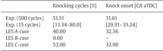
Table 6

Comparison of knocking statistics between experiments and LES. Knocking cycles [%] Knock onset [CA aTDC]

Exp. (500 cycles) 51.51 31.61

Exp. (15 cycles) [13.34–80.0] [29.91–35.24]

LES A-case 40.00 32.56

LES B-case 0.00 –

LES C-case 53.00 32.90

of 15 experimental cycles are used to compute the same statistics (Table 6). These statistics show that the numerical setup including TFLES and IPRS model for combustion modeling is able to reproduce the knocking behavior in the A-case. For the B-case simulation how-ever, no knocking cycles are observed. The cycles plotted are the same for the two cases. The combustion process differs between the two simulations even during the propagation of the flame but the most remarkable result is that in B-case, no oscillations representative of knocking are observed. The difference in the combustion process can be attributed to slight changes due to the different temperature of the walls. These skin temperature differences induce not only gas tem-perature differences but also flow modifications (Fig. 14): the com-bination of temperature and flow variations between A and B-Cases eventually leads to very different knocking results. Under the same operating conditions,[13]observed that auto-ignition of the end-gas mainly occurred near the hot exhaust valves. In the present results, the absence of knocking in B-case is indeed due to the lower exhaust valve temperature compared to A-case. In A-case, the exhaust valve temperature was set to 784K while it shows large local variations in the CHT simulation but does not exceed 620 K (Figs. 11and12).

Figure 15shows iso-surfaces of temperature at 780 K and 800 K for the same cycle as inFig. 14, 2 CAD after ignition for the empirical

(A-case) and the CHT (B-(A-case) LES. The distribution of hot spots clearly

differs between the two simulations and more particularly, the large hot spot observed above the hot exhaust valve in A-case disappears

Fig. 14. Aerodynamic field in a (⃗x, ⃗z) cut-plane and iso-surfaces of temperature 2 CAD

after ignition for A-case (a) and B-case (b). This cycle corresponds to the cycle with the highest knocking intensity for A-case.

Fig. 15. 780 K and 800 K temperature iso-surfaces 2 CAD after spark timing for the

cycle with highest knock intensity in A-case (a) and B-case (b). This cycle corresponds to the cycle with the highest knocking intensity.

Fig. 16. Illustration of the fictitious layer model to account for teat transfer between

cylinder head and valves.

in B-case. This zone corresponds to the location where auto-ignition eventually occurs in A-case explaining why B-case does not create knocking. This simulation shows that autoignition is extremely sensi-tive to local temperature properties: improving the boundary condi-tions (going from an empirical temperature field to a fully computed temperature field) on the engine walls is sufficient to inhibit knock-ing. This confirms that wall boundary conditions are crucial to predict knocking. Even if the CHT methodology provides a better description of wall temperatures, it actually degrades knocking predictions be-cause it lead to too low temperature of the exhaust valves. It suggests that the CHT approach used in this section must be improved. The next section shows that the most critical part of this method is the description of the contact between exhaust valves and cylinder head.

3.4. Improvement of the CHT model.

This section shows how to improve the CHT approach and capture knocking when it should occur. For the sake of simplicity, the model previously used for the CHT simulation assumed:

• A closed position of the valves during the whole cycle.

• No contact resistance between cylinder head and valves when valves are closed.

These assumptions have a major impact on heat fluxes between cylinder head and exhaust valves. The main problem is that assum-ing closed position and perfect contact between head and valves dur-ing the whole cycle over-predicts the cooldur-ing of the hot valves by the water-cooled cylinder head. The heat flux in this region actually fol-lows a cyclic evolution: it is high when the valve is closed and it is zero when the valve is open. The typical exhaust phase duration is 200 CAD which represents 28% of the whole cycle. Heat diffusion in-side the solid does not see the valve motion because of its high fre-quency but this motion has an impact on the mean fluxes through the cylinder head–valve interface. This section describes a simple im-provement technique to account for the reduced valve heat fluxes due to the period when valves are open and to the contact resistance be-tween the two parts. The flux

%

%

τ

Rc

(3) with

τ

to the cycle duration (

τ

cylin-der head and valves temperature and Rcis the contact resistance Rc

between head an valves.Eq. (3)suggests a simple method (called here fictitious layer) to account for the reduced heat flux due to con-tact resistance and valve opening without having to actually use a geometry where the valves move. A small ‘contact’ zone of thick-ness e (e= 0.3 mm here) and conductivity

λ

placed between valves and cylinder head. The conductivity

λ

Fig. 17. Convergence of the mean temperature and heat fluxes at the interface between

the fluid and solid domains with Nucontact= 0.6.

Fig. 18. Temperature field at the fluid/solid interface after the fourth CHT iteration.

can be chosen so that the heat flux through this layer

%

λ

(T

v)

for:

λ

τ

λ

con-ductivity of the valves to have:

λ

λ

τ

(4) where Nucis a contact Nusselt number. This allows to mimic the

ef-fect of valve opening on the valve temperature while still using a fixed geometry. Nucis difficult to evaluate and remains an input for

the simulation. In the following (C-case, D-case and E-case) it is set to

Nuc= 0.6. For B-case where the layer of thickness e was supposed to

be made of steel, Nucis equal to

τ

The convergence of this modified CHT simulation is displayed

Fig. 17. As in the previous case, a steady state in terms of mean tem-perature and mean heat flux is obtained after the second CHT itera-tion.Figure 18shows the spatial distribution of temperature after the fourth CHT iteration. Compared to the B-case simulation (Fig. 11b) higher temperatures are observed. The temperature of the exhaust valve center increases from 605 K to 690 K. It is interesting to see that, once one tries to compute wall temperatures with precision, de-tails become important: the present results show that assuming that valves remain closed all the time leads to under predicted wall tem-peratures and, as shown above, to underestimated knocking. Correct-ing this problem with the model ofFig. 16andEq. (4)is sufficient to capture knocking cycles again: for a third multi-cycle simulation called C-case, 53% of knocking cycles are found with a mean onset at 32.9 CAD which matches experimental results (Fig. 19).

Finally, the same wall temperatures (from C-case) are kept to com-pute D-case and E-case with variable spark timing.Figure 20shows the evolution of the local pressure for three knocking cycles with high knocking intensity. The global trends from[13]are retrieved. When the spark timing is reduced, higher pressure levels are observed

Fig. 19. Temporal evolution of the in-cylinder pressure recorded by a pressure probe

in C-case(15 cycles).

LES C-case LES D-case LES E-case

Fig. 20. Temporal evolution of the in-cylinder pressure for 3 cycle with high knocking

intensity for C-case, D-case and E-case.

inside the cylinder. Auto-ignition occurs sooner in the cycle and knocking intensity is increased.

These simulations show that wall temperatures have a direct im-pact on the flow motion and on the combustion process. Especially when dealing with abnormal combustions, the auto-ignition delay can vary dramatically as a function of the local temperature condi-tions and an accurate prediction of the thermal boundary condicondi-tions is necessary. Even though the proposed model including a CHT simu-lation still uses some assumptions such as the definition of a contact Nusselt number, it replaces a complete field of uncertainties (the wall temperature field) by only one input (the contact Nusselt number). This permits to obtain local distributions of temperature that should be close to the physical behavior and compatible with LES precision.

4. Conclusions

In order to increase the precision of LES of knocking in piston en-gines, this paper focuses on a strategy that permits to access to a real-istic wall temperature field in the combustion chamber. The proposed methodology relies on a full Conjugate Heat Transfer (CHT) simu-lation between cylinder head, valves and the combustion chamber which provides all wall temperatures. These temperatures control the engine behavior, especially in terms of knocking showing the impor-tance of this input for precise LES. The second part of this paper ad-dresses the issue of heat transfer between cylinder head and moving valves. A simple methodology is proposed to account for this moving geometry and contact resistance in this region. LES performed in this paper show a strong impact of heat transfer and skin wall tempera-tures on the knocking behavior of the engine. The use of a CHT simu-lation instead of a priori defined, constant wall temperatures changes the distribution of hot spots that are likely to auto-ignite. This clear improvement of the LES strategy allows to provide more physical, meaningful data but results show that it also bring a new complex-ity: to model the valves temperatures (which control the knock on-set), the heat resistance between valve and head must be correctly

modeled and introduced in the CHT model, something which is not fully available today.

Acknowledgments

This work was granted access to the HPC resources of CCRT un-der allocations x20142b5031 made by GENCI (Grand Equipement Na-tional de Calcul Intensif) and PRACE (Partnership for Advance Com-puting in Europe) project N2013091887 SolitonCycLES. The authors acknowledge the financial support by the French ANR under grant ANR-10-VPTT-0002 ICAMDAC.

References

[1]G.T. Kalghatgi, SAE Trans. J. Fuels Lubr. 105 (1995).

[2]K.M. Chun, J.B. Heywood, SAE Paper (1989).

[3]T. Litzinger, Prog. Energy Combust. Sci. 16 (1990) 155–167.

[4]G.A. Ball, Proc. Combust. Inst. 5 (1955) 366–372.

[5]N. Kawahara, E. Tomita, Y. Sakata, Proc. Combust. Inst. 31 (2007) 2999–3006.

[6]M. Kanti, N. Kawahara, E. Tomita, Proc. World Hydrogen Energy Combust. 78 (2010) 141–148.

[7] K. Chun, J. Heywood, J. Keck, Proc. Combust. Inst. 22 (1989) 455–463, doi:10.1016/S0082-0784(89)80052-9.

[8]Y.B. Zeldovich, Combust. Flame 39 (1980) 211–214.

[9]D. Bradley, G.T. Kalghatgi, Combust. Flame 156 (2009) 2307–2318.

[10] P. Clavin, L. He, J. Fluid Mech. 306 (1996) 353–378, doi:10.1017/ S0022112096001334.

[11]K. Fieweger, R. Blumenthal, G. Adomeit, Combust. Flame 109 (1997) 599–619.

[12]N. Peters, B. Kerschgens, G. Paczko, SAE Paper (2012).

[13] A. Robert, S. Richard, O. Colin, L. Martinez, L.D. Francqueville, Proc. Combust. Inst. 35 (2015) 2941–2948, doi:10.1016/j.proci.2014.05.154.

[14]Y. Li, S. Kong, Int. J. Heat Mass Transf. 54 (2011) 2467–2478.

[15]D. Linse, A. Kleemann, C. Hasse, Combust. Flame 161 (2014) 997–1014.

[16]B. Enaux, V. Granet, O. Vermorel, C. Lacour, L. Thobois, V. Dugué, T. Poinsot, Flow Turbul. Combust. 86 (2011) 153–177.

[17]V. Granet, O. Vermorel, C. Lacour, B. Enaux, V. Dugué, T. Poinsot, Combust. Flame 159 (2012) 1562–1575.

[18]D. Goryntsev, A. Sadiki, M. Klein, J. Janicka, Proc. Combust. Inst. 32 (2009) 2759– 2766.

[19]A.H. Lefebvre, Gas Turbines Combustion, Taylor & Francis, 1999.

[20]S. Richard, O. Colin, O. Vermorel, A. Benkenida, C. Angelberger, D. Veynante, Proc. Combust. Inst. 31 (2007) 3059–3066.

[21]B. Enaux, V. Granet, O. Vermorel, C. Lacour, C. Pera, C. Angelberger, T. Poinsot, Proc. Combust. Inst. 33 (2011) 3115–3122.

[22]V. Granet, O. Vermorel, T. Leonard, L. Gicquel, T. Poinsot, AIAA J. 48 (2010) 2348– 2364.

[23]C. Pera, C. Angelberger, SAE Paper (2011).

[24]T. Schønfeld, T. Poinsot, in: Annual Research Briefs, Center for Turbulence Re-search, NASA Ames/Stanford Univ., 1999, pp. 73–84.

[25]L.Y.M. Gicquel, G. Staffelbach, T. Poinsot, Prog. Energy Combust. Sci. 38 (2012) 782–817.

[26] A. Misdariis, A. Robert, O. Vermorel, S. Richard, T. Poinsot, Oil Gas Sci. Technol. Rev. IFP Energ. Nouv. 69 (2014) 83–105, doi:10.2516/ogst/2013121.

[27]P.D. Lax, B. Wendroff, Com. Pure App. Math. 17 (1964) 381–398.

[28]O. Colin, M. Rudgyard, J. Comput. Phys. 162 (2000) 338–371.

[29]J. Smagorinsky, Mon. Weather Rev. 91 (1963) 99–164.

[30] T. Poinsot, S. Lele, J. Comput. Phys. 101 (1992) 104–129, doi: 10.1016/0021-9991(92)90046-2.

[31]P. Quillatre, O. Vermorel, T. Poinsot, P. Ricoux, Ind. Eng. Chem. Res. 52 (2013) 11414–11423.

[32]P. Schmitt, T. Poinsot, B. Schuermans, K.P. Geigle, J. Fluid Mech. 570 (2007) 17–46.

[33]G. Kuenne, A. Ketelheun, J. Janicka, Combust. Flame 158 (2011) 1750–1767.

[34]L. Gicquel, G. Staffelbach, T. Poinsot, Prog. Energy Combust. Sci. 38 (2012) 782– 817.

[35]A. Misdariis, O. Vermorel, T. Poinsot, Proc. Combust. Inst. 35 (2015) 3001–3008.

[36]S. Jerzembeck, N. Peters, P. Pepiot-Desjardins, H. Pitsch, Combust. Flame 156 (2009) 292–301.

[37]G. Lacaze, E. Richardson, T.J. Poinsot, Combust. Flame 156 (2009) 1993–2009.

[38]C.W. Hirt, A. Amsden, J.L. Cook, J. Comput. Phys. 131 (1974) 371–385.

[39] O. Cabrit, F. Nicoud, Phys. Fluids 21 (2009) 055108, doi:10.1063/1.3123528.

[40]O. Vermorel, S. Richard, O. Colin, C. Angelberger, A. Benkenida, D. Veynante, Com-bust. Flame 156 (2009) 1525–1541.

[41]F. Duchaine, N. Maheu, V. Moureau, G. Balarac, S. Morea, Journal of Turbomachin-ery 136 (2013) 051015.

[42]J. Donea, A. Huerta, Finite Element Methods for Flow Problems, John Wiley & Sons, 2003.

[43] V. Frayssé, L. Giraud, S. Gratton, J. Langou, ACM Trans. Math. Softw. 31 (2005) 228–238, doi:10.1145/1067967.1067970.

[44]A. Robert, Simulation Aux Grandes Echelles Des Combustions Anormales Dans Les Moteurs Downsizés à Allumage Commandé, INP Toulouse, 2014 (Ph.D. thesis).

[45]Y. Aabdel-Fattah, The Mechanics of Valves Cooling in Internal-Combustion En-gines: Investigation into the Effect of Valve-Seat Inserts on the Heat Flow from Valves towards the Cooling Jacket, University of Bradford, 2009 (Ph.D. thesis).