En vue de l'obtention du
DOCTORAT DE L'UNIVERSITÉ DE TOULOUSE
Délivré par :Institut National Polytechnique de Toulouse (INP Toulouse)
Discipline ou spécialité :
Dynamique des fluides
Présentée et soutenue par :
M. NADIM ZGHEIB
le vendredi 13 mars 2015
Titre :
Unité de recherche : Ecole doctorale :
DYNAMIQUE DES COURANTS DE GRAVITE NON-AXISYMETRIQUES
Mécanique, Energétique, Génie civil, Procédés (MEGeP)
Institut de Mécanique des Fluides de Toulouse (I.M.F.T.)
Directeur(s) de Thèse : M. OLIVIER EIFF
M. SIVARAMAKRISHNAN BALACHANDAR Rapporteurs :
M. ANDREW OOI, UNIVERSITE DE MELBOURNE M. TIAN-JAN HSU, UNIVERSITY OF DELAWARE
Membre(s) du jury :
1 M. OLIVIER THUAL, INP TOULOUSE, Président
2 M. ALEXANDRU SHEREMET, UNIVERSITE DE FLORIDE, Membre 2 M. SIVARAMAKRISHNAN BALACHANDAR, UNIVERSITE DE FLORIDE, Membre
RESUME
Les courants de gravité, écoulements issus de la présence d’un contraste de densité dans un fluide ou de la présence de fluides de densités différentes, sont rencontrés dans de nombreuses situations naturelles ou industrielles. Quelques
exemples de courants de gravité sont les avalanches, les marées noires et les courants de turbidité. Certains courants de gravité peuvent représenter un danger pour l’homme ou l’environnement, il est donc nécessaire de comprendre et de prédire leur dynamique. Cette thèse a pour objectif d’étudier l’évolution de courants de gravité de masse fixée, et notamment l’influence d’une forme initiale non-axisymétrique sur la dynamique, effet jusque-là peu abordé dans la littérature. Pour cela, une large gamme de paramètres est couverte, incluant le rapport de masse volumique entre le fluide ambiant et le fluide dans le courant, le rapport de forme initiale, la forme de la section horizontale de la colonne de fluide (circulaire, rectangulaire ou en forme de croix), le nombre de
Reynolds (couvrant jusqu’à 4 ordres de grandeur) et la nature du fluide lourd (salin ou chargé en particules). Deux campagnes d’expériences ont été menées et complétées par des simulations numériques hautement résolues. Le résultat majeur est que la propagation du courant et le dépôt de particules (lorsque particules il y a) sont fortement influencés par la forme initiale de la colonne de fluide. Dans le cas de la colonne
initialement rectangulaire le courant se propage plus vite et dépose plus de particules dans la direction initialement de plus courte dimension. Ce comportement
non-axisymétrique est observé dans une large gamme des paramètres étudiés ici. Pourtant les modèles analytiques existants et notamment le modèle dit de boîte (box model) qui prédit avec succès le comportement des courants de gravité/turbidité dans les cas plan et axisymétrique ne sont pas capables de reproduire ce phénomène. C’est pourquoi
une extension du box model a été développée ici, et est en mesure de décrire la
dynamique de courants de gravité de masse fixée dont la forme initiale est arbitraire. Le cas plus général d'un courant de gravité évoluant sur un plan incliné a été abordé et une dynamique intéressante a été observée.
ABSTRACT
Gravity currents are buoyancy driven flows that appear in a variety of situations in nature as well as industrial applications. Typical examples include avalanches, oil spills, and turbidity currents. Most naturally occurring gravity currents are catastrophic in nature, and therefore there is a need to understand how these currents advance, the speeds they can attain, and the range they might cover. This dissertation will focus on the short and long term evolution of gravity currents initiated from a finite release. In particular, we will focus attention to hitherto unaddressed effect of the initial shape on the dynamics of gravity currents. A range of parameters is considered, which include the density ratio between the current and the ambient (heavy, light, and Boussinesq currents), the initial height aspect ratio (height/radius), different initial cross-sectional geometries (circular, rectangular, plus-shaped), a wide range of Reynolds numbers covering 4 orders of magnitude, as well as conservative scalar and non-conservative (particle-driven) currents. A large number of experiments have been conducted with the abovementioned parameters, some of these experiments were complemented with highly-resolved direct numerical simulations. The major outcome is that the shape of the spreading current, the speed of propagation, and the final deposition profile (for particle-driven currents) are significantly influenced by the initial geometry, displaying
substantial azimuthal variation. Especially for the rectangular cases, the current propagates farther and deposits more particles along the initial minor axis of the rectangular cross section. This behavior pertaining to non-axisymmetric release is robust, in the sense that it is observed for the aforementioned range of parameters, but nonetheless cannot be predicted by current theoretical models such as the box model, which has been proven to work in the context of planar and axisymmetric releases. To
that end, we put forth a simple analytical model (an extension to the classical box model), well suited for accurately capturing the evolution of finite volume gravity current releases with arbitrary initial shapes. We further investigate the dynamics of a gravity current resulting from a finite volume release on a sloping boundary where we observe some surprising features.
5
REMERCIEMENTS
I would like to start by thanking my parents for their never-ending love and support and for providing me with the best education I could ask for. I am thankful for my sister’s guidance and grateful for my brother for being a great role model and making it possible for me to attend grad school.
It has been a wonderful journey. I had the pleasure and privilege of working with two great advisors, Prof. Balachandar and Prof. Bonometti, on some very interesting projects. Whether at University of Florida (UF) or Institut de Mécanique des Fluides de Toulouse (IMFT), they have been very generous with their time.
I am grateful to the joint PhD committee members for their constructive feedback. I would like to express my gratitude to Prof. O. Thual for making sure the PhD defense went as smoothly as possible at IMFT. I would like to express my thanks to Professors, H. Fan, D. Legendre, A. Sheremet, and L. Ukeiley for fruitful interactions following my PhD proposal. I am grateful to Prof. A. Ooi for a productive collaboration that resulted in an additional chapter to my thesis. I would like to acknowledge Prof. T. Hsu for his in-depth remarks of the thesis.
I was fortunate to be part of a dynamic and supportive group while at UF and IMFT. I would like to express my thanks to Mrugesh Shringarpure for his invaluable help with the spectral code. I would also like to acknowledge Georges Akiki, Subramanian Annamalai, Yue “Stanley” Ling, and Manoj Parmar for fruitful discussions and help with various topics.
I would like to express my sincere gratitude to Sébastien Cazin for help in setting up the experiments at IMFT and spending significant time to get me up to speed on post-processing. I would like to express my thanks to Hervé Ayroles for his assistance
6
during my 2014 visit to IMFT. I would like to acknowledge the members of group OTE, specifically Serge Font and Sylvain Belliot for their valuable day to day support with the experimental setup. I am deeply grateful to Sylvie Senny for her help during all the visits to IMFT. I would like to express my appreciation to Laurent Lacaze and Matthieu
Mercier for their valuable ideas and advice in the various aspects of the experiments. I am grateful to Cécile Molles for her help in sieving the particles.
Finally I would like to acknowledge funding support from the UF Graduate School and PIRE NSF, as well as IMFT, INPT, and the French Embassy in Miami (for the Chateaubriand Fellowship) for support while at IMFT.
7 SOMMAIRE
1 INTRODUCTION ... 10
1.1 Classification of Gravity Currents ... 11
1.1.1 Finite vs Continuous Release ... 11
1.1.2 Source of Current-Ambient Density Difference ... 11
1.1.4 Geometric Constraints ... 13
1.2 Classical Approaches ... 14
1.2.1 Laboratory Experiments ... 14
1.2.2 Numerical Simulations ... 15
1.2.3 Theoretical Models ... 15
1.3 Present Interest and Contributions ... 16
2 METHODOLOGY ... 25
2.1 Experiments ... 25
2.1.1 Setup ... 25
2.1.2 Measurements ... 27
2.1.3 Image Processing ... 29
2.2 Direct Numerical Simulations ... 30
2.3 Extended Box Model ... 32
2.3.1 Initial Condition ... 35
2.3.2 Time Integration and Spatial Discretization ... 37
3 LONG-LASTING EFFECT OF INITIAL CONFIGURATION IN GRAVITATIONAL SPREADING OF MATERIAL FRONTS ... 46
3.1 Background ... 46
3.2 Non-Circular Spreading of Density Currents ... 47
3.3 A New Model for the Prediction of the Propagation of Non-Circular Density Flows ... 53
3.4 Summary and Discussion ... 56
4 DIRECT NUMERICAL SIMULATION OF CYLINDRICAL PARTICLE-LADEN GRAVITY CURRENTS ... 66
4.1 Background ... 66
4.2 Mathematical Formulation ... 69
4.3 Results ... 71
4.3.1 Three-Dimensional Structures ... 71
4.3.2 One-Dimensional Time Evolution ... 73
4.3.2 Front Location ... 73
4.3.3 Deposition ... 74
4.3.4 Wall Shear-Stress and Near-Wall Dynamics ... 76
8
5 DYNAMICS OF NON-CIRCULAR FINITE RELEASE GRAVITY CURRENTS ... 87
5.1 Background ... 87
5.2 Experimental and Numerical Procedures ... 92
5.2.1 Experimental Setup ... 92
5.2.2 Preliminary Verifications ... 94
5.2.3 Numerical Procedure ... 96
5.3 High-Reynolds Number Boussinesq Density Currents ... 97
5.3.1 Self-Similarity of the Front Contour of Non-Circular / Non-Planar Gravity Currents ... 98
5.3.2 Local Front Froude Number of Non-Circular / Non-Planar Gravity Currents ... 101
5.4 Extended Box Model Simulations ... 104
5.4.1 Equations and Assumptions ... 104
5.4.2 Examination of the Extended Box Model ... 106
5.4.3 A Scaling Law for the Final Shape of Non-Circular Gravity Currents... 109
5.5 Discussion ... 111
5.5.1 Varying Current-to-Ambient Density Ratio ... 112
5.5.2 Turbidity Current ... 112
5.5.3 Effect of Wall Friction ... 113
5.5.4 Influence of the Reynolds Number ... 113
5.5.5 Varying the Vertical and Horizontal Aspect Ratios ... 114
5.5.6 Possible Influence of the Initial Curvature and the Local Instantaneous Curvature ... 115
5.5.7 Vortical Structures of Non-Circular / Non-Planar Gravity Currents ... 116
5.6 Summary and Discussions ... 118
6 PROPAGATION & DEPOSITION OF NON-CIRCULAR FINITE RELEASE PARTICLE-LADEN CURRENTS ... 137
6.1 Background ... 137
6.2 Experiments of Finite-Release Non-Circular Particle-Laden Currents ... 140
6.2.1 Experimental Setup ... 140
6.2.2 Procedure ... 141
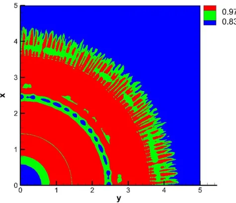
6.2.3 Results ... 143
6.2.3.1 Evolution in the horizontal (x,y)-plane ... 143
6.2.3.2 Evolution along the x- and y-axes ... 146
6.2.3.3 Influence of the settling velocity ... 148
6.2.3.4 Influence of the settling velocity ... 149
6.2.3.4 Influence of the initial height aspect ratio ... 149
6.2.3.4 Influence of the lateral boundaries ... 150
6.3 Simulations of Finite-Release Non-Circular Particle-Laden Currents ... 151
6.3.1 Equations and Numerical Setup ... 151
6.3.1 Front Evolution ... 153
6.3.3 Particle Deposition... 156
6.3.4 Possible Contribution of Bedload Transport ... 158
9
6.3.5 Vortex Dynamics ... 161
6.4 Conclusion ... 162
7 INVESTIGATION OF FINITE RELEASE GRAVITY CURRENT ON A UNIFORM SLOPE ... 180
7.1 Background ... 180
7.2 Theory and Laboratory Experiments ... 183
7.3 Direct Numerical Simulations of Circular Gravity Currents on an Incline ... 184
7.3.1 Numerical Model ... 184
7.3.2 Initial Condition ... 186
7.4 Structure ... 187
7.5 Front Velocity ... 190
7.6 Mass Redistribution ... 195
7.6.1 Spanwise and Streamwise Average ... 195
7.6.2 Instantaneous Velocity Field ... 196
7.7 Internal Circulation and Froude Number ... 198
7.8 Head and Entrainment ... 200
7.8.1 Defining the Head of the Gravity Current ... 201
7.8.2 Properties of the Head ... 202
7.8.2.1 Geometric Properties and Total Buoyancy ... 202
7.8.2.2 Comparisons with Thermal Theory and Experiments... 204
7.9 Reynolds Number Dependence ... 205
7.10 Conclusion ... 206
8 CONCLUSIONS AND FUTURE WORK ... 238
APPENDIX: NUMERICAL DETAILS OF THE EXTENDED BOX MODEL ... 244
10 CHAPTER 1 INTRODUCTION
When two fluids of different densities are placed in contact with one another such that the contact interface is parallel to the gravitational field, a predominantly horizontal flow develops (as a result of the hydrostatic pressure difference at the interface) in which the denser of the two fluids (termed heavy fluid) intrudes into its less dense neighbor (termed light fluid) in a ground hugging manner (Figure 1-1). This buoyancy driven flow is termed a gravity current (or density current) and forms the subject of the present thesis.
There are numerous natural flows that fall under the above description, and some of these flows are very common that they have been assigned simplified and perhaps more appropriate labels such as sand storms, avalanches, and oil spills (to name a few). In an attempt to simplify and gain a better understanding of their
dynamics, gravity currents have been divided into different categories. These categories may depend on a variety of parameters, which include the type of release, the source of the density difference (the driving force), the extent of the density difference (or density ratio), the geometric confinement or restrictions, etc. Section 1.1 will provide a brief summary for some of these categories of relevant interest to this thesis. Section 1.2 will then elaborate on some of the classical experimental, numerical, and theoretical
approaches to this problem. Finally, section 1.3 will discuss the present interests and contributions to the field of gravity currents.
11
1.1 Classification of Gravity Currents 1.1.1 Finite vs Continuous Release
A finite release gravity current (Simpson 1972, Huppert & Simpson1980, Bonnecaze et al. 1995, Hacker et al. 1996, Gladstone et al. 1998, Shin et al. 2004, Cantero et al. 2007a) corresponds to a scenario where a fixed volume of fluid is suddenly discharged into an ambient environment of different density whereas a continuous release (Garcia and Parker 1993, Hogg et al. 2005, Sequeiros et al. 2009, Shringarpure et al. 2012) usually originates from a large reservoir with a time-dependent flux 𝑞 of the form 𝑞 = 𝑞𝑠𝑡𝑠 where 𝑞𝑠 is a positive constant, 𝑡 stands for time and 𝑠 is an
exponent either positive (waxing release), negative (waning release), or null (fixed finite-volume release). A finite release is generally observed when the sides of a container suddenly collapse releasing the embodied fluid instantaneously, whereas a continuous release can result from a small rupture along one of the edges of a large container or a pipeline leading to a continuous discharge of material.
1.1.2 Source of Current-Ambient Density Difference
The density difference between the two fluids may arise as a consequence of temperature, concentration, or compositional (different fluids altogether) variations, or as a result of suspended of particles. The latter type is termed a particle-laden current (Bonnecaze et al. 1993, Hallworth & Huppert 1998, Gladstone et al. 1998, Necker et al. 2002) since the presence of particles gives rise to the excess density and hence the buoyancy driving source. In the case of temperature differences, one may think of a layer of cold (relatively heavy) air sweeping the bottom of a room occupied by warm (relatively light) air. Similarly, when fresh water (relatively light) from a river exits into the ocean (relatively heavy salty water), it flows along the surface, partially due to the
12
difference in salinity between fresh and salty water. On the other hand, a turbid mixture spreading on the seafloor constitutes an example where the excess density in the current also comes about from the suspension of sediments. The former two examples are homogeneous, scalar driven gravity currents, where the density of both fluids (in the absence of mixing between the current and the ambient fluid) remains unchanged. On the other hand, even in the absence of mixing, the density of a particle-laden current continues to evolve in space and time as a result of the continuous deposition of particles and possible reentrainment back into the flow (if the current is energetic enough).
1.1.3 Current to Ambient Density Ratio
The initial density jump across the interface need not be large, in fact less than a percent difference in density between both fluids is usually sufficient to drive a strong flow. The term Boussinesq flows is commonly used to denote those types of flows resulting from a small density difference between the fluids (Benjamin 1968, Rottman & Simpson 1983, Hartel et al. 2000, Marino et al. 2005, Ungarish & Zemach 2005). There are some key differences in the structure and shape of a gravity current depending on the initial density ratio between the heavy and light fluids. When the densities of both fluids are comparable, the advancing current senses the presence of the ambient, which imposes a significant resistive force on the intruding current. However, when the density of the current is much larger than that of the ambient (Birman et al. 2005, Etienne et al. 2005, Lowe et al. 2005, Ungarish 2007, Bonometti et al. 2008), as in the case of a dam break flow in which water spreads in air, the current does not sense nor perceives any resistance from the surrounding ambient (air in the present example). The presence or absence of a resistive force is manifested by the shape of the gravity current (Figure
13
1-2). A Boussinesq gravity current usually attains a slug-like shape with a “head” and a “body”, whereas the thickness of a non-Boussinesq current decreases monotonically as we approach the ambient fluid, reaching a minimum value at the front of the current. 1.1.4 Geometric Constraints
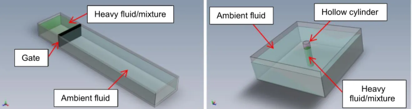
Gravity currents are usually studied in one of two canonical configurations, namely the planar and the axisymmetric setups (Figure 1-3). These configurations are popular and have been widely explored due to their simplicity. They may be easily constructed for experimental and numerical studies, and provide a more manageable challenge for modelling purposes (Shallow Water equations and Box Model). In the planar release case, a flat rectangular gate initially separates a rectangular reservoir of fluid from an ambient of different, usually smaller density. Similarly, at the start of the axisymmetric three-dimensional release, the current is confined inside a hollow circular cylinder at the centre of a large tank containing the ambient fluid (Huppert 1982,
Cantero et al. 2007), or in an expanding reservoir of relatively small angle of expansion, typically 10-15° (Huppert & Simpson 1980, Cantero et al. 2007a). The setups in Figure 1-3 correspond to a finite release scenario. For a continuous release, the gate would be partially lifted, and the trapped fluid would be continuously fed to maintain the desired volumetric discharge rate.
The planar setup may be thought of as a two-dimensional release since the current is confined to move along a specified direction, whereas for the circular release, the current would spread radially outwards (in all directions) but remain axisymmetric because of the initial circular nature of the release.
Gravity currents, when propagating horizontally into their ambient, usually undergo four main stages (Huppert & Simpson 1980). Initially when the current is
14
released, it accelerates from rest until it reaches a maximum velocity. During this highly transitional phase, termed the acceleration phase, the current undergoes rapid change in its velocity (zero to maximum), and the structure of the release also changes from mostly vertical to horizontal. This phase is often overlooked for three main reasons: (1) it is complex and transitional in nature, (2) it is relatively short lived, and (3) it is
presumed to have little effect on the long term dynamics of the current. Following the acceleration phase, the current reaches a steady-state phase referred to as the
slumping phase. During this phase, a planar (resp. cylindrical) current advances with a constant (resp. nearly constant) velocity and height (Gladstone 1998). At the end of the slumping phase, the current typically transitions to the inertial self-similar phase where the buoyancy driving force is balanced by the current’s inertia. During this phase, the current starts to decelerate as a consequence of its diminishing front height. Finally, as the current’s thickness continues to decrease, viscous and/or capillary forces become dominant, and the current evolves into the self-similar viscous/capillary phases.
1.2 Classical Approaches
The study of gravity currents is well developed with research spanning laboratory experiments, numerical simulations, and theoretical models.
1.2.1 Laboratory Experiments
Experiments constitute a very powerful and reliable approach to the study of gravity currents (for example Huppert & Simpson 1980, Bonnecaze et al. 1993, Marino
et al. 2005). Because of the relative ease and simplicity of conducting self-driven flows,
there has been hundreds of experiments reported to date on gravity currents. There are one or two popular quantities that are frequently monitored in experiments, namely the location of the front (from which the front velocity may be derived) and the thickness of
15
the current at various locations (head, body, tail). In the case of non-conserving currents (particle-laden flows), the final deposition pattern is typically measured as well.
Moreover, depending on the interest of the experimentalists, further specific quantities may be additionally monitored (thickness of the current, ambient entrainment, front instabilities, bottom erosion, etc.).
1.2.2 Numerical Simulations
Quantities such as ambient entrainment, bedload transport, and particle
resuspension are difficult and even costly to monitor experimentally. They might require additional resources such as high speed cameras, stress sensors, or relatively
expensive fluids. However, these aforementioned quantities, among others, may be calculated numerically with lesser effort and cost (for example Necker et al. 2002, Blanchette et al. 2005, Cantero et al. 2008). It is, in fact, for these hard to observe phenomena that numerical simulations become highly desirable. Fully resolved direct numerical simulations are very accurate but are limited to Reynolds numbers much smaller than what is realized in laboratory experiments and actual environmental or industrial gravity currents. Reynolds averaged and LES approaches have been used for investigating high Reynolds gravity currents (Ooi et al. 2007 Paik et al. 2009).
1.2.3 Theoretical Models
When numerical simulations become costly, or when fewer details about the flow are needed, researchers may decide to use simpler theoretical models to study gravity currents. These might range in complexity from algebraic equations such as the Box Model (Dade & Huppert 1995, Gladstone et al. 1998) to complicated sets of coupled partial differential equations with turbulence closure as well as entrainment and erosion models (such as the three and four equation models of Zeng & Lowe 1997 and Parker
16
et al. 1986). One of the most popular models, however is the one layer, inviscid shallow
water equations (Grundy 1986, Bonnecaze et al. 1995, Choi & Garcia 1995, Ungarish & Huppert 1998), which are derived from the Euler equations through scaling arguments and vertical integration.
1.3 Present Interest and Contributions
This thesis may be summarized by the following fundamental question: If we release a fixed volume of fluid into an ambient of different density, how would the initial shape of the release affect the dynamics of the flow? As we will shortly demonstrate, we find that the manner in which the fluid is released plays an important role in determining how the flow develops. On a horizontal plane the spreading current reaches a non-axisymmetric self-similar shape, whose aspect ratio depends on the shape of the initial release. On a sloping boundary, finite releases tend to evolve to an optimal self-similar shape, whose propagation speed could be substantially higher than for a corresponding planar current.
This dependence on the initial shape of release was first observed in our
experiments of saline, Boussinesq currents. We noticed (for non-axisymmetric releases) that regions close to the center of mass of the release advance farther and faster than regions far from the center of release. The difference in velocities along the front was significant, especially for rectangular cross-sections, where the layout of the rectangular release (beyond the self-similar inertial phase of spreading) would resemble an ellipse whose major axis coincided with that of the initial minor axis of the rectangular cross section.
This non-uniform spreading of material fronts is not limited to Boussinesq saline currents. It is of interest to know the influence of various parameters on this preferential
17
spreading. To that end, we performed a series of experiments and numerical
simulations in which we varied multiple parameters, one parameter at a time, to isolate their effect and contribution to this non-uniform flow. In these experiments, we examined the dependence on (1) the current-to-ambient density ratio by considering Boussinesq and non-Boussinesq currents, (2) the wall friction by investigating bottom (no-slip boundary condition) and top (no stress boundary condition) currents, (3) the shape (specifically the cross-section) of the release by considering circular, rectangular, and plus-shaped hollow cylinders, (4) the Reynolds number, which covered 4 orders of magnitude, (5) the local curvature of the release by using a right-angled rectangle and a rounded rectangle (in which the right angles are smoothened), (6) the height aspect ratio (ℎ𝑒𝑖𝑔ℎ𝑡/𝑟𝑎𝑑𝑖𝑢𝑠) of the release, which covered a range of [0.25,7], and (7) the presence of relatively heavy particles (particle-laden currents).
Based on the above experiments and simulations, we conclude that the
dependence on the initial shape holds for (i) heavy non-Boussinesq bottom currents, (ii) light surface currents, and (iii) particulate turbidity currents. The observed behavior is not influenced by wall friction and is independent of initial height aspect ratio. Only at very low Reynolds number we observe the current to spread to a near axisymmetric shape independent of initial release. Moreover, in the case of particle-laden currents, the final deposition profile of the particles displays substantial azimuthal variation, especially for the rectangular releases where the current deposits noticeably more particles along the initial minor axis of the rectangular cross section (compared with the initial major axis). We have performed a large number of experiments and
18
simple model to predict the counterintuitive spreading resulting from non-canonical initial releases.
Our simple model is based on the integral box model, which is classically used for predicting the evolution of gravity currents (Huppert & Simpson 1980). Despite the simplicity of the box model, it is able to reproduce the dynamics of axisymmetric and planar releases. However, straightforward application of the Box Model fails for non-axisymmetric releases. According to this model, the height remains uniform along the entire spreading patch, so the speed of propagation remains uniform along the current’s front during all the phases of spreading. Using the classical Box Model, an initially non-axisymmetric current inevitably becomes non-axisymmetric. Similarly, theories based on slumping and self-similar phases also fail to predict the sensitive dependence on the initial shape and the preferential propagation of non-axisymmetric gravity currents for the same reasons. Here, we propose an Extended Box Model based on partitioning of the initial release (into smaller sub-volumes) using geometric rays that are
perpendicular to the front. Once the various sub-volumes are obtained, the local fronts are advanced normal to themselves as in the Box Model. This initial partitioning is the key aspect of the present model, since it allows for non-uniform height and speed along the patch’s advancing front, during all the phases of spreading. This allows the model to capture the non-axisymmetric propagation of the front.
Unlike planar (two-dimensional) currents that are always unidirectional (do not admit a mean spanwise component of velocity), or axisymmetric currents that are ever diverging, circular releases on sloping boundaries may exhibit nearly unidirectional, diverging, or even converging phases of spreading. Of specific interest is the
19
converging phase of spreading, which leads to local peaks in buoyancy that translate into a second acceleration phase. Circular releases on sloping boundaries are thus significantly different than planar releases. The formation and evolution of gravity currents under such conditions are not well understood.
This thesis contains 7 chapters other than this introduction. The second chapter elaborates on the methodology, specifically the details behind the experimental and numerical setups as well as the proposed extended box model (EBM). The final chapter 8 will present conclusions and future work. The other 5 chapters are each self-contained and have already appeared as journal articles or will be submitted. They will be briefly described below.
Chapter 3: In this chapter we present results from laboratory experiments and fully-resolved simulations pertaining to finite release gravity currents with a non-axisymmetric cross-section. First, we demonstrate that, contrary to expectation, the effects of the initial shape influence the current’s evolution well into the self-similar phases. Then we identify the physical mechanisms responsible for this dependence and propose a new model capable of capturing the dynamics of such releases. Finally, we show that this dependence on initial configuration is robust for various types of gravity currents (homogeneous and inhomogeneous) over a wide range of parameters such as Reynolds number, density ratio, wall friction and aspect ratio, and discuss the
implications for the prediction of the propagation of natural gravity currents as oil spill, turbidity current and debris clouds. This chapter appeared in Theoretical &
20
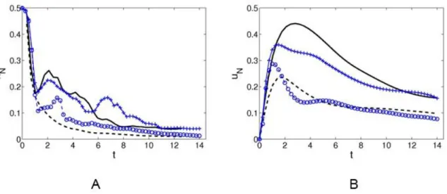
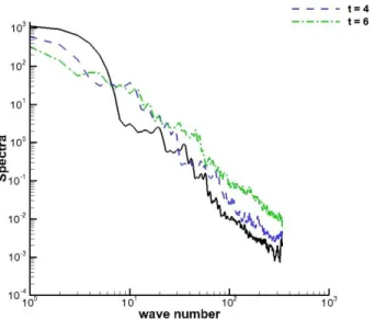
Chapter 4: We use highly resolved direct numerical simulations (DNS) to investigate axisymmetric particle-laden gravity currents. We consider the case of a full depth release with monodisperse particles at a dilute concentration where particle-particle interactions may be neglected. The disperse phase is treated as a continuum and a two-fluid formulation is adopted. We present results from two simulations at Reynolds numbers of 3450 and 10000. Our results are in good agreement with previously reported experiments and theoretical models. At early times in the simulations, we observe a set of rolled up vortices that advance at varying speeds. These Kelvin-Helmholtz (K-H) vortex tubes are generated at the surface and exhibit a counter-clockwise rotation. In addition to the K-H vortices, another set of clockwise rotating vortex tubes initiate at the bottom surface and play a major role in the near wall dynamics. These vortex structures have a strong influence on wall shear-stress and deposition pattern. Their relations are explored as well. This Chapter is currently under review for publication in Computers & Fluids.
Chapter 5: This chapter reports some new aspects of non-axisymmetric gravity currents obtained from laboratory experiments, fully resolved simulations and box models. Following the work of Chapter 3, where we demonstrated that gravity currents initiating from non-axisymmetric cross-sectional geometries do not become axisymmetric, nor do they retain their initial shape during the slumping and inertial phases of spreading, here we show that such non-axisymmetric currents eventually reach a self-similar regime during which (i) the local front propagation scales as t1/2 as in
circular releases and (ii) the non-axisymmetric front has a self-similar shape that
21
of non-Boussinesq, top-, and turbidity currents suggest that this dynamics is
independent of the density ratio, vertical aspect ratio, wall friction, and Reynolds number provided 𝑅𝑒 is large, 𝑅𝑒 ≥ 𝛰(104). The local instantaneous front Froude number
obtained from the fully-resolved simulations is compared to existing models of Froude functions. The recently reported extended box model capable of capturing the dynamics of such non-axisymmetric flows is used to propose a scaling law for the self-similar horizontal aspect ratio 𝜒∞ of the propagating front of a gravity current as a function of
the initial horizontal aspect ratio 𝜒0. The experimental and numerical results are in good
agreement with the proposed scaling law. This Chapter is currently under review for publication in Journal of Fluid Mechanics.
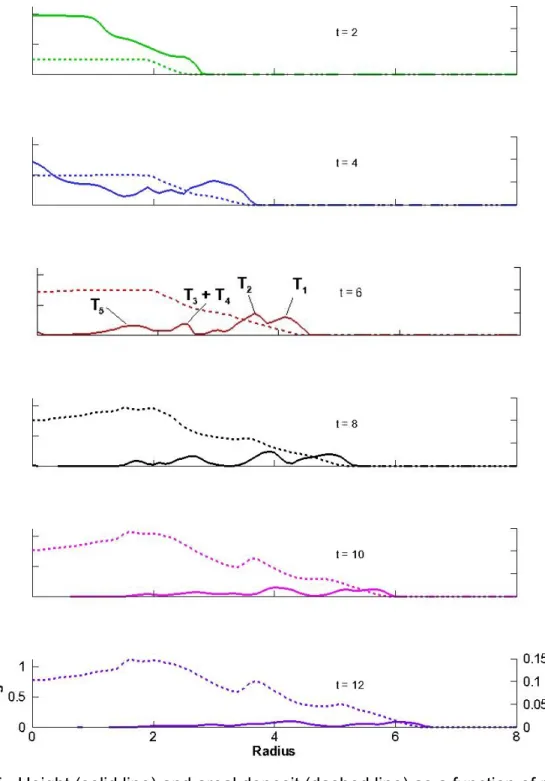
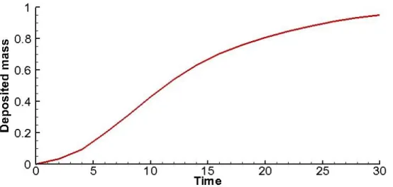
Chapter 6: The dynamics of non-axisymmetric turbidity currents is considered in this chapter. The study comprises a series of experiments and highly resolved simulations for which a finite volume of particle-laden solution is released into fresh water. A mixture of water and polystyrene particles of diameter 𝑑̃𝑝 = 300 μm and
density 𝜌̃𝑐 = 1012 kg/m3 is initially confined in a hollow cylinder at the centre of a large
tank filled with fresh water. Cylinders with two different cross sections are examined: a circle and a rounded rectangle in which the sharp corners are smoothened. The time evolution of the front is recorded as well as the spatial distribution of the thickness of the final deposit via the use of a laser triangulation technique. The dynamics of the front and final deposit are significantly influenced by the initial geometry, displaying substantial azimuthal variation especially for the rectangular case where the current extends farther and deposits more particles along the initial minor axis of the rectangular cross section. Several parameters are varied to assess the dependence on the settling velocity, initial
22
height aspect ratio, and volume fraction. Even though resuspension is not taken into account in our simulations, good agreement with experiments indicates that it does not play an important role in the front dynamics, in terms of velocity and extent of the current. However, wall shear stress measurements show that incipient motion of particles and particle reentrainment do occur in the body of the current and should be accounted for to properly capture the final deposition profile of particles. This Chapter is currently under review for publication in Physics of Fluids.
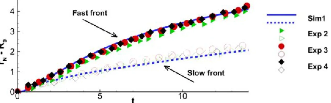
Chapter 7: In this chapter we report on the dynamics of circular finite-release Boussinesq gravity currents on a uniform slope. The study comprises a series of highly resolved direct numerical simulations for a range of bottom slopes between 5 and 20 degrees. Two Reynolds numbers are considered (𝑅𝑒 = 1000 and 𝑅𝑒 = 5000). The temporal evolution of the front is in excellent agreement with previous experiments. One of the most fascinating aspects of this study is the detection of a converging flow towards the centre of the domain. This converging flow is a result of the finite nature of the release coupled with the presence of a sloping boundary and leads to a second acceleration phase in the front velocity of the current. The second acceleration has never been reported in the context of gravity currents. Its significant implications on the short and long term behaviour on the current are discussed. These finite-release currents are invariably dominated by the head where most of the mixing and ambient entrainment occurs. We propose a simple method for defining the head of the current from which we extract various properties including the front Froude number and entrainment coefficient. The Froude number is seen to increase with steeper slopes,
23
whereas the entrainment coefficient is observed to be weakly dependent on the bottom slope. This Chapter will be submitted to Journal of Fluid Mechanics.
24
Figure 1-1. Conditions leading to the formation of a gravity current. At 𝑡𝑖𝑚𝑒 = 0, a hydrostatic pressure difference is present at the vertical interface. It increases linearly with depth, reaching a maximum at the bottom surface.
Figure 1-2. Schematic of a Boussinesq (top) and a non Boussinesq (bottom) current.
Figure 1-3. Canonical setups: Planar release (left), circular release (right).
Gra vit y Heavy Light 𝑡𝑖𝑚𝑒 = 0 𝑡𝑖𝑚𝑒 > 0 Heavy fluid/mixture Ambient fluid Gate Ambient fluid Heavy fluid/mixture Hollow cylinder
25 CHAPTER 2 METHODOLOGY
This chapter is arranged into three sections and provides details on the
experiments, numerical simulations, and the proposed extended box model. In section §2.1, we elaborate on the experimental setup and discuss how the experiments are performed. We specify the quantities of interest as well as the means of extracting and post-processing the data. Some of the experiments are complemented with direct numerical simulations using a spectral code that has been extensively verified (Cortese & Balachandar 1995, Cantero et al. 2007a). Details of the numerical simulations are presented in §2.2. Finally, we elaborate in §2.3 on the proposed extended box model. We present the governing equations and discuss some of the attributes of the model, including the initial partitioning and remapping of Lagrangian points.
2.1 Experiments
All experiments were performed at the Institut de Mécanique des Fluides de Toulouse (IMFT) at the experimental facilities of Ondes, Turbulence et Environnement (OTE) group. The details of the experiments are hereby presented.
2.1.1 Setup
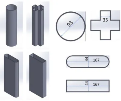
A schematic of the setup is shown in Figure 2-1. A hollow cylinder lies at the center of a square transparent tank. The cylinder traps within its walls a fluid or mixture (particles + water) with a different density (typically larger) than the ambient surrounding fluid, which predominantly consisted of tap water. Four cylinders were considered with different cross-sectional shapes: (i) circle (CS), (ii) plus shape (PS), (iii) rounded rectangle (RR), and a true rectangle (TR). The cylinders have roughly the same cross-sectional area (except for the TR, which has the same aspect ratio as that of the RR)
26
and are depicted in Figure 2-2. Since we are trying to replicate fixed volume gravity currents, it is desired that the contents of the hollow cylinder be instantaneously
exposed to the ambient fluid. Therefore, the hollow cylinder must be swiftly lifted (above the water level in the tank) at the time of release. This is achieved via a pulley system (Figure 2-1). Multiple experiments were conducted, the vast majority of those
experiments fall under two categories: (1) saline and (2) particle-laden currents. For saline currents, the tank and the hollow cylinder were simultaneously filled with tap water and salty water, respectively. Simultaneous filling help to minimize leaking (into the tank) by reducing the hydrostatic pressure difference at the interface. The water inside the tank is then given ample time to arrive at a stagnant state.
Fluorescent dye (in highly concentrated powder form) is then added to the salty water and stirred to arrive at a homogeneous solution. Finally, the cylinder is swiftly lifted and the current begins to flow. Even though the fluorescent dye may be premixed with the salty water, it is preferable to add it to the solution as close to the time of release as possible. During the time needed for the water inside the tank to stagnate, the dye would diffuse into the tank. If we consider a plan view of the setup, the initial diffusion of the dye would distort the otherwise well-defined cross section of the release (CS, PS, RR, or TR). The distortion could mean more (unnecessary) work later during image processing.
In the case of particle-laden currents, a known amount of particles (polystyrene spheres) is initially poured into the cylinder, and then both the tank and the cylinder are filled with tap water to the desired level. Here again, the water inside the tank must be given ample time to reach a stagnant state before the fluorescent dye is added to the
27
cylinder. The mixture (water, particles, fluorescent dye) is then vigorously stirred for a few seconds (with a brush) to bring the particles into suspension. The brush is then retracted and the cylinder is quickly lifted. The brush has dimensions of 4 × 1 cm and is connected at its end to a rigid metallic rod. The brush is allowed to sweep the bottom surface (with repetitive vertical gestures) to lift off any particles that have settled out.
The fluorescent dye glows when exposed to black light (or ultraviolet light), a light source whose wavelengths are essentially in the ultraviolet (non-visible) spectrum. Four black light neon tubes are mounted on each side of the tank, with close proximity to the tank bottom surface (the space primarily occupied by the advancing current). For best results, the neon tubes should have similar properties in terms of size, intensity, and wavelength range. A high intensity and a wide range of wavelengths are desirable to strongly illuminate the current and achieve a clear distinction between the current and the ambient with as sharp an interface as possible. Similar properties (among the neon tubes) are also necessary so that the current is equally illuminated and the variations in image intensity are minimal along the interface.
When black light tubes are in use, the experiments must be carried out in a dark room so that only the current becomes visible. Furthermore, if any parts of the structure appear in the images (as a result of the reflected light emitted by the current), they must be covered by a light absorbing material (black tape was found to be useful for these situations). It should be noted that the neon tubes are not shown in the schematic of Figure 2-1.
2.1.2 Measurements
We extract two quantities from the experiments: the location of the front and the thickness of the final deposit (exclusively for particle-laden currents). The front is
28
extracted from a bottom plan view of the current. This is achieved by placing a mirror (at a 45° angle with the horizontal) directly beneath the tank. A camera is then placed with a line of sight coinciding with the center of the cylinder, such that at time of release, only the cross sections of the various geometries in Figure 2-2 (shown on the right side of the figure) are visible. The vertical sides of the hollow cylinder will not appear in the frame when the camera is perfectly aligned with the center of release.
For particle-laden currents, the thickness of the deposit that results from the settling of particles is of particular interest. At the end of each particle-laden experiment, the tank is slowly drained, and the deposition is allowed to dry off before thickness measurements are undertaken. The height of the deposited sediments is measured with a non-intrusive technique through laser reflection. The basic principle is triangulation.
The laser probe has two main optical elements. The first is a light emitting diode, which projects a visible laser beam on the surface of the targeted element (in this case the deposit) whose elevation needs to be measured. A part of the incident beam is reflected from the surface of the deposit and impacts an ultra-sensitive optical sensor at an angle directly dependent on the distance between the diode and the surface. Before the start of the measurement, the elevation of the light emitting diode from the bottom surface of the tank is measured. Therefore once the distance between the diode and the targeted surface is calculated, the height of the deposit can be straightforwardly inferred by subtracting the latter from the former. The laser has a measuring range of 2 mm with a resolution of 0.5 μm and a spot diameter of 0.1 mm. The measurements are continuous with a frequency of 5000 measurements per second. The 2 mm measuring range begins at a distance of 23 mm from the laser as shown in Figure 2-3.
29
The laser is mounted on a 2-axis motorized system that guides it over the bottom surface of the tank. The system covers a range of 800 × 800 mm, and depending on the area of the final deposit, the thickness of the sediments was measured every
25 or 50 mm. Since the depth of the deposit at the center of the release can exceed the aforementioned 2 mm measuring range, a micrometer was attached to the laser (inset of Figure 2-1) to allow for controlled vertical displacements.
To account for slight inclination in the tank supporting structure or possible minute height variations caused by the bending of the motorized axis (due to its own weight) as the laser sweeps over the bottom surface, dry measurements of the tank “topography” were computed by displacing a metallic plate of known thickness at various locations in the tank and recording the elevation measured by the laser. These values would then be taken into account when measuring the thickness of the final deposit.
2.1.3 Image Processing
A high resolution camera provides 16-bit grayscale images of size 2160 × 2560 pixels. Images are extracted in digitized form at a frequency of 50 images per second with a pixel intensity range of [0,65535]. A zero intensity value corresponds to a black pixel, while a 65535 value corresponds to a white pixel. The remaining 65534 values indicate a multitude of gray pixels. A wide pixel intensity range is highly desirable. It allows for a straightforward detection of the front. Consider for example Figure 2-4. On the top, we show a snapshot of a plan view of the current (illuminated, white portion of the image) as it spreads in the ambient fluid (dark background). In the bottom portion of the figure, we plot the pixel intensity along a line parallel to the 𝑥-axis passing through
30
the center of the release. For the dark background (ambient fluid), the intensity is uniform with an average value of 500, however as we approach the interface the intensity level suddenly rises (within a few pixels) by about an order of magnitude to reach a value close to 5000. This sharp increase in the pixel intensity level allows the front (current-ambient interface) to be readily discerned.
Detection of the front is performed using MATLAB® Image Processing ToolboxTM.
The front is determined by setting a threshold value for the pixel intensity. All pixels with an intensity value exceeding the threshold value are considered to belong to the
advancing current. All pixels with a lower intensity value (than the threshold value) are not taken into account. The current-ambient interface can be thought of as the
outermost iso-contour of the image (where the iso-contour value is the chosen pixel intensity threshold value). The computed location of the front, however is not sensitive to the chosen threshold value because of the order of magnitude sudden jump in pixel intensity at the interface.
The location of the front is first computed in pixels, where each pixel corresponds to a physical length (in microns). This pixel size or length is determined by counting the number of pixels across the length of an object of know dimensions. In the present experiments, each pixel corresponded to 420 microns.
2.2 Direct Numerical Simulations
Details on the numerical code utilized in this thesis are abundant in the literature (Cortese & Balachandar 1995, Cantero et al. 2007a). Below we will provide some key details. The interested reader is referred to the aforementioned studies and the papers referenced therein.
31
The numerical setup is identical to that of the experiments (Figure 2-5). Our focus is to simulate buoyancy driven flows resulting from scalar (homogeneous fluids) and monodisperse particle-laden currents. The particle-laden mixture will be treated as a continuum and a two-fluid formulation is adopted (Scalar gravity currents are a special case of particle-laden currents with zero settling velocity). The code implements an equilibrium Eulerian approach of the two-phase flow equations. The model involves (i) mass (ii) and momentum conservation equations for the continuum fluid phase, (iii) an algebraic equation for the particle phase momentum where the particle velocity is taken to be equal to the local fluid velocity and an imposed settling velocity derived from the Stokes drag force on the particles, (iv) and a transport equation for the density (particle phase concentration). The non-dimensional system of equations read
∇ ∙ 𝒖 = 0 (2-1) 𝐷𝒖 𝑑𝑡 = 𝜙𝒆𝑔− ∇p + 1 𝑅𝑒∇2𝒖 (2-2) 𝒖𝑝 = 𝒖 + 𝑉𝑠𝒆𝑔 (2-3) 𝜕𝜙 𝜕𝑡 + ∇ ∙ (𝜙𝒖𝑝) = 1 𝑆𝑐 𝑅𝑒∇2𝜙 . (2-4)
In the above, we employ the Boussinesq approximation with the assumption of small density differences between the particle-laden solution and the ambient playing a role only in the buoyancy term of the momentum equation. Unless otherwise stated, all parameters are non-dimensional, however those with an overhead tilde correspond to dimensional quantities. The height 𝐿̃𝑧 of the domain is taken as the length scale, 𝑈̃ =
√𝑔̃0′𝐿̃
𝑧 as the velocity scale, 𝑇̃ = 𝐿̃𝑧/𝑈̃ as the time scale, ambient density (𝜌̃𝑎) as the
32
acceleration is defined as 𝑔̃0′ = (𝜌̃𝑝− 𝜌̃𝑎)𝜙0𝑔̃/𝜌̃𝑎, where 𝜌̃𝑝, 𝜙0, and 𝑔̃ represent the
dimensional particle density, initial volume fraction of particles in the mixture, and the dimensional gravitational acceleration. We denote by 𝒖𝑝 and 𝜙 the velocity and the
volume fraction of the particle phase (normalized by the initial volume fraction 𝜙0),
respectively. 𝒖 and 𝑝 correspond to the velocity and total pressure of the continuum fluid phase, respectively. The settling velocity 𝑉𝑠 is determined from the Stokes drag
force on spherical particles with small particle Reynolds numbers, and 𝒆𝑔 is a unit
vector pointing in the direction of gravity. The Schmidt and Reynolds numbers in (2-4) is defined as
𝑅𝑒 = 𝑈̃𝐿̃𝑧/𝜈̃ ; 𝑆𝑐 = 𝜈̃/𝜅̃ . (2-5) where 𝜈̃ and 𝜅̃ represent the kinematic viscosity and the molecular diffusivity of the continuum fluid phase, respectively.
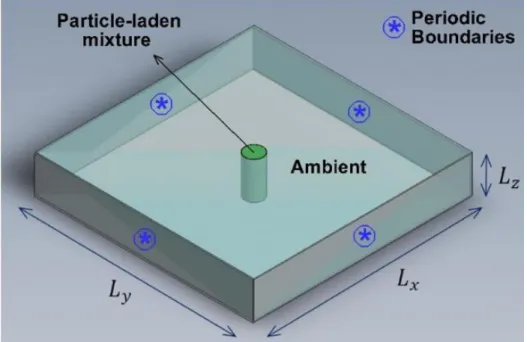
The simulations are carried out inside a rectangular computational domain (Figure 2-5) of dimensions 𝐿𝑥× 𝐿𝑦× 𝐿𝑧. Periodic boundary conditions are imposed
along the 𝑥 and 𝑦 directions. No-slip and free-slip conditions are imposed for the continuous phase along the bottom (𝑧 = 0) and top (𝑧 = 1) walls, respectively. Mixed and Neumann boundary conditions are imposed for the particle phase at the top and bottom walls, which translate into zero particle net flux and zero particle resuspension, respectively. {𝑎𝑡 𝑧 = 1 1 𝑆𝑐 𝑅𝑒 𝜕𝜙 𝜕𝑧 − 𝑉𝑠𝜙 = 0} ; {𝑎𝑡 𝑧 = 0 𝜕𝜙 𝜕𝑧 = 0} . (2-6)
2.3 Extended Box Model
Gravity currents resulting from planar and cylindrical fixed volume releases will remain planar, and axisymmetric as they spread out. On the other hand, most gravity
33
currents resulting from non-canonical configurations (non-planar and non-cylindrical) will spread in a manner that greatly depends on the initial shape of release. A simple, widely used, approach such as the box model provides a basic tool to quickly predict the front velocities of gravity currents resulting from canonical setups (planar and axisymmetric). The box model is a bold approximation (Figure 2-6) that assumes a planar (resp.
cylindrical) current to advance as a set of height-diminishing rectangles (resp. disks) of length 𝑥𝑓(𝑡) (resp. radius 𝑟𝑓(𝑡)) and height ℎ𝑓(𝑡). Each of these variables (length/radius
and height) is a unique function of time 𝑡. They are related by the Froude front condition as well as mass conservation. For a cylindrical current, the box model equations are
d𝑟𝑓 dt = 𝐹𝑟 ∙ √ℎ𝑓 (2-7) 1 2𝜋𝑟𝑓 2ℎ 𝑓 = 𝐼𝑛𝑖𝑡𝑖𝑎𝑙 𝑣𝑜𝑙𝑢𝑚𝑒 = 𝑐𝑜𝑛𝑠𝑡𝑎𝑛𝑡 (2-8)
where 𝐹𝑟 is the Froude function of order unity which depends on the height ratio between the current and the surrounding ambient. The above equations have been rendered non-dimensional using the same length and time scales introduced in the previous section on direct numerical simulations.
The box model is well suited for canonical problems resulting from planar and cylindrical releases, nonetheless, for non-canonical problems, it fails to capture the dependence on the initial shape. The reason for this failure is simple. The box model treats the current as one body as it homogenizes the flow properties (velocity and height) and neglects any spatial variations that might be present. For non-canonical releases, the velocity and height of the release must be allowed to vary along the interface.
34
The present section will provide details on the proposed extended box model (EBM). First, EBM constitutes a set of coupled algebraic and partial differential equations 𝑢𝑓 = 𝐹𝑟 ∙ √ℎ𝑓 (2-9) { 𝜕𝑥𝑓 𝜕𝑡 = 𝑢𝑓 𝜕𝑦𝑓/𝜕𝑠 √(𝜕𝑥𝑓/𝜕𝑠) 2 + (𝜕𝑦𝑓/𝜕𝑠) 2 𝜕𝑦𝑓 𝜕𝑡 = 𝑢𝑓 −𝜕𝑥𝑓/𝜕𝑠 √(𝜕𝑥𝑓/𝜕𝑠) 2 + (𝜕𝑦𝑓/𝜕𝑠)2 (2-10a) 𝜕𝜎 𝜕𝑡 = 𝑢𝑓 (2-10b) 𝜕𝜎ℎ𝑓 𝜕𝑡 = 0 (2-11)
The above set of equations describe the evolution of a gravity current front in the 𝑥-𝑦 plane. The independent variables 𝑠 and 𝑡 represent the distance measured along the circumference of the front and time, respectively. The subscript 𝑓 denotes front values, and {𝑥𝑓(𝑠, 𝑡), 𝑦𝑓(𝑠, 𝑡)} mark the location of the front in the 𝑥-𝑦 plane (Figure 2-7). The
height and outward normal velocity of the front correspond to ℎ𝑓(𝑠, 𝑡) and 𝑢𝑓(𝑠, 𝑡),
respectively. An additional variable, namely the area per arc length 𝜎(𝑠, 𝑡) is also used in the model. An integration of 𝜎(𝑠, 𝑡) over the entire arc length of the advancing front (perimeter of the current) will yield the total area covered by the platform of the
advancing current. All variables are rendered dimensionless using the same scales as in section 2.2. Equations (2-9), (2-10) and (2-11) refer to the Froude front condition, kinematic relations and mass conservation, respectively.
35
Analytical solutions of (2-9)-(2-11) are not feasible in the case of arbitrary initial patches, however, the system may be solved numerically. Its solution is far easier and faster than the direct numerical simulations discussed in section 2.2. Details about the numerical procedure used for solving (2-9)-(2-11) are hereby presented.
2.3.1 Initial Condition
The first step is providing the initial condition for the various variables. We start by defining the shape of the release. Let us consider for example the rounded
rectangular shape in Figure 2-2 and discretize the front using a set of equidistant points. The coordinates of these points represent the initial conditions for 𝑥𝑓 and 𝑦𝑓.
We consider full depth releases (where the initial height of the current inside the hollow cylinder is the same as that of the surrounding ambient), and therefore the initial non-dimensional height is set to unity at the discretized points.
The front velocity is straightforwardly calculated from the height using the Froude condition (2-9). We choose the empirical relation of Huppert-Simpson (1980) for the Froude number function
𝐹𝑟 = min (ℎ𝑓−1/3, 1.19). (2-12)
Finally, the initial condition for 𝜎 comes from the partitioning of the initial shape. The initial shape is partitioned geometrically by extending normal (to the front) lines inwards. These normal lines will initiate at the midpoint of each segment connecting 2
consecutive Lagrangian points (Figure 2-8). Because of the point symmetry of the rounded rectangle (RR) (the RR is symmetric w.r.t. the 𝑥 and 𝑦-axes), these (normal) lines will intersect the major and minor axes of the RR to form the sub volumes shown in Figure 2-8. Each sub volume has a corresponding segment along the front. The
36
centers of each of these segments coincide with the Lagrangian points {𝑥𝑓,𝑦𝑓}. The
initial value of 𝜎 may be easily calculated by dividing the surface of each sub volume by the corresponding front segment length
𝜎 = 𝐴𝑟𝑒𝑎
𝐿𝑒𝑛𝑔𝑡ℎ . (2-13)
The extended box model generalizes the classical box model (Huppert & Simpson 1980; Dade & Huppert 1995), in several ways. Despite these generalizations, the extended box model involves significant approximations. (H1) The volume of initial release is partitioned geometrically with inward propagating lines (perpendicular to the front) and accordingly different sub-volumes are assigned to the different portions of the front. (H2) As the current propagates, the height of the current is not taken to be a constant over the entire release. It varies along the front depending on the local speed of propagation. (H3) The velocity of propagation is taken to be normal to the front. Since there is variation in the height of the current along the front, it can be expected that there is some tangential flow (tangential velocity) induced by this variation in the current height. However, at the front, since the pressure gradient normal to the front is expected to far exceed the tangential gradient, the current velocity is expected to be
predominantly normal to the front. (H4) Finally we assume that even in the present case of non-axisymmetric propagation Huppert-Simpson front relation can be used to
express the front velocity in terms of local front height1. These assumptions are
examined with the help of direct numerical simulations in Chapter 5 section 5.
37 2.3.2 Time Integration and Spatial Discretization
Once the initial conditions are known, we march in time using a third order low-storage, explicit Runge-Kutta scheme and an eighth order central finite difference scheme for the spatial derivatives (with periodic boundary conditions). Each time step consists of two stages. The first is an intermediate stage where the governing equations (2-9)-(2-11) are integrated. At the end of this stage, because of the azimuthal variations, the Lagrangian points are no longer equidistant. Each sub-volume associated with a Lagrangian point is then assumed to be homogeneously distributed (along the front) between its two adjacent midpoints (think of volume per unit length along the front).
The second stage involves remapping the non-equidistant Lagrangian points to render them equidistant along the front. This step is necessary, especially in the case of concave corners, as in the plus-configuration for instance, as Lagrangian points may cross each other causing the front to fold on itself. This problem is classically
encountered in Lagrangian techniques such as Front Tracking approaches (Unverdi & Tryggvason 1992). Once the points are remapped, new midpoints are calculated and the sub-volumes of the release associated with each new Lagrangian point is
computed. Then a step of redistributing the sub-volumes per unit arc length (𝜎ℎ𝑓) is
performed, and this step preserves the total volume of the release. Finally 𝑢𝑓 and ℎ𝑓 are
interpolated at the new equi-spaced Lagrangian points.
Let us denote the intermediate stage by *. Then, if we start with a set of points {(𝑥𝑓)𝑖𝑛, (𝑦
𝑓)𝑖𝑛, (𝑢𝑓)𝑖𝑛, (ℎ𝑓)𝑖𝑛, (𝜎)𝑖𝑛}, (where superscript 𝑛 denotes a (known) quantity at the
present time, and subscript 𝑖 marks the 𝑖𝑡ℎ Lagrangian point), marching in time takes us
38 {(𝑥𝑓)𝑖𝑛, (𝑦 𝑓)𝑖𝑛, (𝑢𝑓)𝑖𝑛, (ℎ𝑓)𝑖𝑛, (𝜎)𝑖𝑛} (2-9)−(2-11) → {(𝑥𝑓)𝑖∗, (𝑦 𝑓)𝑖∗, (𝑢𝑓)𝑖∗, (ℎ𝑓)𝑖∗, (𝜎)𝑖∗} (2-14)
As previously mentioned, the Lagrangian points {(𝑥𝑓)∗, (𝑦𝑓)∗} will not necessarily be
equidistant along the arc length even when {(𝑥𝑓)𝑛, (𝑦𝑓)𝑛} are equidistant along the arc
length at time 𝑡𝑛. To render {(𝑥𝑓)∗, (𝑦𝑓)∗} equidistant, we first calculate the perimeter of
the front (at the intermediate * stage) by connecting the Lagrangian points with straight segments. From the ratio of the perimeter to the number of points, we compute the required separation distance at the new time step to be Δ𝑛+1
Δ𝑛+1= 𝑃𝑒𝑟𝑖𝑚𝑒𝑡𝑒𝑟∗
𝑁𝑢𝑚𝑏𝑒𝑟 𝑜𝑓 𝑝𝑜𝑖𝑛𝑡𝑠 . (2-15)
A point is then (randomly) fixed and each neighboring point is adjusted along the arc length to arrive at an equidistant set of points (with respect to the front at the
intermediate * stage) with spacing Δ𝑛+1.
Once the Lagrangian points are remapped to {(𝑥𝑓)𝑛+1, (𝑦𝑓)𝑛+1}, new midpoints
are calculated (by again remaining along the arc length of the intermediate stage). Each Lagrangian point now resides at the center of a segment bounded by the newly
calculated midpoints. As previously mentioned, each sub-volume (at the intermediate stage), is assumed to be homogeneously distributed (along the front) between its two adjacent midpoints. The task now is to associate a sub-volume to each of the remapped points {(𝑥𝑓)𝑛+1, (𝑦𝑓)𝑛+1}. This sub-volume is again bounded by the newly calculated
midpoints. This step can be thought of as having an arc composed of multiple segments of different lengths 𝑙𝑖 bounded by the midpoints of the Lagrangian points (Figure 2-9).
Each segment is associated to a sub-volume and has a certain (volume per unit length) value (Κ𝑖). The total volume of the current is recovered from the summation over all
39
segments ∑𝑁𝑖=1𝑙𝑖Κ𝑖 = 𝐼𝑛𝑖𝑡𝑖𝑎𝑙 𝑉𝑜𝑙𝑢𝑚𝑒, where 𝑁 is the total number of segments (or
number of Lagrangian points).
In a continuous (non-discretized) framework, the volume redistribution step may be described as follows. The volume of a differential element along the front (𝑑𝑉) is given by
𝑑𝑉 = 𝜎ℎ𝑓𝑑𝑠 . (2-16)
The total volume 𝑉 is recovered from a closed line integral along the front
𝑉 = ∮ 𝑑𝑉 = ∮ 𝜎ℎ𝑓𝑑𝑠 . (2-17)
At the intermediate stage, each (discretized) sub-volume is defined as Δ𝑉𝑖∗ = 𝜎
𝑖∗ℎ𝑓𝑖∗Δ𝑠𝑖∗ , (2-18)
where Δ𝑠𝑖∗ is the length of the segment centered around the Lagrangian point 𝑝𝑖∗ of
coordinates (𝑥𝑓𝑖∗, 𝑦𝑓𝑖∗). For the total of the 𝑁 segments centered around the 𝑁
Lagrangian points, the total volume is the summation 𝑉∗= ∑ 𝜎
𝑖∗ℎ𝑓𝑖∗Δ𝑠𝑖∗ 𝑁
𝑖=1
. (2-19)
After remapping of the Lagrangian points, the redistributed sub-volumes become Δ𝑉𝑖𝑛+1 = (𝜎ℎ
𝑓)𝑖𝑛+1Δ𝑠𝑖𝑛+1 , (2-20)
where the product (𝜎ℎ𝑓)𝑖𝑛+1 is obtained from the intermediate * stage as follows
(𝜎ℎ)𝑖𝑛+1 = ∑ 𝛼
𝑖𝑗𝜎𝑗∗ℎ𝑓𝑗∗ 𝑁
𝑗=1
(2-21) where the fraction 𝛼𝑖𝑗 is the ratio of the intersection of Δ𝑠𝑗∗ and Δ𝑠𝑗𝑛+1 divided by the
40 𝛼𝑖𝑗 =
Δ𝑠𝑗∗∩ Δ𝑠𝑗𝑛+1
Δ𝑠𝑗∗ . (2-22)
Let us consider the simple example shown in Figure 2-9. The boundaries of each segment (Figure 2-9A) can be thought of as the midpoints (thick dashes) of the Lagrangian points at the intermediate stage denoted by the asterisk (*). When the Lagrangian points are remapped in Figure 2-9B (to render them equidistant), the newly calculated midpoints will mark the new boundaries of the segments at the 𝑛 + 1 time step. Each segment (at the 𝑛 + 1 time step) might constitute of different portions of the (non-uniform) segments at the * stage. At the end of this step, the sub-volumes per unit arc length (𝜎ℎ𝑓) are obtained at the 𝑛 + 1 time step.
The height at the remapped points (ℎ𝑓𝑛+1) is then found by linear interpolation
from the intermediate * stage, and the velocity is calculated form the Froude condition. Finally, the area per arc length 𝜎𝑛+1 is the ratio of (𝜎ℎ
𝑓)𝑛+1 to the interpolated height
ℎ𝑓𝑛+1.
The extended box model (EBM) is a simple model that is primarily designed to capture the dependence of the flow (front location) on the initial shape of release. It will be shown in the subsequent chapters, that despite its simplicity, it can correctly capture the preferential spreading directions of non-axisymmetric gravity currents.
41
Figure 2-1. Isometric view of experimental setup. For the enlarged view at the bottom right, the tank and the motorized axes support have been hidden to allow for an unobstructed view of the laser.
Figure 2-2. Isometric view of the right-angled hollow cylinders. The dimensions of the cross-sections are in mm.
42 Figure 2-3. Measuring range of laser.
Figure 2-4. The large pixel intensity jump across the interface (close to an order of magnitude) allows the front to be easily identified.
43 Figure 2-5. Schematic of the numerical domain.
44
Figure 2-7. Schematic of extended box model. (𝑥𝑓(𝑠, 𝑡), 𝑦𝑓(𝑠, 𝑡)) denote the local
position, ℎ𝑓(𝑠, 𝑡) the height, 𝑢𝑓(𝑠, 𝑡) the outward normal velocity of the front
and 𝜎(𝑠, 𝑡) the area per arc length. The independent variables 𝑠 and 𝑡 denote the distance measured along the circumference of the front and time,
respectively.
Figure 2-8. Initial partitioning for the EBM for the rounded rectangle (left) and plus shape (right). The equidistant Lagrangian points are shown on the front as black circular disks. Each Lagrangian point is associated with a sub-volume. The sub-volumes are not necessarily equal.
45
Figure 2-9. Remapping of Lagrangian points and volume redistribution. 𝑝𝑖−1∗ 𝑝𝑖∗ 𝑝𝑖+1∗ 1 A 𝑝𝑖−1𝑛+1 𝑝𝑖𝑛+1 𝑝𝑖+1n+1 1 1 B
46 CHAPTER 3
LONG-LASTING EFFECT OF INITIAL CONFIGURATION IN GRAVITATIONAL SPREADING OF MATERIAL FRONTS
3.1 Background
Consider an accidental collapse or a skilled demolition of a building vertically on itself. The emerging debris cloud will quickly invade a wider region that greatly
surpasses the bounds of the demolished building. During the infamous 9/11 attack, the tidal wave of dust and debris enveloped much of the lower Manhattan. The gravitational spreading of these destructive debris clouds, as seen in Figure 3-1, sensitively depends on the building’s shape. The non-axisymmetric nature of the resulting lobe-like structure is persistent over a significant time and cannot be predicted by current models. This counter-intuitive behavior of initial condition-dependent spreading of material fronts is not unique to debris clouds, and is applicable to a variety of geophysical flows as demonstrated in this paper. Debris clouds belong to the family of gravity currents which are observed in various natural situations. The manner in which these flows spread has important implications for oil spills (Hoult 1972), accidental toxic gas releases (Britter 1989, Gröbelbauer 1993), fire propagation (Doyle & Carlson 2000), turbidity currents (Meiburg & Kneller 2010), pyroclastic flows (Faillettaz et al. 2004), avalanches
(Hopfinger 1983, Faillettaz et al. 2004) and storms (Hall et al.1976). These flows are driven by a difference in density either stemming from temperature, salinity or
suspended sediments.
This chapter has been previously published “Zgheib, N., Bonometti, T., & Balachandar, S. 2014.
Long-lasting effect of initial configuration in gravitational spreading of material fronts. Theoretical and