En vue de l'obtention du
DOCTORAT DE L'UNIVERSITÉ DE TOULOUSE
Délivré par :
Institut National Polytechnique de Toulouse (INP Toulouse) Discipline ou spécialité :
Dynamique des fluides
Présentée et soutenue par :
M. LUIS MIGUEL SEGUI TROTH le mardi 14 novembre 2017
Titre :
Unité de recherche : Ecole doctorale :
Multiphysics coupled simulations of gas turbines
Mécanique, Energétique, Génie civil, Procédés (MEGeP)
Centre Européen de Recherche et Formation Avancées en Calcul Scientifique (CERFACS) Directeur(s) de Thèse :
M. LAURENT GICQUEL
Rapporteurs :
M. EDWIN VAN DER WEIDE, UNIV. TWENTE ENSCHEDE PAYS-BAS M. GUILLAUME HOUZEAUX, BARCELONA SUPERCOMPUTING CENTER
Membre(s) du jury :
M. NICOLAS GOURDAIN, ISAE-SUPAERO, Président M. FRANCK NICOUD, UNIVERSITE DE MONTPELLIER, Membre
M. LAURENT GICQUEL, CERFACS, Membre Mme KARINE TRUFFIN, IFPEN, Membre
Acknowledgements
I would like to start thanking the members of the Jury for accepting to evaluate my work and for their time to review the manuscript. Their comments and punctualizations have helped to improve the quality of the manuscript and also provided paths to follow in the future.
I cannot neglect the importance of the Marie Curie Project COPA-GT that allowed me to come to CERFACS in the first place. The financial support from the European Union changed my life by granting me the chance of coming to France and joining such an incredible team.
More specifically, a special thank you goes to my supervisors Laurent and Florent for their support and help from the first day. We encountered a tough subject but after hard work from all parts, I want to think we have managed to put another stone towards the improvement of numerical schemes and to the understanding of turbine blade flows. Their contribution was not only limited to these topics but also to other soft skills and their insistence to believe in myself; something that I am still working on.
This thesis would not be the same without the contribution from Guillaume and Julien to the numerical part. Thank you for your time on a subject that did not concern you directly, for your patience and time for discussions that were so fruitful but also enjoyable.
Also, a great contributor to this thesis has been Jérôme. Many discussions concerning a large variety of themes have taken place during these years and have proven to be very useful. I don’t think I can mention all of them so I’ll just say that they were a lot.
Of course, I cannot forget the whole permanent CFD (and COOP) team of CERFACS, led so well by Thierry. I have had the opportunity to interact with the whole team (Benedicte, Olivier, Gab, Eléonore, Jérôme, Antony and Antoine) during or after the PhD. Also to the ’externals’ such as Franck and Stéphane who helped me both before and during the PhD.
To all the administration team, it has been great to share the corridors of the first floor with you that were always full of laughter which translated into a great atmosphere. Nothing would be the same without Chantal, Michèle, Dominique, Marie, Nicole, Brigitte, Lydia...
It is indispensable to mention all the CSG team who are always helpful in the moments of greatest need (something that happens quite often). Their patience and knowledge is without doubt one of the most important assets of the whole group.
I had the opportunity to coincide with many PhD students and PostDocs with which I had not only the luck to work with but also to spend time outside our offices. Both to the ones who were already here when I arrived (Dimitris, Ignacio, Corentin, Lucas, Laure, Manqi...) and to those who I met after (Pierre, Omar, Dario, Luc, Franchine, Félix, Lulu, Nico, Mélissa, Majd, Romain, Pamphile...). A special mention goes to Francis and Thomas whom I had the luck to share the office with. To all members of the EAC: I’m sure this next season will be better than the last, we just need to keep recruiting!
To all my friends from Tenerife, Seville and Toulouse who have understood the difficulty behind what I was confronting and weren’t too hard on me when I turned down a beer because I had to work. We will have more time now.
Finally, I want to thank my family for their support during so many years. To my parents for their patience and continuous support even in the distance and on days when my temper wasn’t the best. To my brother, I’m sorry to have been so hard during our math lessons when we were younger. I really am trying to improve this last part now that Olivia is here.
want to enjoy what comes next beside you and Olivia. Let’s get down to business.
La inspiración existe, pero tiene que encontrarte trabajando. Pablo Picasso
Contents
1 General introduction 1
1.1 CFD, how did we get here? . . . 1
1.2 Industrial interest for CFD . . . 4
1.3 Gas Turbines . . . 6
1.4 Objectives . . . 8
I Modelling and Numerics
11
2 Introduction to Modelling and Numerics 15 2.1 Free-stream turbulence based modelling . . . 162.2 Near-wall turbulence modelling . . . 20
2.3 Meshes for LES . . . 22
2.4 Spatial Discretization . . . 23
2.4.1 Finite Differences (FD) . . . 26
2.4.2 Finite Elements (FE) . . . 27
2.4.3 Finite Volumes (FV) . . . 27
2.4.4 Residual distribution schemes (RD) . . . 28
2.5 Temporal integration . . . 29
3 Numerics of AVBP 33 3.1 The cell-vertex approach . . . 34
3.1.1 Cells and metric definition . . . 35
3.1.2 Residual calculation . . . 36
3.2 Convection schemes in AVBP . . . 37
3.2.1 Lax-Wendroff scheme . . . 37
3.2.2 TTG numerical schemes . . . 39
3.3 Diffusion schemes in AVBP . . . 46
3.3.1 FV 4 operator . . . 47
3.3.2 FE 2 operator . . . 48
3.4 Numerical scheme stability constraints . . . 49
3.4.1 CFL number . . . 49
3.4.2 Fourier number . . . 49
3.5 Artificial viscosity (AV) . . . 50
3.5.1 The operators . . . 50
3.5.2.1 The Jameson sensor . . . 51
3.5.2.2 The Colin sensor . . . 51
3.6 Boundary conditions (BC) . . . 52
4 Spectral properties of the AVBP schemes 55 4.1 Concepts and definitions . . . 58
4.2 Consistency results . . . 59
4.3 von Neumann stability analysis . . . 60
4.3.1 1D analysis . . . 62
4.3.2 2D analysis . . . 68
II Application to a complex geometry: LS89
77
5 Introduction to LS89 simulations 81 5.1 Application and validation of LES for a complex turbomachinery flow . . . 815.1.1 Boundary layer transition . . . 84
5.2 LS89: Experiments and literature review . . . 88
5.3 LS89: Operating points . . . 91
5.4 Mesh resolution . . . 93
5.5 Numerics and modelling . . . 95
5.5.1 Turbulence injection . . . 96
5.6 Characteristic flow time, convergence and simulation cost . . . 97
6 LES predictions of MUR129 and MUR235 99 6.1 MUR129 predictions . . . 99
6.2 MUR235 predictions . . . 102
6.2.1 M1 mesh predictions using synthetic turbulence injection . . . 103
6.2.2 Grid resolution impact . . . 118
6.2.3 Preliminar conclusions from the parametric study . . . 123
6.3 Temporal evolution of near-wall turbulence . . . 124
6.4 Conclusions . . . 138
7 LS89 Numerical Aspects and associated analyses 139 7.1 Advanced stability analysis of AVBP . . . 143
7.1.1 Amplification matrix . . . 144
7.1.2 1D cavity eigenmode . . . 148
7.1.3 Application to a Poiseuille flow . . . 151
7.2 Development of a new numerical closure . . . 153
7.2.1 1D profile between walls . . . 154
7.3 Node and dual cell centroid conundrum . . . 157
7.3.1 1D convection of an acoustic wave . . . 158
7.3.2 Perspectives . . . 162
7.4 Conclusions . . . 162 General Conclusions and Perspectives 165
CONTENTS
Appendices 169
A General equations 171
A.1 LES governing equations . . . 173
B Sub-grid scale models 177 B.1 Sub-grid models available in AVBP . . . 178
B.2 Smagorinsky model . . . 178
B.3 WALE model . . . 178
B.4 Sigma model . . . 179
C Precursor methodology 181 C.1 Methodology for precursor simulation . . . 182
C.2 Test case: Turbulent channel . . . 185
D Convergence aspects 191 E Development of one iteration calculation 195 E.1 First order temporal derivative for triangular elements, L term . . . 195
E.2 First order temporal derivative for quadrilateral elements, L term . . . 197
E.3 Second order temporal derivative for quadrilateral elements, LL term . . . 199 F Resampling Strategies to Improve Surrogate Model-based Uncertainty
Quan-tification - Application to LES of LS89 201
List of Figures
1.1 IBM computer in 1955, capable of performing 3750 operations per second. Total
memory of approximately 10 kbytes. . . 4
1.2 Evolution of equations solved for similar problems throughout the years [83]. . . 5
2.1 Spectrum of an homogeneous isotropic turbulent flow [194]. . . 17
2.2 Mesh comparison between structured and unstructured meshes. . . 23
2.3 Discretization approaches [45], a) cell-vertex, b) cell-centre and c) vertex-based approach. . . 25
2.4 Partitioning of cells in AVBP [29] duplicates the number of nodes affected by the partition. Definition of primary and dual cells around a target node are also shown. . . 26
3.1 Residuals at primary (white) and dual (shaded) cells. . . 34
3.2 Definition of cell-vertex metric. . . 36
3.3 Detail of mesh dual cell. . . 45
3.4 Complete connectivity around node j for FV 4 . Gradients are required in all the primary cells and the divergence operator is applied only to the shaded cell. 47 3.5 Complete connectivity around node j for FE 2 . Gradients are required in all the primary cells and the divergence operator is applied only to the shaded cell. 48 4.1 Group velocity as shown by Vichnevetsky and Bowles [187]. Three snapshots of a spatially evolving signal highlights the dispersion it undergoes. . . 56
4.2 Chequerboard mode and washboard modes on left and right respectively. . . 57
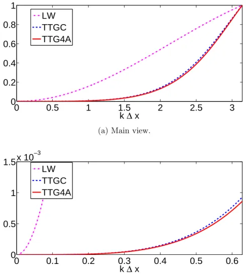
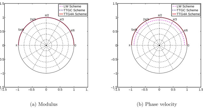
4.3 Amplification factor of various schemes for CFL=0.1. . . 63
4.4 Dissipation error using the amplification factor of various schemes for CFL=0.1. 64 4.5 Dispersion error using the amplification factor of various schemes for CFL=0.1. . 65
4.6 Amplification factor of various schemes for CFL=0.3. . . 66
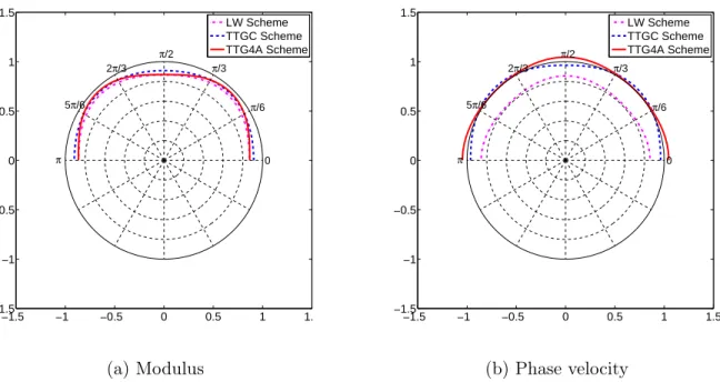
4.7 Amplification factor of various schemes for CFL=0.5. . . 67
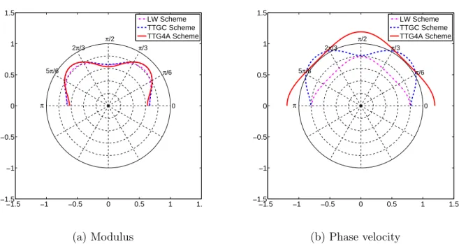
4.8 Amplification factor of various schemes for CFL=0.7. . . 67
4.9 Amplification factor of various schemes for CFL=0.3 at 8h wavelengths. . . 70
4.10 Amplification factor of various schemes for CFL=0.7 at 8h wavelengths. . . 70
4.11 Dissipation errors 8h wavelengths. . . 71
4.12 Amplification factor of various schemes for CFL=0.3 at 4h wavelengths. . . 71
4.13 Amplification factor of various schemes for CFL=0.7 at 4h wavelengths. . . 72
4.14 Dissipation errors 4h wavelengths. . . 72
4.15 Dispersion errors 4h wavelengths. . . 72
4.17 Amplification factor of various schemes for CFL=0.7 at 3h wavelengths. . . 73
4.18 Amplification factor of various schemes for CFL=0.3 at 2h wavelengths. . . 74
4.19 Amplification factor of various schemes for CFL=0.7 at 2h wavelengths. . . 75
5.1 Boundary layer distribution in terms of Reynolds number [140]. . . 83
5.2 Formation and evolution of turbulent spots [120]. . . 84
5.3 Instability process in natural transition as described in [89]. . . 85
5.4 Sources of streak generation in boundary layers [120]. . . 86
5.5 Separation mechanism instabilities [120]. . . 87
5.6 Isentropic Light Piston Compression Tube facility at VKI facilities. . . 89
5.7 Geometrical detail of the LS89 blade. . . 90
5.8 Computational domain used for the simulation of the LS89 configuration. . . 92
5.9 Measured turbulence intensity dependency on the grid position. Positions A-D correspond to different grid locations. . . 93
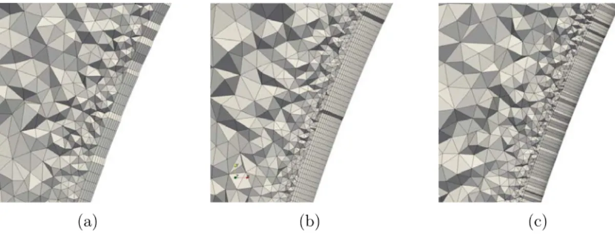
5.10 LLS89 mesh at inlet for (a) M1 mesh (b) M2 mesh (c) M3 mesh. . . 94
5.11 LS89 mesh in near-wall region as highlighted by the box represented on Fig. 5.10a (a) M1 mesh (b) M2 mesh (c) M3 mesh. . . 94
5.12 LS89 mesh at trailing edge for (a) M1 mesh (b) M2 mesh (c) M3 mesh. . . 95
5.13 Global process of the precursor technique; fluctuations extracted from the pre-cursor domain are transferred to the inlet of the main domain. . . 96
6.1 MUR129 operating point for M1 mesh. a) Q-criterion coloured by vorticity. Background plane represents the|r⇢| ⇢ b) y+distribution along curvilinear abscissa for M1. . . 100
6.2 Spectral composition of the pressure signal at probes A and B. . . 101
6.3 Heat transfer coefficient of MUR129. . . 102
6.4 Shear stress field on blade surface. Background plane represents the |r⇢| ⇢ . . . 103
6.5 MUR235 operating point. a) Q-criterion coloured by vorticity. Background plane represents the |r⇢| ⇢ b) Stretched vortices around leading edge of the blade represented by Q-criterion coloured by spanwise velocity. . . 104
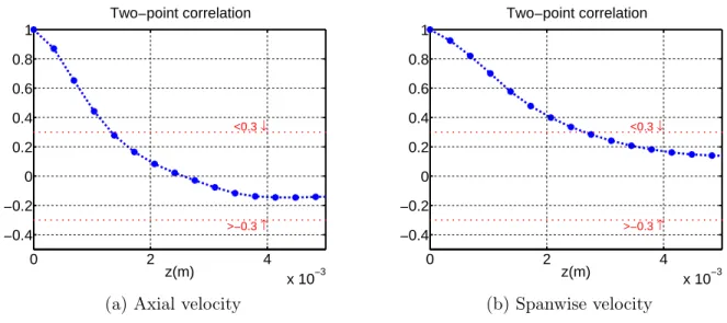
6.6 Axial and spanwise velocity correlations in spanwise direction. . . 105
6.7 Heat flux comparison of MUR129 and MUR235 operating points using syn-thetic injection methods when required. . . 105
6.8 Turbulent intensity decay at inlet channel upstream from blade. . . 107
6.9 Isentropic Mach number comparison of turbulence injection methods for MUR235 operating point for M1 grid. . . 108
6.10 Shear stress comparison of turbulence injection methods for MUR235 operating point for M1 grid. . . 108
6.11 Heat flux comparison of turbulence injection methods for MUR235 operating point for M1 grid. . . 109
6.12 Coherent structures representation for a) 6% b) 18% turbulent intensity at the inlet using M1. . . 110
6.13 Interaction between free-stream vortices and wall structures. . . 111
6.14 Displacement and momentum thickness along the suction side of the blade for M1 mesh. . . 112
LIST OF FIGURES
6.15 Shape factor on suction side at different abscissas in the transitioning region. . . 112
6.16 Tangential velocity profiles on suction side at different s/c. . . 114
6.17 Turbulent Kinetic Energy profiles along different stations on the suction side a) s/c = 0.3 b) s/c = 0.7 c) s/c = 1.1. . . 115
6.18 Instantaneous temperature field a) MUR129, b) MUR235 u=6%, c) MUR235 u=18%. . . 116
6.19 Modified geometry with three times initial spanwise domain. . . 117
6.20 Heat transfer coefficient comparison for different length scales. . . 118
6.21 Density gradient comparison for 18% turbulent intensity at inlet. . . 119
6.22 Spectral content of the pressure signal at probes A and B. . . 120
6.23 Trailing edge vorticity comparison between different meshes. . . 120
6.24 Heat flux comparison of MUR235 with fine mesh. . . 121
6.25 Isentropic Mach number comparison of MUR235 with three meshes and 6% turbulent intensity at inlet. . . 121
6.26 Shear stress comparison of MUR235 with three meshes and 6% turbulent in-tensity at inlet. . . 122
6.27 Heat flux comparison of MUR235 with three meshes and 6% turbulent intensity at inlet. . . 123
6.28 Turbulent viscosity comparison between a) M1 and b) M3 grids. . . 124
6.29 Shear stress field shown on the blade surface where each sphere corresponds to locations where probes were located. The region highlighted on the blade surface shows turbulent structures represented to the right of the figure. . . 126
6.30 Coloured field shows cross-stream (n-z) instantaneous distribution of streamwise velocity fluctuations at s/c = 0.8 . Arrows show normal (n) and spanwise (z) velocity vectors. . . 126
6.31 Coloured field shows streamwise (s-z) instantaneous distribution of streamwise velocity fluctuations at s/c = 0.8 at a) y+ = 5 b) y+ = 20. Arrows show normal and spanwise velocity vectors. . . 127
6.32 Temporal evolution of streamwise, normal and spanwise velocities at s/c = 0.7 and y+ = 10. . . 128
6.33 Temporal evolution of velocity fluctuations. Boxes show where the sensor is active and records the signal to be used. . . 128
6.34 Skewness of streamwise velocity fluctuations at various positions normal to the surface. . . 129
6.35 Quadrant analysis of boundary layer interactions [134]. . . 130
6.36 Velocity fluctuations at Position 4 of the a) M3 and b) M1 meshes. . . 131
6.37 Evolution at s/c = 0.5 of normal against streamwise fluctuation map for a) M3 b) M1 mesh. . . 131
6.38 Streamwise agains normal velocity fluctuations at various positions normal to the blade at s/c = 0.6 using M3 grid. . . 132
6.39 Streamwise agains normal velocity fluctuations at various positions normal to the blade at s/c = 0.8 using M3 grid. . . 133
6.40 Reynolds stresses separated in quadrants plotted as a function to the wall dis-tance. The streamwise position on the suction side corresponds to a) s/c = 0.4 b) s/c = 0.5 c) s/c = 0.6 d) s/c = 0.7 e) s/c = 0.8 f) s/c = 0.9. . . 135
6.41 Turbulence triangles at various locations normal to the blade and different
curvi-linear abscissa positions for M3 mesh. . . 137
7.1 Pressure field in wall region at an arbitrary position on the suction side of the blade for a) LW scheme b) TTG scheme c) crinkled slice of pressure field for LW. 140 7.2 Instantaneous surface pressure field on the suction side of the blade downstream the shock for a) TTGC scheme b) TTG4A scheme. . . 141
7.3 Border cell indicating primary and dual cells (discontinuous line). . . 143
7.4 Oscillations originated by round-off error example [79]. . . 144
7.5 Eigenvalues spectra obtained using the amplification matrix, [99]. . . 148
7.6 Initialization of the wave for the 1D cavity. . . 148
7.7 Eigenvalue distribution of LW USOT amplification matrix applied to a 1D cavity eigenmode. . . 149
7.8 Eigenvalue distribution of TTGC USOT amplification matrix applied to a 1D cavity eigenmode. . . 150
7.9 Eigenvalue distribution of LW CSOT amplification matrix applied to a 1D cavity eigenmode. The red circle highlights an eigenvalue located outside the unit circle which indicates an unstable mode. . . 150
7.10 Mesh used for amplification matrix test. . . 151
7.11 Eigenvalue distribution of USOT amplification matrix applied to a Poiseuille flow.152 7.12 Eigenvalue distribution of CSOT amplification matrix applied to a Poiseuille flow.153 7.13 Mesh used to impose the 1D acoustic profile sufficient to neglect possible border effects. . . 155
7.14 1D acoustic profile of the initial solution. . . 155
7.15 Dual cell of a border schemes indicating the centroid of primary cells with red crosses and the CMDC by the blue plus sign. . . 158
7.16 Excess noise. . . 159
7.17 Meshes used for the convection of an acoustic wave in a) Isotropic triangles b) Modified triangles c) Hybrid triangle-quad mesh. . . 159
7.18 Representation of a dual cell around node inside box highlighted in a) Fig. 7.17b b) Fig. 7.17c. Red crosses represent the centroid of each intersection of dual cell and primary cell. Deviation of CMDC to node is represented by the blue plus sign. . . 160
7.19 Pressure fluctuation profile in y direction at x = 0.5 where symbols and their corresponding meshes are: (4) Fig. 7.17a; ( ) Fig. 7.17b ; (⇥) Fig. 7.17c. . . 161
7.20 Test performed on alternative mesh where mesh is not stretched in the convection direction. . . 161
C.1 Spatial evolution of Taylor microscale in experimental study [16]. Marker curves represent various experimental results at different turbulence intensity levels. . . 184
C.2 Skewness of spatial velocity derivative measured experimentally [178]. . . 184
C.3 Channel geometry and boundary conditions. . . 185
C.4 Channel test case. a) Q-criterion coloured by vorticity b) Vorticity field on a x-y plane. . . 186
C.5 Spatial TKE decay comparison. a) TKE decay along axial direction b) View of the 10% inlet channel region. . . 187
LIST OF FIGURES
C.6 Spatial evolution comparison of Taylor microscale with numerical simulation. . . 187
C.7 Skewness of velocity gradient components in channel. . . 188
C.8 Spectrum comparison at inlet plane. . . 188
C.9 Ruu at inlet. . . 189
C.10 Ruu at outlet . . . 189
D.1 Heat transfer coefficient profile in most unsteady case for 18% turbulence using M1 mesh. . . 192
D.2 Heat flux histogram at a) s/c = 0.4 b) s/c = 0.6 c) s/c = 0.8. . . 193
E.1 Notation and definitions used for elements in AVBP. . . 196
E.2 Detail of mesh dual cell. . . 197
E.3 Dual cell mesh. x represent the centroid of the intersection Ke\ Cj and + is the global centroid of the cell. . . 197
List of Tables
3.1 Coefficients for the Two-Step Taylor Galerkin schemes implemented in AVBP. . 41
5.1 Geometrical parameters characterizing LS89 geometry. . . 89
5.2 Operation point conditions. . . 91
5.3 Mesh parameters for three meshes simulated. . . 95
5.4 Machine architecture description. . . 97
5.5 CPU detailed for various simulations. . . 98
6.1 Global performance for each value of turbulent intensity and spectrum injected. 107 6.2 Position of local probes in normal to blade direction. . . 129
7.1 Wave strength values obtained by Porta [143]. . . 156
7.2 TSOT closure terms using different time steps for the same order approximation. 156 7.3 TSOT closure terms using a constant time step for different order approximation.157 C.1 Variables imposed in each precursor simulation. . . 185
Nomenclature
Filter width
x Cell length in x direction, m
Wavelength, m
t Thermal diffusivity, W/(m.K)
R⌦j Cell-based residual
U Conservative variables vector ⌫ Kinematic viscosity, m2/s
⌫⌧ Turbulent viscosity, m2/s i Shape functions
⇢ Density, kg/m3
⌧w Wall shear stress, Pa
~ FC Convective fluxes ~ FV Viscous fluxes Dk ⌦j Distribution Matrix f Frequency, Hz H Total enthalpy
K Von Karman constant L Length, m
Mis Isentropic Mach number
p Pressure, Pa Pt Total pressure, Pa
Re Reynolds number T Temperature, K t Time, sec
Tt Total temperature, K
T KE Turbulent kinetic energy, J T u Turbulence Intensity V⌦j Cell volume
x+ Non-dimensional streamwise distance
y+ Non-dimensional wall-normal distance
z+ Non-dimensional spanwise distance
(U)RANS (Unsteady) Reynolds Averaged Navier-Stokes CFD Computational Fluid Dynamics
CFL Courant-Friedrichs-Lewy number DNS Direct Numerical Simulations FFT Fast Fourier Transform GT Gas Turbines
HPT High-Pressure Turbine LES Large Eddy Simulation
NSCBC Navier-Stokes Characteristic Boundary Conditions PSD Power Spectral Density
R Radius, m
RMS Root Mean Square SGS Sub-Grid Scale
Chapter 1
General introduction
Contents
1.1 CFD, how did we get here? . . . 1 1.2 Industrial interest for CFD . . . 4 1.3 Gas Turbines . . . 6 1.4 Objectives . . . 8
1.1 CFD, how did we get here?
To understand the development of humanity up to its present state, it would be difficult to contextualize the world as in 2017 without talking about Fluid Mechanics. Transport in ancient and current societies, energy transformation for common use or even developments in biomed-ical research would not be possible without fluids. Fundamental of Fluid Mechanics started with the hydrostatic theory, a contribution that is known to the non-specialized public such as Archimedes’ principle. The principle implies an incompressible fluid, an acceptable hypothesis for liquids, and allowed to develop architectural elements such as aqueducts or cisterns but also to explain the buoyant forces that keep a boat afloat. Likewise, to understand the atmosphere that surrounds the planet, it is necessary to balance the different forces applied to the air and the different pressures encountered in each layer. This is now known thanks to the contribu-tion of Pascal who introduced the concept of hydrostatic pressure. This same principle can be extended to many other fields such as biomechanics where equilibrium processes take place in the body of any human being. In short, many engineering applications rely on the most basic principles of fluids without even introducing the applications of fluid dynamics.
Of course, one might be tempted to think that considering the large space of time since the first developments done over more than 2000 years, the basics are today well understood. The problem of fluids is that even with all the powerful tools available today, predicting how a flow will establish still remains the greatest unresolved problem of classical physics. The ideal would be to find a general model capable of predicting the behaviour of any type of flow and solve it for each particular case. The first step in itself, although achieved in the context of Newtonian fluids, was not at all trivial and it took many centuries to be able to define the problem to
be solved. The validity of this model, represented by a set of equations, is currently one of the Seven Problems of the Millennium of the Clay Institute that questions the existence of the solutions and their unicity. However and despite the lack of such validation or demonstration, these equations are currently being heavily used and are the starting point of anybody willing to study flows in a Computational Fluid Dynamics (CFD) context.
Historically, the governing equations at hand are the today well-known set of Navier-Stokes equations, named after both Claude Navier and George Stokes. Their individual contributions were to introduce respectively, the viscous transport equations for an incompressible fluid and its extension to compressible fluids [14] responsible for the shear stress or heat transfer effects. Not mentioned explicitly, the reader may note that there is a loop in the process as only the viscous part of the equations is mentioned and so, an inviscid part must also exist. Due to the great number of publications and theorems already assigned to his name, Leonhard Euler is mentioned only for the inviscid part of the equations.
Many applications of these equations were found during the 19th Century and solutions to specific problems of interest were developed. To mention some, the solution to a laminar channel done by Poiseuille, or Reynolds, who determined that different flows could be classified depending on the ratio of inertial forces to viscous forces. Additionally, Reynolds introduced the idea of separating a mean component and a fluctuating component for a turbulent flow, leading to a Reynolds-average way of dealing with turbulence. The resolution of such complex problems required a reasonable hypothesis in each case, and thus, a limited applicability of the solution. From a physical point of view, it was important for the understanding of certain principles that although still not well mastered, set a ground for the study of many engineering applications such as turbomachines. From a mathematical point of view however, developments did not advance as fast as in the coming 20th century. One of the reasons for these mathemat-ical difficulties can be found in the nature of the equations.
The equations are written in terms of partial derivatives and some of the shortcomings of the methodologies developed until the 20th century were in part due to the lack of tech-niques to solve Partial Differential Equations (PDE). These relate to the the inability to find a mathematical functional space for an adequate solution to the problem. Indeed, although in-finitesimal calculus had been developed by notable mathematicians such as Newton or Leibniz, applications to this field were not found until many centuries later. The realization that the continuous equations could not be solved resurfaced the possibility to study them in a discrete way through numerical schemes or algebraic relationships. In that respect, contributions by Banach and Sobolev to functional analysis [27] and their future application to Finite Elements, were fundamental to a larger variety of spatial discretization techniques.
In terms of developments and associated interest from industry, one can easily identify the presence of an inflection point in the resolution of the system of equations’ history; before and after World War II. There is a general consensus that the first work in the context of what today is known as CFD was published by Richardson [149] and consisted in solving the Laplace equa-tion using a relaxaequa-tion technique. Another important achievement before this period was done by Lewy et al. [108] who defined one of the stability requirements for the resolution schemes.
1.1 CFD, how did we get here? The definition of the CFL number, known to any CFD practitioner, is due to this paper. Other contributions were done by Lax [103] who stated the theorem that produces the sufficient con-ditions of consistency and stability to guarantee the convergence of the discretization. The stability of the different methods was then continued by von Neumann and Richtmeyer in [188] who developed a methodology capable of determining the stability of the scheme under certain hypotheses.
Nowadays, past World War II progress still remains the panorama as no numerical scheme has yet managed to impose itself over others. And it is still in continuous development as the problems to be solved become more and more complex. Classical methods for spatial dis-cretizations such as Finite Differences, Finite Elements or Finite Volumes coupled with a time integration scheme are nowadays used regularly, as well as other methods such as the multi-grid approach. More recent methods such as Spectral schemes [195] or Lattice-Boltzmann [77] are increasing their presence in publications. The current tendency is to increase the order of the scheme, meaning that a higher accuracy is attained for the same number of degrees of freedom, compensated of course by a larger number of operations. However, there is a limit to these developments which introduces significant difficulties. This was found thanks to Godunov [70] who published in his thesis the theorem that carries his name. He stated that a scheme of order equal or higher than two is non-monotonic. This affirmation is a strong one as it requires for practically all type of schemes to introduce flux limiters or to suffer the consequences, namely the node-to-node oscillations, a deadbeat and purely numerical artifact.
While computers might seem the sine qua non of CFD as explicitly noted in its name, initial computations such as the ones done by Richardson [149] were not performed by a machine. It was after the war that developments in the military industry led to more powerful tools for the resolution of repetitive tasks. The classical Turing machines started to literally fill laboratories and Universities, see Fig. 1.1. Some of the most convinced precursors of machine-resolved task resolution were some of the great names in CFD, von Neumann and Lax. The arrival of ma-chines capable of solving costly operations for humans increased the interest in this discipline. This induced the growth in the number of publications focusing on numerical simulations, but also the number of groups developing new mathematical methods and applying them to prob-lems of industrial interest. The main initial issue from a coding point of view at the time was the difficulty of implementing the desired code and worst of all, the portability of this code for future machines. This issue might once again be of relevance as in recent years, the existence of GPU architectures or even quantum machines have shown their power and possible advantages. The exploitation of these machines seems to be the future and requires to adapt most codes to these new systems.
In any case, the future of scientific computing seems guaranteed and so, the continuous development of tools and results that may one day be of use.
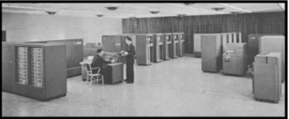
Figure 1.1: IBM computer in 1955, capable of performing 3750 operations per second. Total memory of approximately 10 kbytes.
1.2 Industrial interest for CFD
The rate of development of CFD has been greatly impacted by industrial needs. Developments in CFD required an investment that industry could provide while industry required means to reduce their costs using improved or complimentary methods to the traditional experimental procedures. This process is still taking place today because many tasks may not be put in place using industrial configurations, or at least not as regularly as required at an assumable cost. Industrial applications represent a challenge both in terms of geometry and flow physics. Geometrical difficulties arise as a result of the global optimization process leading to curved shapes which are difficult to represent. Flow physics are also a problem as highly turbulent flows are encountered in most of these industrial configurations. Higher levels of turbulence require more computational power and it was clear from the beginning to the precursors of CFD that computational power available at the time would inevitably limit the industrial applications. To circumvent this limit, the development of turbulence models appeared and contributions from Spalding [174] with the k-✏ model allowed to address turbulent flows. The model used at the time is still widely applied today and many variants have been developed since its first appearance [122].
In term of process and effective use of CFD by industry, one has to realize that in the aero-nautical industry, the first complete aircraft simulations were performed using potential flow theory in the 60-70s. Euler equations were then successfully applied in the following decade to a whole aircraft configuration. The optimization process did not start until the decade 90-00 using Euler equations, the Navier-Stokes equations being applied in the past decade [88] for the whole aircraft, see Fig. 1.2. Note that qualifying the simulation of a complete aircraft does not mean taking into account all of its components. In fact, most of the time the use of CFD is more or less frequent depending on the difficulty to capture the physics around the targeted domain and its relevance to the overall design process. For example, the ventilation system is important for the cooling of components and optimal comfort of passengers but of great difficulty to model due to all the possible sub-components of an aircraft present in a large configuration. This being
1.2 Industrial interest for CFD
Figure 1.2: Evolution of equations solved for similar problems throughout the years [83]. the case, use of CFD for this specific problem has been largely neglected until recently. Fuselage design or performance envelopes on the other hand have always been targeted since the gain in optimization is much more important. Today, it is possible to model complete aircrafts or cars but difficulties are still present when simulating vortex dominated transitional flows. This is the case for internal engine aerodynamics. Unsteady effects however govern most processes in a flow and turbulence models are in most cases insufficient for the correct prediction of the associated physics. It seems however clear to most of the community that the correct rep-resentation of these unsteady effects is critical to the manufacturers to produce better products. To this end, it is necessary to have a solver as well as the means to perform these simulations and the expertise required to analyze the results. Generally, CFD codes are not developed by the industry that uses them. If the problem is a multiphysics problem, it could be necessary to acquire multiple codes. In fact, each CFD code depending on its numerical approach inherently limits the range of problems it will be optimal for. The existence of dedicated codes for each discipline is hence common.
The appearance of the first CFD general-purpose code was PHOENICS, contemporary to one of the best-known commercial software that appeared a few years later and named FLU-ENT. Although the existence of solvers alone does not guarantee a sufficient basis for adequate CFD simulations, pre-processing and post-processing softwares are also required to create the necessary meshes and to be able to analyze the results. Large editors such as ANSYS provide the whole chain so it is a good option for many good manufacturers. The existence of such an offer could seem discouraging for smaller research groups to find their place in the industry market. However, future trends are always pursued by research groups, public or private, and remains their strength. It has been said that unsteady effects contribute largely to flows and Large Eddy Simulation (LES) is an alternative turbulence modeling approach to Reynolds-Averaged Navier Stokes (RANS), one that is feasible for industry in the coming years. The
gain behind this new approach is that modeling is reduced and more degrees of freedom are used, the fluid being treated as a fully dynamic and unsteady system. This different formalism usually requires different schemes and so, a completely different code. Additionally, LES re-quires an expertise that can be found in research groups and not so often in industry as the use of this methodology is still not common. Even with larger computers, a great effort must still be done to increase the efficiency and the applicability range for industry, namely through code parallelism. The access to this type of supercomputers is also an issue and although research groups are granted access to a large volume of CPU hours provided by national governments for research means, industrial partners must pay these accesses. This gives an edge to research departments to gain expertise that is then published and applied in future configurations com-ing from industry.
The industrial configurations of interest are here limited to gas turbines for the following. The interest of this thesis focuses on the possible means to obtain the solutions to the Navier-Stokes equations within the context of gas turbines. The study of gas turbines is bounded by the formalism chosen and corresponds to Large Eddy Simulations (LES) for the present document. There are two main questions to be answered in relation to the output provided by any CFD code when performing a gas turbine component simulation. First of all, is the code capable of producing an acceptable prediction of the flow at hand? Many codes presume they possess the required properties to be a usable code in industry. Some of these properties are that it is optimally parallelized, that it is portable on a large range of machines or that it contains the latest and most robust numerical methods. This last point is interesting as a per-fect comparison between codes and their numerical schemes is never possible, or complicated at the very least, for complex configurations. If however it is assumed that a fair compari-son can be done, it is reacompari-sonable to ask how well each code behaves when confronted to the complex cases they must solve and for which they were designed and financed. The second question relates precisely to the numerical methods behind each simulation: which is the best choice? For this document, the comparison between numerical methods is limited to only one code. Nevertheless, various numerical methods implemented in this same code are compared in simple and in complex configurations. These methods will be notably low-order versus high-order schemes (see Chap. 3) and comparisons to literature results are performed when available.
1.3 Gas Turbines
Gas Turbines (GT) have been used to power aircraft since the 1930s when thrust generating aeroengines were first used. Due to their higher power-to-weight ratio these engines are exten-sively used either to power aircraft or produce electrical energy in an effective and adaptive way. Aircraft engines are subject to a large range of operating conditions on a daily basis where it must perform safely. From take-off to cruise, from the Andes to the Sahara desert the variability of the atmosphere must not interfere with the performance limits of the aircraft and thereby its engines. This large envelope of operating points introduces difficulties in many aspects including combustion requirements. It is necessary to operate and maintain an efficient but at the same time quiet and ’green’ combustion.
1.3 Gas Turbines Historically, there has been little need for clean combustion requirements, so liability and efficiency have been the main targets of existing aircraft engine designs. Reliability was an eas-ily measured parameter which has mainly been addressed by performing multiple tests for the different modules of the engine. The exercise hence, resumed to finding the best compromise to operate the engine for as long as possible. When dealing with efficiency, it began to be a prob-lem once the aircraft industry started to grow exponentially and fuel reservoirs were no longer considered as infinite. Industry became more competitive and companies began to find out that preservation of their market shares started to be a difficult exercise which forced them to be in continuous evolution, a context where research becomes crucial. At the same time, external agents such as governments or regulation agencies started adding more constraints to the whole process of design and operation. A direct consequence of such a stringent industrial context is that it is no longer possible to produce and test all the thought innovations that might occur within an engineering process. Experience can provide an approximative assessment of a given design but such an intuitive decision making carries either a lot of risks or conversely prevent disruptive and potentially highly efficient solutions. Decision taking is definitely not eased by the flow encountered in such systems which results from the different aspects of the physics in the engine which are highly coupled. Despite this fact, it is still necessary to manufacturers to know which is the most constraining factor for each individual component that will constitute its final product that is the engine.
An aircraft engine works as a whole and so, it must be carefully integrated meaning a careful assembly of all its different components. Each component of a gas turbines has its limitations; in some cases restricted by the aerodynamic loading it is capable of sustaining, some limited by global weight constraints, and others are subject to restrictions given by other components. In the case of high-pressure turbines, the focus of this work, the most limiting factor is bound by the heat transfer due to their proximity to the combustor exit plane [118]. From an efficiency point of view, it is convenient to increment the temperature of the system and so increase the work available for the turbine to extract from the cycle. This temperature thus, represents a critical issue. Material sciences have remained behind in comparison to the evolution rate of other fields. Nickel superalloys seem to have been exploited to the limit for the time being although recent approaches show a promising margin of improvement in Smith et al. [169]. In the meantime, increasing the life span of turbine blades relies mainly on the engineer’s capac-ity to predict the correct temperature and heat flux that the blades are subject to. If done adequately, the key remaining step is to correctly optimize the different cooling systems. In such a context, Computational Fluid Dynamics (CFD) is an ideal tool to complement and even surpass experiments while reducing global costs.
As stated in Sec. 1.2, simulations in this document, including the high-pressure turbine, are done using LES. The final goal is to correctly predict the thermal fields associated to the surface of the blade using a code that is supposed to simulate accurately the flow. It will be seen in Part II that one of the main problems associated to the heat transfer coefficient prediction is the capacity of the proposed solution to capture laminar to turbulent transition. Special focus is thus paid to boundary layer turbulence in terms of statistics and visualization.
1.4 Objectives
The objectives of this thesis are to assess LES for turbine flow predictions and to continue the improvement of numerical schemes to ease LES of complex geometries. Towards this goal, the developments are performed in the context of a validated LES solver AVBP [161] (developed by CERFACS and IFP-EN). The objective is in fine to assess numerics versus modelling effects on the LES prediction of a turbomachinery flow, all in the context of non-reactive LES. In the majority of simulations the unsteadiness of the flow is a preponderant effect. However, it is necessary to assess that this unsteadiness does not have a numerical origin due to boundary effects or Gibbs type oscillations. In this application, specific interest focuses on the sensitivity of the near wall bounded flows to inflow specifications as well as near wall numerical treatments.
The main objectives of the thesis are hence:
• The study of a complex geometry for various operating points: the LS89 turbine vane [7]. The study of one of the richest databases in turbomachinery and the different operating points is a key element to understand the physics of boundary layer transition around blades, an objective not attained to date for a number of cases of this database by most conventional CFD tools. From the analysis, it is observed that acoustic waves, wake interactions and turbulence in boundary layers are potentially of great importance towards the prediction of the flow pursued during this work.
• The study of current numerical schemes in AVBP and their implementation. Special focus is paid to stability issues and prediction methodologies, the influence of physical borders being taken into account through specific developments. The implementation of boundary conditions and the equations behind the numerical scheme closure terms are analyzed and tested. Also, the multi-element context and the meshes encountered in complex configurations are analyzed.
The work is decomposed into the following parts: Part I
• Chapter 2: Introduction to Modelling and Numerics
Different turbulence modelling approaches such as Reynolds Averaged Navier-Stokes (RANS), Direct Numerical Simulation (DNS) or Large Eddy Simulation (LES) are detailed, from then on focalising on the LES formalism. Special attention is then devoted to the specific need for modelling in the case of wall-bounded flows where the previous models miss some unsteady effects, the associated necessary grid resolution requirements being discussed. Numerics is then addressed. Various discretizations methods, both spatial and temporal are also seen in this section, distinction being made between the different possible solvers and the way the data stored is addressed. The most used Finite Differences (FD), Finite Elements (FE) or Finite Volumes (FV) spatial discretization methods are described and different methods for time advancement are presented.
1.4 Objectives • Chapter 3: Numerics of AVBP
Once the state-of-the art has been presented, the cell-vertex context, its properties and the metrics associated to the approach are first shown. Then for AVBP in particular, both the convective and diffusive schemes are introduced highlighting the importance of each operator used. Time advancement limits and the necessary artificial terms to control possible numerical instabilities are discussed. Finally, boundary conditions are appraised in both a physical and a numerical context.
• Chapter 4: Spectral properties of the AVBP schemes
The properties of numerical schemes are studied in many different ways and the main methods are presented here. Stability is analyzed to try to determine the origin of nu-merical instabilities in the present code. A von Neumann analysis is done in both 1D and 2D type elements for the main convective schemes in AVBP. Dissipation and dispersion properties are also available from the Fourier analysis done.
Part II
• Chapter 5: Introduction to LS89 simulations
First, a brief introduction on the composition and applications of aeroengines is provided with special attention to high-pressure turbine blades. Performance issues stress the importance towards the correct prediction of thermal fields in an unsteady flow. Explicitly in the context of high pressure turbines in academic but realistic operating conditions, the LS89 test case [7] arises as an ideal case for the evaluation of the physical effects observed and their origin, numerical effects included.
• Chapter 6: LES predictions of MUR129 and MUR235
Two operating points of the LS89 database have been simulated and are analyzed in this section. The physical analysis performed depends on the difficulty to understand the complex flow physics behind each operating point, the effects of turbulence injection, boundary layer interactions or acoustics generated from the wakes are appraised.
• Chapter 7: LS89 Numerical Aspects and associated analyses
Aside from the aerodynamical response of the flow predictions that are observed to be of great interest, mesh dependency and numerical observations point to the need for an in-depth numerical analysis of the schemes for the specific problem at hand. To do so, an amplification matrix method is implemented due to the impossibility to treat bound-ary conditions by more conventional methods and tests are performed for its validation. The methodology used to perform such an analysis is general to all types of linearized equations. It is capable of determining the stability in a case-dependent situation at a reasonable cost but proportional to the number of degrees of freedom. Following the applications of such a tool which was not able as of today to analyze bounded numerical instabilities, a series of numerical experiments are performed to demonstrate the impor-tance of a rigorous mathematical formalism. In this case, emphasis is put on boundary closure terms and new mathematical procedures are proposed to close the higher order
terms at boundaries to reduce numerical issues. This discussion led to study the impor-tance of accurate spatial derivatives proposing improvement strategies and directions to alleviate the impact of the observed numeric instabilities.
This thesis was funded by the European Union Project COPA-GT as part of the Marie Sklodovska-Curie Initial Training Networks (ITN). It has also had a strong link with the CN2020 project conducted by the Safran group to impulse the use of LES for turbines by the year 2020. A list of publications done during this thesis is provided below.
List of publications
• Segui, L., Gicquel, L., Duchaine, F., & de Laborderie, J. (2017). LES of the LS89 cascade: influence of inflow turbulence on the flow predictions. In 12th European Conference on Turbomachinery Fluid dynamics & Thermodynamics, Stockholm, Sweden.
• Roy, P., Segui, L., Jouhaud, J.C. Gicquel, L. Resampling Strategies to Improve Surrogate Model-based Uncertainty Quantification - Application to LES of LS89. Submitted. • Segui, L., Gicquel, L., Duchaine, F., & de Laborderie, J. (2018). Importance of
bound-ary layer transition in a high-pressure turbine cascade using LES. Submitted to ASME TurboExpo 2018.
Part I
Daily circumstances of big industrial companies often impose to newcomers or even people with a certain experience in the domain of CFD to simulate complex devices. In fact, your new boss, whatever your engineer’s background will have you to rapidly answer the question: " can you do a flow simulation of this ’new engine’ that explains this problem as soon as possible?" Assuming your company computing account is active, you know where the coffee machine stands and you have a desk already assigned, the natural next step is to ask yourself ’how shall I perform this task?’ Although a first reflex is to jump onto the geome-try definition, mesh generation... and the need for the mastering of the associated softwares and manipulation steps which are very time consuming and require expertise often to be acquired, one should instead wonder if the code X, that one you’ve heard so much about that is widely used in your company, optimal for this simulation?. Or even simpler, is code X capable of performing such a simulation? Of course, the definition of optimal is not trivial. In most cases such questions never arise because the choice of code might be limited to the only one available. Assume now that X is a set. Say there are two codes that are used by your office colleagues, one that has been around for quite a few years but is based on a more classical approach and another that has been developed more recently and is state of the art. Which one to choose? What are the differentiating features between codes that make one a priori better than the other? By intuition or experience, the problem identified is here to be linked to a fluid dynamics problem and as discussed in the introduction, not all CFD solutions (if none) is valid for the whole range of known flow physics. Specific tools, modelling and codes are usually the only guarantee for a reliable prediction. You hence need to know what is effectively behind the human friendly interfaces. Imagine now that you are researcher with many years of experience and you must perform a comparison between these two pre-viously mentioned codes. Someone will probably try to convince you that the state of the art code is clearly superior. Or maybe the contrary, that all these new codes are not sufficiently mature to compete with the more classical and tuned approaches which have comprehen-sively been studied in the literature and have been used over the years in the design process of your new company. An objective way to determine how well all these codes perform is naturally to select a set of test cases and check the predictions’ accuracies. What seems clear is that using a code as a ’black box’ is likely to blow up on you and this will depend on your understanding of flows, codes and the various difficulties encountered.
The objective of the following chapters of Part I is to provide the necessary background to answer these questions. First, a description of the different options that exist in terms of modelling and resolution approaches is given in Chapter 2. This chapter allows to answer questions such as what features differentiate one approach from another. One must know which are the aspects attention must be paid to, these being the numerical modelling (if nec-essary) of turbulence, the associated grids used to discretize the domain and the separation of spatial and temporal operators. In chapter 3 focus is set upon a single code, AVBP, and a comprehensive description of the operators, as well as specific aspects associated to the con-trol volumes where the equations that are solved are detailed. Finally, in Chapter 4 answers are provided for the properties that characterize the methods used in AVBP in particular. Only when all of these aspects have been addressed is it possible to move on to more com-plicated problems such as positioning a code, AVBP, with respect to others in a content of a series of complex test cases a subject that is left to Part II.
Chapter 2
Introduction to Modelling and Numerics
Contents
2.1 Free-stream turbulence based modelling . . . 16 2.2 Near-wall turbulence modelling . . . 20 2.3 Meshes for LES . . . 22 2.4 Spatial Discretization . . . 23 2.4.1 Finite Differences (FD) . . . 26 2.4.2 Finite Elements (FE) . . . 27 2.4.3 Finite Volumes (FV) . . . 27 2.4.4 Residual distribution schemes (RD) . . . 28 2.5 Temporal integration . . . 29
The interest of Computational Fluid Dynamics (CFD) is to obtain a representative flow of a given configuration determined by the Boundary Conditions and a geometry of the problem. To do this requires the resolution of a set of equations capable of representing the fluid behaviour. These are the previously mentioned Navier-Stokes (NS) equations,
@⇢ @t + @⇢ui @xi = 0 (2.1) @ @t⇢ui+ @ @xj ⇢uiuj = @P @xj ij + @Tij(v) @xi (2.2) @⇢E @t + @ @xj (⇢ujE) = @qi @xi + @ @xj (ui(P ij + Tij(v))) + ˙Q (2.3)
where ⇢ is the density, u is the velocity vector, E the total energy, T(v)
ij is the viscous stress
tensor, P represents the pressure, q the heat flux and ˙Q is the heat source term.
The previous equations Eqs. (2.1), (2.2), (2.3) represent a continuity equation. This last concept is useful because based on the local conservation laws it allows to write the whole set of equations as a transport equation,
@U
@t + ~r · ~F = S, (2.4) where U corresponds to the vector containing the conservative variables of the solution; F represents the fluxes matrix and S represents the possible source terms. These equations are comprehensively detailed in App. A and will be filtered to obtain the Large Eddy Simulation (LES) equations to be solved which is the focus of this thesis, see App. A.1.
It is arguable that the NS equations at the root of CFD are already a model of the phys-ical behaviour but will be nonetheless accepted as being exact for the rest of this document. When discussing modelling of the equations a new step is added and this one refers to the fact that it is not the continuous Partial Differential Equation (PDE) problem which is solved. The numerical methods solve only the discrete equations and depending on the resolution (see Sec. 2.3) there is more or less "numerical" modelling to perform. Equivalently and as detailed hereafter for high Reynolds (Re) number flows, directly discretizing Eq. (2.4) which results from Eqs. (2.1)-(2.3) is not practiced. "Turbulence" modelling is to be introduced which will substitute Eqs. (2.1)-(2.3) be recast in the form of Eq. (2.4) and then be "numerically" modelled or discretized. In particular, the filtering of the LES equations indicates that there is a part of the equations that is differs from the resolution algorithms. Two other approaches to treat high Re flows are also possible and are described to show how LES is a more powerful source of information compared to Reynolds Averaged Navier-Stokes (RANS) or Direct Numerical Sim-ulations (DNS). Modelling requirements for the turbulence are presented in following sections. How the equations are solved and the different strategies to decompose the equations into the spatial and temporal parts that arise naturally from the equations are then discussed.
2.1 Free-stream turbulence based modelling
Nowadays, there is a great number of CFD codes able to provide an approximation of the flow in an industrial configuration, with more or less accuracy, by solving a larger or smaller part of the original geometry. The objective of these models is to capture the necessary physics for the simulation to be representative of the flow at the lowest cost possible. The representative part of the flow is clearly a subjective matter as in some cases the global trend might be enough for the description of the problem at hand. This has however clear limits since it is now known that a small local change in a flow can affect dramatically the main flow state or field. The question that arises is then how much of the flow is necessary to be solved to obtain an accept-able representation of the actual solution. This a priori choice clearly influences the final result obtained and users must be aware of the limitations when analyzing the results. Difficulties are nonetheless not limited to this choice. The key difficulty, in a fluid mechanics simulation, is turbulence and its definition is not trivial. Following the proposal of Bradshaw [25] "Turbu-lence is a three dimensional time-dependent motion in which vortex stretching causes velocity fluctuations to spread to all wavelengths", the mathematical terms responsible for this process are the non-linear terms present in the governing equations Eqs. (2.1)-(2.3). These non-linear terms are more or less important depending on the Reynolds number of the flow, a number that quantifies the importance of the non-linearities with respect to the diffusion process. A
2.1 Free-stream turbulence based modelling
Figure 2.1: Spectrum of an homogeneous isotropic turbulent flow [194].
higher Reynolds number implies more non-linearities and thus, a more turbulent flow which is inconvenient from a mathematical point of view. In practice it requires accurate spatial and temporal discretizations or equivalently large meshes and small time steps. Most of the industrial configurations are high-Reynolds number flows so tackling the problem is inevitably expensive numerically unless artificial manipulations or models are introduced.
Different types of simulations are possible depending on the amount of turbulence that is resolved by the numerical model [141]. Note that such a choice only alleviates the high Reynolds number difficulty since in the end, the turbulence defined as resolved is inevitably influenced by the number of degrees of freedom used to solve each wavelength. Logically, a larger number of points leads to a more resolved simulation and a higher cost. How to determine which type of simulation to perform and more importantly, how reliable the information is in each case needs to be quantified. Very early on, effort has been done towards developing models capable of reproducing the non-resolved turbulence. Reviews such as Boussinesq [23] who developed what is now a very popular approach, has led to many classes of models [171, 109]. Today, there exists three main types of turbulent flow simulations which can be recast using the energy spectrum of a turbulent flow seen in Fig. 2.1; i.e. RANS, DNS and LES.
RANS - Reynolds Averaged Navier-Stokes approach
The first model historically applied and less expensive approach is the Reynolds-Averaged Navier Stokes (RANS) method. It consists in modelling the whole turbulence spectrum, a
hypothesis only valid if a temporal or ensemble average is performed over a set of realizations of the same flow [141]. The equations to be solved are different from the general Navier-Stokes equations. It is the averaged Navier Stokes equations which model all the turbulent scales and a large variety of closure models can be found, some of them being based on the Boussinesq closure method [173].
It is a powerful tool as many simulations can be performed at a very reasonable cost. The main disadvantage of this approach is that it is not capable of capturing the most subtle effects of a turbulent flow. So, even if it is based on averaged fields, these might be completely off if there is a transitional effect strong enough to create an instability. Such a case can easily be found for combustion instabilities for example [22]. In the end, it should be stressed that although RANS is effectively cheap in terms of computer cost, corresponding simulations can become expensive. The results may be unexploitable, or even worse, exploited under the wrong hypotheses or disregarding the risks induced by the inherent limitations present in the deriva-tion of such models.
DNS - Direct Numerical Simulation
The most precise approach in terms of resolution of the equations is to solve the whole turbulent spectrum. This however is the most expensive approach and is known in the literature as Direct Numerical Simulations (DNS) [87]. Even with the increasing power of computational resources, it is extremely costly to solve the problem in this fashion due to the amount of points required to solve the smaller length scales that might be found in the flow. Theory of Homogeneous Isotropic Turbulence (HIT) indicates that the smallest length scales are those defined by the Kolmogorov scales [95], i.e.
lK= ⌫3/✏ 0.25, (2.5) where lK is the Kolmogorov lengthscale, ⌫ is the kinematic viscosity of the fluid and ✏ is the
turbulence dissipation rate. By definition, the grid minimum cell size should be of the same order of magnitude as lKor smaller to represent correctly the complete spectrum. Likewise, the
size of the computational domain should allow the representation of multiple most energetic length scales or integral length scales resulting into an overall mesh size scaling as Re9/4 for
adequate DNS (where Re is the non-dimensional Reynolds number). The advantage provided by this method however is the possibility to gain insight into the turbulent structure [49] in a way considered as exact. This also allows to compare results obtained with other methods such as LES or RANS and to help validating the latter that do include some modelling.
Note that depending on the turbulent flow addressed, turbulence dissipation will not be the same and will evolve spatially contrarily to HIT: i.e. free-stream jets will have lower dissipation values than wall-confined flows. In the HIT case the cost of the simulation scales with a relation of Re9/4 as mentioned earlier. It increases at a higher rate in the second case as a result of
the the viscous effects in the near-wall region for example or in an inhomogeneous flow. Such scaling rules are the primary reasons why most publications address only academic problems
2.1 Free-stream turbulence based modelling by use of DNS although there are some recent articles [192] where DNS is effectively used in complex configurations. Nevertheless, it is still regarded as an impossible approach for industry and very difficult for research of complex configurations.
LES - Large Eddy Simulation
LES is an alternative modelling approach to RANS which solves the larger scales of turbulence responsible for the interaction with the mean flow [140] while modeling the smallest scales. The difficulty in LES is to determine a priori the size of the filter used, , that limits the quantity of turbulence to be modelled. This parameter should be taken small enough to solve approximately 80% of the turbulent kinetic energy (TKE) as stated in Pope [141]. Nevertheless, not knowing the full solutions implies a clear difficulty and an arbitrary choice of will need verification. Just like in RANS note that, the solved equations are also modified to take into account the filter effects and additional terms arise for which dedicated models will have to be introduced.
Numerically, this formalism implies additional problems. Depending on the cell size, x, if numerics are required to have a negligible effect on the prediction, the ratio between the filter size and grid size should be large. Ideally, an explicit filter of size 2 x is recommended [107] to avoid numerical issues with the non-resolved waves but in most practical approaches this recommendation is far from being met due to the resulting cost increase. In many codes the filter size is set to be the cell size and no explicit filtering is performed. Doing so implies introducing numerical scheme errors in the resolution of the equations, errors which are larger for the smallest wavelengths as less points are available for their resolution. The absence of an explicit filter is seen by some as the optimal option [142], as some numerical bias is acceptable and does not, in general, pollute the global simulation. It is important however to be able to ensure a low-dissipation scheme. Since there is no cut-off frequency, the smallest wavelengths must be both correctly predicted in terms of amplitude but also correctly transported. This requires a low-dispersion scheme for the waves to propagate at the correct speed.
Although there are different approaches to address the problem of turbulence, experienced researchers are able to know approximately which are the minimum requirements to correctly capture the global behaviour of a given configuration. This isn’t true for the local flow aspects that are different in certain areas (wall region notably). Thus, mesh convergence is often a required step in any LES. However and in practice, an appropriate or sufficient mesh is a re-quirement not always met even when performing a convergence test today. For such issues, human experience will never be as good as a proper optimisation algorithm. In fact and to ease use of such CFD tools by engineers, mesh adaptation research is expected to upgrade LES performance in the future [64, 46] as long as adequate metrics are proposed which are still to be found for turbulent flows.
The previous modelling considerations for LES are true assuming the model is used in regions of free-stream turbulence. The accuracy of different models have been compared for a number of flows [69] but in most cases they are universally used without the necessary rigor, this implying that errors can come from this initial choice (such as the model used for unresolved
terms, see App. B) that may be difficult to trace. Nevertheless, the resolution of most structures (that correspond to the largest part of the spectrum) is a much better option than modelling the whole spectrum as done in the RANS approach. It must be stressed that the theory behind these models is HIT which is by no means applicable in near wall regions. For regions where the turbulence is anisotropic, as in the proximity of walls, additional models are required or must be modified locally to take into account the turbulent properties of the flow. This represents an advantage for RANS nonetheless because the whole spectrum is modelled and thus, only requires switching the model, from isotropic in the free-stream to anisotropic close to the wall. LES on the other hand requires to couple instantaneous data to a model that predicts the values at the wall when a sufficient resolution is not acquired. How to do this in LES is discussed in the following section.
2.2 Near-wall turbulence modelling
As mentioned in the previous section, regions close to the walls suppose an additional problem for RANS and LES in terms of modelling, DNS not requiring any modelling. RANS has been well-adapted for this different modelling with more or less success as stated in the previous section. Equivalently, LES relies on a certain amount of modelling to close the equations to be solved as shown in App. B. Thus, unresolved terms rely upon these models to account for missing physics. Adequate models may be found in cases where turbulence is isotropic, but these need usually to be adapted for strongly sheared flows such as those encountered near walls. Even for sub-grid scale models that are designed for wall-resolved situations, like the WALE model in App. B.3, these require additional hypotheses if meshes aren’t sufficiently fine. This implies that any unresolved physics will either be wrongly modelled (Smagorinsky model) or neglected (WALE, SIGMA) if no other condition is added. There are thus two options; either define a mesh sufficiently fine to account for the smallest scales or to use an additional model. Simulations done in Chap. 6 are done in a wall-resolved context but the most widely used alternatives in industry are nevertheless presented.
Two main great families of modelling exist in the context of LES, • Wall-modelled LES
Modelling results from the need to determine the interaction between the smaller and the larger scales of the flow which are filtered and resolved respectively. This applies to the whole domain, however, it is of great importance in the near-wall region as the boundary layer physics dominate this area. The problem is that subgrid-scale models by themselves are not able to account for the shear stresses at the wall if y+, a non-dimensional distance
parameter, is larger than a certain value O (10). On the other hand, from the universal velocity distribution law in the presence of walls it is possible to provide a relation to account for the wall influence. Taking this law and the associated velocity distribution, it is possible to estimate the shear stress. This has been a historical problem initially approached by Schumann and Deardorff [163, 47] that has led to many laws and their variants. The common feature to all laws is that they require information of the velocity field outside of what is known as the viscous sublayer (see Chap. 5). The mesh must be
![Figure 1.2: Evolution of equations solved for similar problems throughout the years [83].](https://thumb-eu.123doks.com/thumbv2/123doknet/3076398.86925/29.918.232.666.123.426/figure-evolution-equations-solved-similar-problems-years.webp)