Energy management of a grid-connected
PV plant coupled with a battery energy
storage device using a stochastic approach
Jonathan Dumas, Bertrand Cornélusse, Antonello Giannitrapani∗, Simone Paoletti∗, Antonio Vicino∗
∗Dipartimento di Ingegneria dell’Informazione e Scienze Matematiche Universita` di Siena, Italy
PES meeting
Extension of the paper submitted to PMAPS available on orbi: https:// orbi.uliege.be/handle/2268/246270
Capacity firming context Where ?
-> Remote areas: French islands (Réunion, Corse, Guadeloupe, etc) What ?
-> The variable, intermittent power output from a renewable power generation plant, such as wind or solar, can be maintained at a committed level for a period of time.
How ?
-> The energy storage system smoothes the output and controls the ramp rate (MW/min).
Who ?
-> The French Energy Regulatory Commission defines the specifications of the tenders https://www.cre.fr/.
Summary
1. Literature review
2. Capacity firming process
3. Capacity firming formulations
4. PV scenarios
5. Case study
6. Conclusions & perspectives
Summary
1. Literature review
2. Capacity firming process
3. Capacity firming formulations
4. PV scenarios
5. Case study
6. Conclusions & perspectives
Literature review
The optimal day ahead bidding strategies of a plant composed of only a production device have been addressed in, e.g., [1]–[4].
Incorporating an energy storage in the framework is still an open problem.
[1] P. Pinson, C. Chevallier, and G. N. Kariniotakis, “Trading wind generation from short-term probabilistic forecasts of wind power,” IEEE Transactions on Power Systems, vol. 22, no. 3, pp. 1148–1156, 2007.
[2] E. Y. Bitar, R. Rajagopal, P. P. Khargonekar, K. Poolla, and P. Varaiya, “Bringing wind energy to market,” IEEE Transactions on Power Systems, vol. 27, no. 3, pp. 1225–1235, 2012.
[3] A. Giannitrapani, S. Paoletti, A. Vicino, and D. Zarrilli, “Bidding strategies for renewable energy generation with non stationary statistics,” IFAC Proceedings Volumes, vol. 47, no. 3, pp. 10 784–10 789, 2014.
[4] A. Giannitrapani, S. Paoletti, A. Vicino, and Zarrilli, “Bidding wind energy exploiting wind speed forecasts,” IEEE Transactions on Power Systems, vol. 31, no. 4, pp. 2647–2656, 2015.
Summary
1. Literature review
2. Capacity firming process
3. Capacity firming formulations
4. PV scenarios
5. Case study
6. Conclusions & perspectives
Capacity firming process
Capacity firming
The system considered is a grid-connected PV plant with a battery energy storage system (BESS).
At the tendering stage the offers are selected on the electricity selling price.
At the operational stage the electricity is exported to the grid at the contracted selling price according to a well-defined daily nomination and penalization scheme.
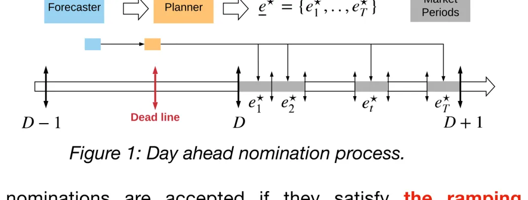
Forecaster Planner
Dead line
Market Periods
Capacity firming process
Capacity firming
The capacity firming process is decomposed into a day ahead nomination
and a real-time control process.
Figure 1: Day ahead nomination process.
|e⋆
τ − eτ−1⋆ |
Δ ≤ ΔP⋆, ∀τ ∈ 𝒯 (1)
The nominations are accepted if they satisfy the ramping power constraints
Forecaster Controller
Market Periods
Capacity firming process
Capacity firming
rn
t = πtexpetm − fe(et⋆, etm), ∀t ∈ 𝒫 (2)
For a given control period, the net remuneration of the plant is proportional
to the export minus a penalty
The penalty function depends on the specifications of the tender. In this study, is approximated as
fe(e⋆
t , etm) = πe( max (0,|et⋆ − etm| − ΔE))
2
(3)
Summary
1. Literature review
2. Capacity firming process
3. Capacity firming formulations
4. PV scenarios
5. Case study
6. Conclusions & perspectives
Capacity firming formulations: day ahead nomination
Capacity firming
The deterministic (D) objective function to minimize is
JD = ∑
τ∈𝒯
− πτexpeτ + fe(eτ⋆, eτ) (4) The stochastic (S) objective function to minimize is
JS = ∑ ω∈Ω pω ∑ τ∈𝒯 [− π exp τ eτ,ω + fe(eτ⋆, eτ,ω)] (5)
They are Quadratic Problems (QP). The D formulation uses point forecasts of PV production and the S formulation PV scenarios.
See paper submitted to PMAPS for all the equations and constraints available on orbi: https:// orbi.uliege.be/handle/2268/246270
Capacity firming formulations: real-time control
Capacity firming
The oracle assumes perfect knowledge of PV and uses nominations
Joracle = ∑
t∈𝒫
− πtexpet + fe(et⋆, et) (6)
The real-time controller (RT) uses the last PV measured value, the PV point forecasts, and nominations
Jreal−time =
∑
t∈𝒫∖{1,...,t−1}
− πtexpet + fe(e⋆
t , et) (8)
The myopic controller uses the last PV measured value and nominations
Jmyopic = − πexp
t et + fe(et⋆, et) (7)
Summary
1. Literature review
2. Capacity firming process
3. Capacity firming formulations
4. PV scenarios
5. Case study
6. Conclusions & perspectives
PV scenarios
Capacity firming
The Gaussian copula methodology has already been used to generate wind and PV scenarios in, e.g., [5]–[8].
This approach is used to sample PV error scenarios (Z) based on a point forecast model.
[5] P. Pinson, H. Madsen, H. A. Nielsen, G. Papaefthymiou, B. Klöckl, From probabilistic forecasts to statistical scenarios of short-term wind power production, Wind Energy: An Inter- national Journal for Progress and Applications in Wind Power Conversion Technology 12 (1) (2009) 51–62.
[6] P.Pinson,R.Girard, Evaluating the quality of scenarios of short-term wind power generation, Applied Energy 96 (2012) 12–20.
[7] G. Papaefthymiou, D. Kurowicka, Using copulas for modeling stochastic dependence in power system uncertainty analysis, IEEE Transactions on Power Systems 24 (1) (2008) 40–49.
[8] F. Golestaneh, H. B. Gooi, P. Pinson, Generation and evaluation of space–time trajectories of photovoltaic power, Applied Energy 176 (2016) 80–91.
PV scenarios
Summary
1. Literature review
2. Capacity firming process
3. Capacity firming formulations
4. PV scenarios
5. Case study
6. Conclusions & perspectives
The Uliège case study
Capacity firming
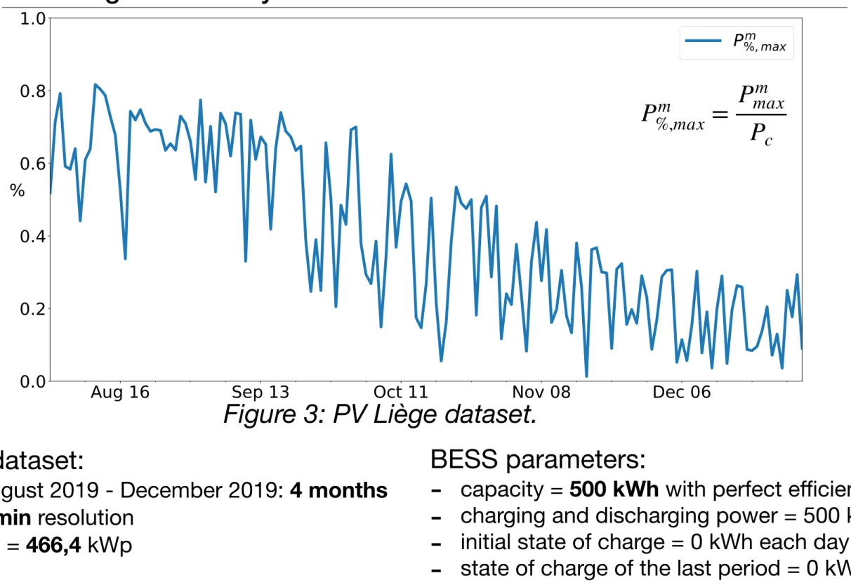
Figure 3: PV Liège dataset.
PV dataset:
-
August 2019 - December 2019: 4 months-
1 min resolution-
Pc = 466,4 kWpBESS parameters:
-
capacity = 500 kWh with perfect efficiencies-
charging and discharging power = 500 kW-
initial state of charge = 0 kWh each day -Pm %,max = P m max PcThe Uliège case study
Capacity firming
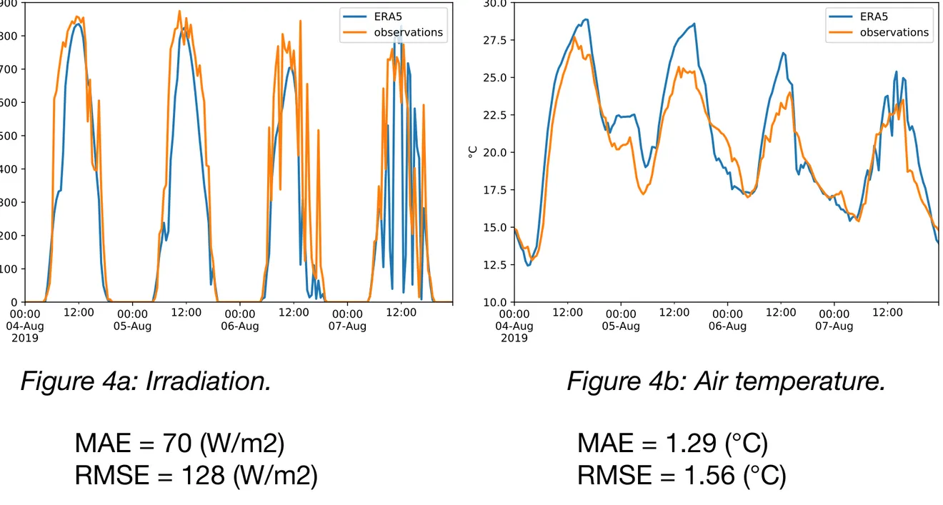
PV point forecasts are computed using the PVUSA model [10] which expresses the instantaneous generated power as a function of irradiance and air temperature according to the equation
The PVUSA parameters (a, b, and c) are estimated following the algorithm of [11]. Weather forecasts are provided by the Laboratory of Climatology of
the university of Liège, based on the MAR regional climate model [9], http://climato.be/cms/index.php?climato=fr_previsions-meteo.
[9] X. Fettweis, J. Box, C. Agosta, C. Amory, C. Kittel, C. Lang, D. van As, H. Machguth, H. Galle ́ e, Reconstructions of the 1900–2015 Greenland ice sheet surface mass balance using the regional climate MAR model, Cryosphere (The) 11 (2017) 1015–1033.
[10] R.Dows, E.Gough, PVUSA procurement, acceptance, and rating practices for photovoltaic power plants, Tech. Rep., Pacific Gas and Electric Co., San Ramon, CA (United States). Dept. of ..., 1995.
[11] G.Bianchini, S. Paoletti, A. Vicino, F. Corti, F. Nebiacolombo, Model estimation of photovoltaic power generation using partial information, in: IEEE PES ISGT Europe 2013, IEEE, 1–5, 2013.
The Uliège case study
Capacity firming
Figure 4a: Irradiation. Figure 4b: Air temperature.
MAE = 70 (W/m2) RMSE = 128 (W/m2)
MAE = 1.29 (°C) RMSE = 1.56 (°C)
The Uliège case study
Capacity firming
A set of PV scenarios is g e n e r a t e d u s i n g t h e
Gaussian copula approach
based on the PVUSA point forecasts
Red = PVUSA point forecast
Black = PV measurement Grey = 5 PV scenarios NMAE = 4.25 % NRMSE = 9.20 % ̂P i,ω = ̂Pi + zi,ω i = 1,...,r . (10)
The Uliège case study
Capacity firming
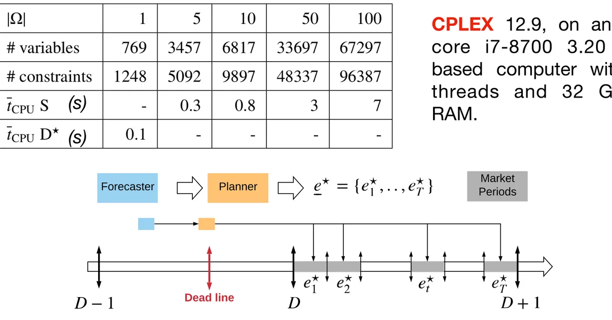
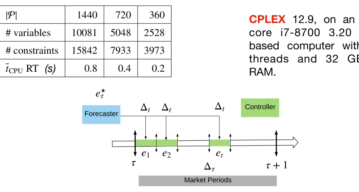
CPLEX 12.9, on an Intel core i7-8700 3.20 GHz based computer with 12 threads and 32 GB of RAM.
Table 1: Nomination average computation times.
(s) (s) Forecaster Planner Dead line Market Periods
The Uliège case study
Capacity firming
Table 2: RT controller average computation times.
(s)
Forecaster Controller
Market Periods
CPLEX 12.9, on an Intel core i7-8700 3.20 GHz based computer with 12 threads and 32 GB of RAM.
The Uliège case study
Capacity firming
ΔP⋆ = 0.5 % P c = 2.32 (kW) ΔE = 1 % PcΔτ = 5.83 (kWh) Ecap = P c = 466.4 (kW)Case study parameters
πexp = 45 (€/MWh) πe = 1 % πexp = 0.45 (€/MWh2) Δτ = 15 (min) ΔP⋆ = − (kW) ΔE = 1 % PcΔt = 0.389 (kWh) Ecap = P c = 466.4 (kW) πexp = 45 (€/MWh) πe = 1 % πexp = 6.75 (€/MWh2) Δt = 1 (min)
Nomination step Control step
Planners and controllers combinations: - D*/D/S - oracle
- D*/D/S - myopic - D*/D/S - RT
The Uliège case study
Capacity firming
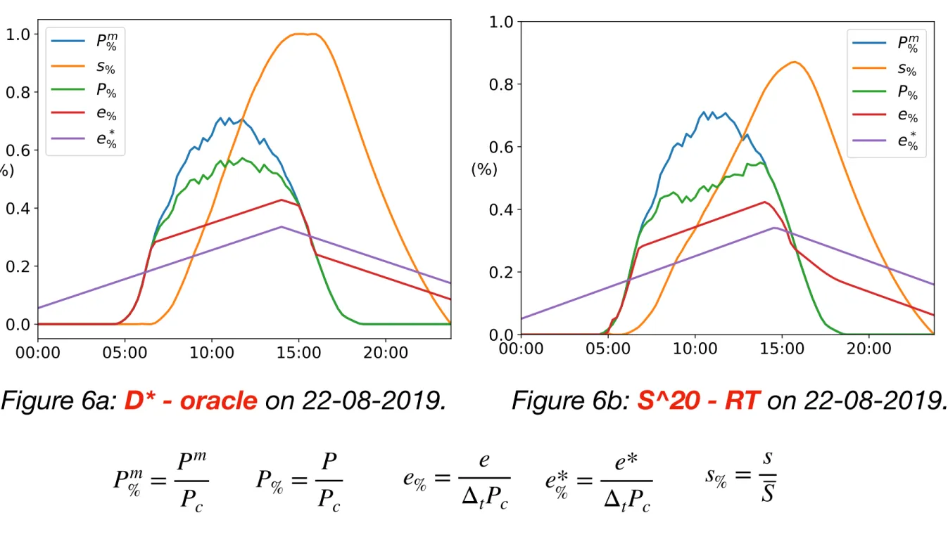
Pm % = P m Pc P% = PPc e% = eΔtPc e*% = e*ΔtPc s% = sSThe Uliège case study
Capacity firming
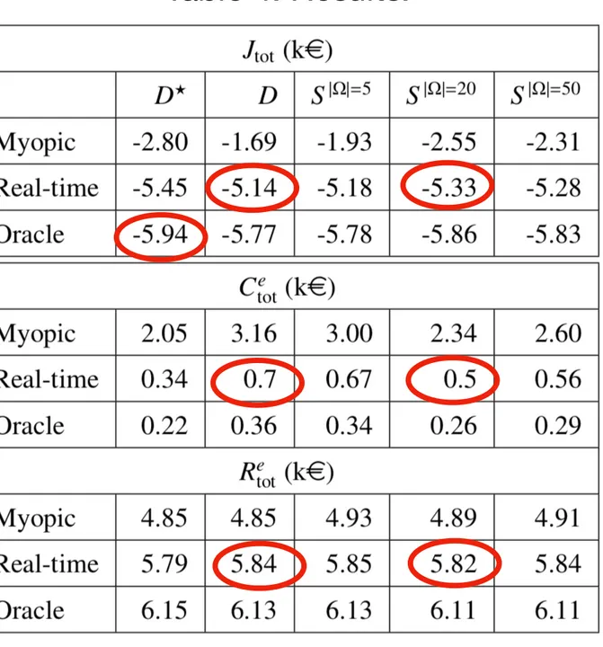
Table 4: Results.
Reference = D* - oracle
S - RT with 20 scenarios achieved 89 % of the reference. D - RT with 20 scenarios achieved 86 % of the reference.
Gross revenue of S - RT & D - RT are equivalent.
S - RT achieved smaller penalty
than D - RT.
Jtot = − Re
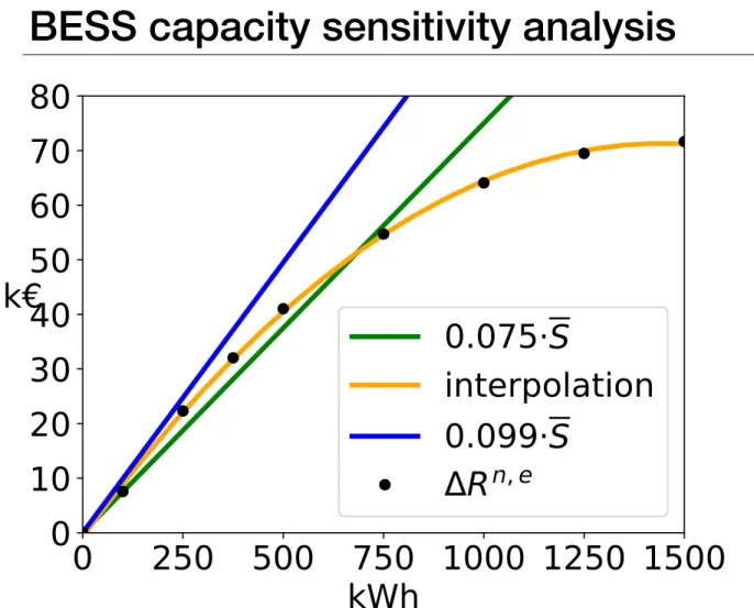
BESS capacity sensitivity analysis
Capacity firming
Inputs:
-
selling price-
BESS CAPEX-
Net revenue over 15 years for several battery capacities (0, 100, 250, 500, …) kWhOutput:
-
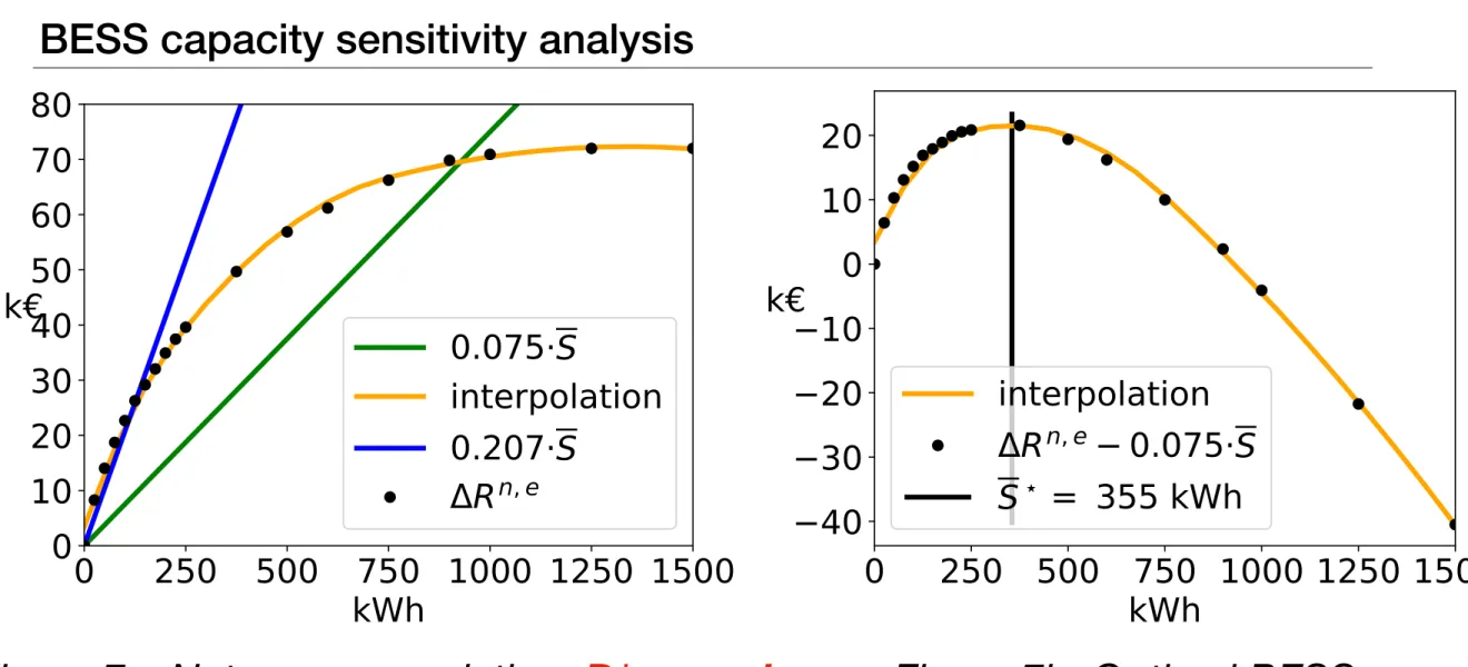
Optimal battery capacity for a given CAPEX = 0.075 (€ / kWh)Sensitivity analysis on the BESS capacity to determine its marginal value
and the optimal BESS capacity for a given BESS unit cost.
ΔRn,e
BESS capacity sensitivity analysis
Capacity firming
Figure 7a: Net revenue variation: D* - oracle. Figure 7b: Optimal BESS capacity.
D* - oracle
Optimal capacity = 355 kWh
BESS capacity sensitivity analysis
Capacity firming
Figure 8a: Net revenue variation: D - RT. Figure 8b: Net revenue variation: RT. S^20 -
D - RT
Optimal capacity = 355 kWh
Net revenue - CAPEX = 3.7 k€
S^20 - RT
Optimal capacity = 410 kWh
Conclusions
Capacity firming
The stochastic approach achieved better results than the
deterministic one.
The BESS capacity sensitivity analysis demonstrate the advantage of using a BESS to optimize the bidding day ahead strategy.
A trade-off must be found between the marginal gain provided by the
Perspectives
Capacity firming
The planner behavior should be better assessed by using at least a full year of data to fully take into account the PV seasonality.
The PV plant location should be assessed.
The non convex penalty function of the French Energy Regulatory
Commission should be considered*.
To be fully operational on the field, the controller should be able to deal with control period of one second for instance by adapting the
approach implemented in [11].
[11] J.Dumas, S.Dakir, C.Liu, B.Cornélusse, Coordination of operational planning and real-time optimization in microgrids, in: XXI Power Systems Computation Conference, 2020. Available on orbi: http://hdl.handle.net/2268/240076
Selling price calculation
Capacity firming
Inputs:
-
BESS / PV CAPEX & OPEX-
Exports for several battery capacities (0, 100, 250, 500, …) kWh Outputs:-
LCOE-
System configuration for an optimal selling priceSensitivity analysis on the BESS capacity to determine the optimal selling price related to a system configuration.