Pattern recognition with a digital holographic microscope working in partially coherent illumination

Pattern recognition with a digital holographic

microscope working in partially coherent illumination

F. Dubois, C. Minetti, O. Monnom, C. Yourassowsky, J.-C. Legros, and P. Kischel

We describe the implementation of the automatic spatial-frequency-selection filter for recognition of patterns obtained with a digital holographic microscope working with a partially coherent source. The microscope provides the complex-optical-amplitude field that allows a refocusing plane-by-plane of the sample under investigation by numerical computation of the optical propagation. By inserting a cor-relation filter in the propagation equation, the corcor-relation between the filter and the propagated optical field is obtained. In this way, the pattern is located in the direction of the optical axis. Owing to the very weak noise level generated by the partially coherent source, the correlation process is shift invariant. Therefore the samples can be located in the three dimensions. To have a robust recognition process, a generalized version of the automatic spatial-frequency-selection filters has been implemented. The method is experimentally demonstrated in a two-class problem for the recognition of protein crystals. © 2002 Optical Society of America

OCIS codes: 090.0090, 100.0100, 180.0180, 070.0070, 090.1760, 100.6740.

1. Introduction

In digital holography the interference patterns are re-corded with an electronic camera, and the holographic reconstruction is performed by numerical means.1

Several optical methods have been implemented to extract the phase and amplitude information about the object beam from the recorded interference pattern.2,3

With the phase and the amplitude information, the digital holography reconstruction simulates the optical-beam propagation by use of a discrete imple-mentation of the Kirchhoff–Fresnel propagation equa-tions. The digital holographic methods have been demonstrated in various experimental situations,4 –12

and are very promising in optical microscopy, where the three-dimensional 共3D兲 reconstruction capability overcomes the very limited depths of field due to the high magnifications.13–15 _{A very crucial point in}

dig-ital holography is that the recorded information on

the 3D scene is a two-dimensional

complex-amplitude field that can be handled as a special case of two-dimensional images. In particular, pattern-recognition methods by correlation can be imple-mented in view to detect objects that have 3D extension. This approach has been tested for the recognition of macroscopic objects having diffuse op-tical surfaces.16 _{In that case, the recorded}

holo-graphic information is related to the specific speckle field diffused by the object and the shift-invariance property of the correlation is reduced. To overcome those limitations, the recognition by correlation on the irradiance of the digitally propagated holographic data and image-processing method to reduce the speckle noise were considered.17,18 _{In this case the}

sensitivity of the correlation with respect to speckle-field phase is removed. However, it has been shown that the signal phase contains crucial information.19

Therefore the phase should be kept to achieve the full capabilities of pattern recognition in digital hologra-phy. In this contribution, we investigate the recog-nition by correlation of full complex-amplitude fields obtained by a digital holographic microscope. Holo-graphic setups often use laser sources that avoid any coherence problems in interferometer configuration. However, highly coherent beams are very sensitive to the microstructure of the sample and to any defect in the optical paths. As a result, the complex ampli-tudes are deeply affected by the coherent noise that severely reduces the optical quality.20 _{To alleviate}

such problems, our microscope uses a partially coher-ent source.

F. Dubois 共frdubois@ulb.ac.be兲, C. Minetti, O. Monnom, C. Yourassowsky, and J.-C. Legros are with the Universite´ Libre de Bruxelles, Microgravity Research Center, 50 Avenue F. Roosevelt, CP165兾62, B-1050 Brussels, Belgium. P. Kischel is with the Laboratoire de Biologie Mole´culaire et Ge´nie Ge´ne´tique, Alle´e de la Chimie, 3, Campus du Sart-Tilman, Baˆt. B6, 4000 Liege 1, Bel-gium.

Received 9 November 2001; revised manuscript received 18 March 2002.

0003-6935兾02兾204108-12$15.00兾0 © 2002 Optical Society of America

The microscope set up and the related optical methods are described in Section 2. To implement the recognition process by correlation for digital ho-lographic signals, an impressive set of filter-computation algorithms is available in the literature. Those methods overcome the classical limitations of the matched filters.21 _{With the synthetic}

discrimi-nant function共SDF兲 algorithm,22_{the filters are}

com-puted as linear combinations of reference patterns to give a priori fixed central-correlation intensities or responses when they are correlated with the refer-ence images. This algorithm has played a central role in making the recognition invariant to input dis-tortions. Adding minimization criteria to the SDF central-correlation constraints made further signifi-cant improvements. The minimization of the mean square variance for input images corrupted by noise,23_{and the minimization of the average}

correla-tion energy24,25共MACE兲 have been used to optimize,

respectively, the signal-to-noise ratio共SNR兲 and the peak sharpness. Methods have been also

success-fully proposed to globally optimize several

criteria.26 –28 _{It has been also demonstrated that}

nonlinear transforms applied in the Fourier plane can significantly improve the discrimination, and the correlation noise robustness,29 –31 _{and that this}

method can be applied when distortion invariance is requested.32 _{Critical reduction of the correlation}

height occurs when the targets are surrounded by noise or by clutter. This problem has been consid-ered and elegant solutions based on the decision the-ory33,34_{or on a minimization of mean square error}35

have been proposed. To make the recognition insen-sitive to the input distortions, we developed the auto-matic spatial frequency selection 共ASFS兲 algorithm that involves reference images and distorted versions of them to select the significant spatial frequencies36 –38

in the recognition process. The implementation of the correlation in the digital holographic process is de-scribed in Section 3. The ASFS method is described in Section 4, where the changes to be used with digital holographic amplitudes are outlined. With the ASFS algorithm, the central-correlation amplitudes between the reference images and the filter are constrained to give a priori set values, and a cost function depending on the reference and distorted images is minimized. This function is called the ASFS cost function.

In Subsection 5.A, we describe the implementation of a two-class recognition process based on images extracted from an actual application in protein crys-tallization monitoring. Some information about the experimental system is given at the beginning of this section. In Subsection 5.B, the recognition results are provided, and it is shown that the system keeps the shift-invariant property and is able to recognize objects in depth. Concluding remarks are reported in Section 6.

2. Digital Holographic Microscope Working with a Partially Coherent Illumination

The optical setup is very similar to the one described in detail in Ref. 14, and we give here only a short

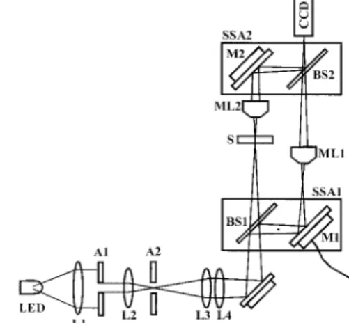
description. The microscope is implemented in a Mach–Zehnder interferometer共Fig. 1兲. A red light-emitting diode 共LED兲 of 4 mW at 660 nm with a spectral width of 20 nm is used as an incoherent optical source. A secondary partially coherent source is achieved by imaging the LED-emitting sur-face with an optical filtering system. The collimated beam by the first lens共L₁—focal length f₁, is filtered by an aperture共A1兲 of diameter ␳ that increases the

spatial-coherence width of the source image in the back focal plane of the second lens共L2—focal length

f₂兲. A third lens 共L₃兲 collimates the beam and the

lens共L4兲 images the aperture A2 in the sample

vol-ume 共S兲. The interferometer is constituted by two sub-system assemblies共SSA兲. Each SSA includes a beam splitter 共BS兲 and a mirror 共M兲. Microscope lenses 共10⫻兲 are placed in both the object and the reference beams. The image planes of these two mi-croscope lenses 共ML兲 are interfering on the input plane of the CCD camera sensor located after the beam combiner共BS2兲. The partial coherence width

of the secondary source is kept with a magnification ratio given by f4兾f3, where f4 and f3 are the focal

lengths of the lenses L₄ and L₃. The experimental volume is placed in the beam waist of the lens L4in

such a way that it is assumed that the sample共S兲 is illuminated in plane waves. Indeed, the illumina-tion wavefront of the sample can be considered as plane if the thickness of the sample is smaller than 2␭f₂2_f

4 2_兾␳2_f

3

2 _{共see Ref. 14兲. In our system, f} 2 ⫽ 50

mm, f3⫽ 200 mm, f4⫽ 200 mm and ␳ ⫽ 0.25 mm, the

thickness has to be smaller than 52 mm. We dem-onstrated that the partial coherence nature of the source limits the digital holographic refocusing dis-tance d according to the following inequality14_:

d⬍⬍ 2f2f4

␳f3␯max

, (1)

where ␯max denotes the maximum expected spatial

frequency.

For refocusing distance around the best-focus ob-ject plane higher than this limit, the resolution of the

Fig. 1. Scheme of the microscope implemented in a Mach– Zehnder interferometer with a spatially partial coherent source.

reconstructed image is progressively reduced. The main advantages in using a partially coherent source are the speckle removal, the influence reduction of perturbations that are located at a distance d larger than the one expressed by the inequality of Eq. 共1兲, and the suppression of multiple reflection interfer-ences. We have a magnification ratio of 10 fixed by the microscope lenses. Thus 0.86 ␮m of the input scene matches the CCD pixel size of 8.6␮m. There-fore␯_maxis estimated equal to 106_{兾m and d has to be}

smaller than 400 ␮m. For refocusing distances higher than this limit, the resolution of the recon-structed image is progressively reduced. As the dig-itized images共256 levels兲 have 512 ⫻ 512 pixels, the field of view of the system is approximately 440␮m ⫻ 440␮m.

The mirror M1is mounted on a piezoelectric

trans-ducer to implement the phase-stepping technique. The modulo 2␲ phase ␾共s, t兲, where 共s, t兲 are the discrete spatial variables, is computed from four␲兾2 phase-shifted fringe images I1 to I4 with the

four-frames algorithm:

␾共s, t兲 ⫽ tan⫺1

冋

I1共s, t兲 ⫺ I3共s, t兲

册

. (2)

The modulus of the amplitude of the optical field is calculated as the square root of the object intensity distribution.

3. Digital Holographic Reconstruction and Correlation Implementation

The object path of the optical system described in the previous section performs the image of the light dis-tribution of the focused plane P that is crossing the experimental volume of the sample. As the interfer-ence patterns between the object and the referinterfer-ence beams are recorded with a phase-shifting capability, the complex amplitude in the focused plane is com-pletely determined. Thanks to this information, we want to compute the optical field in planes that are parallel to P, the focused plane, and that are also crossing the sample. The amplitude distribution in a plane P⬘ parallel to P and separated by a distance d along the optical axis is computed by the Kirchhoff– Fresnel propagation integral in the paraxial approx-imation,39 u0共 x⬘, y⬘兲 ⫽ exp共ikd兲

再

冋

册

冎

where u_i共x, y兲 is a complex optical field in P, u₀共x⬘, y⬘兲 is the complex optical field in P⬘, ␭ is the wavelength,

k⫽ 2␲兾␭, 共x, y兲, 共x⬘, y⬘兲 are the spatial variables, 共␯_x, ␯y兲 are the spatial frequencies, j ⫽ 公⫺1, and

F_{共C兲␣␤}⫾1g共␣, ␤兲 denotes the direct or inverse

two-dimensional continuous Fourier transformations de-fined by F_{共C兲␣␤}⫾1g共␣, ␤兲 ⫽

兰

兰

For digital reconstruction, Eq.共3兲 is implemented in a discrete form. The sampling distance is⌬ in both

x and y directions. The discrete form of Eq. 共3兲 is written by

u0共s⬘⌬, t⬘⌬兲 ⫽ exp兵 jkd其FU,V⫺1exp

冋

⫺jk␭2_d

2N2_⌬2 共U 2

⫹ V2_兲

册

s,t⫹1ui共s⌬, t⌬兲, (5)

where N is the number of pixels in both directions and s, t, s⬘, t⬘, U and V are integer numbers varying from 0 to N⫺ 1. F⫾1denotes the direct and inverse Fourier transformation defined by

Fk,l⫾1g共m, n兲 ⫽ 1 N k,l

兺

冋

册

where k, l, m, n are integers in such a way that k, l,

m, n ⫽ 0, . . . , N ⫺ 1. The optical quality of the

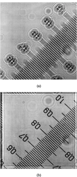
refocusing is shown on a microscopic scale by Figs. 2共a兲 and 2共b兲. The image of Fig. 2共a兲 is the intensity distribution recorded with a defocus distance of 400 ␮m. Figure 2共b兲 shows the refocusing by digital ho-lography. In the following, there is no need to

con-sider amplitude distributions depending on

continuous space and spatial frequencies variables 共x, y兲, 共␯x,␯y兲. Therefore we simplify the notations

by considering sampled amplitude distributions de-pending on integer spatial variables. In the spatial domain, the sampled amplitude distributions will be noted by the lower case letters x共s, t兲, y共s, t兲, and h共s,

t兲, where s, t are integers 共s, t ⫽ 0, . . . , N ⫺ 1兲 and h

represents a correlation filter as defined below. The corresponding amplitude distributions in the spatial-frequency domain are denoted by the corresponding uppercase letters X共U, V兲, Y共U, V兲, and H共U, V兲. Thanks to these notations, Eq.共5兲 can be rewritten as

x0共s⬘, t⬘兲 ⫽ exp兵 jkd其FU,V⫺1exp

冋

⫺jk␭2_d 2N2_⌬2 共U 2 ⫹ V2_兲

册

The correlation product共x₀ R h兲共s⬘, t⬘兲 between a filter h共s, t兲 and an input amplitude distribution x0共s,

t兲 is achieved by computing:

共 x0丢 h兲共s⬘, t⬘兲 ⫽ FU,V⫺1H*共U, V兲 X0共U, V兲, (9)

where the superscript * denotes the complex conju-gate. By combining Eq.共7兲 and Eq. 共9兲, the correla-tion product between propagated amplitude x0共s, t兲 by

digital holography and a filter h共s, t兲 is expressed by 共 x0丢 h兲共s⬘, t⬘兲 ⫽ exp兵 jkd其FU,V⫺1H*共U, V兲

⫻ exp

冋

册

Equation共10兲 shows that the correlation product of the refocused amplitude plane with a correlation fil-ter is achieved by introducing, as a multiplicative field, the complex conjugate of the filter amplitude in the digital holographic Eq.共7兲. The next section is devoted to the computational method of the correla-tion filters.

4. Automatic Spatial Frequency Selection Algorithm to Compute Pattern Recognition Filters for Digital Holographic Patterns

The ASFS algorithm that has been developed to com-pute correlation filter for image recognition33_{can be}

applied for complex amplitude patterns obtained in digital holography with only a few changes. As for many other correlation algorithms, the ASFS filter is computed thanks to a set of typical patterns that have to be representative of the application. For example, if we want to recognize a specific object that can be rotated, the designer will select a set of images representing the object with different orientations. It is also necessary to add patterns that have to be unrecognized. In our example, those could be im-ages of objects that we want to reject. On the basis of those images, a correlation filter is computed by the ASFS algorithm in such a way that images to be recognized will give rise to important intensity cor-relation peaks while images to be rejected will only give low-level intensities. In its simplest way, the recognition is based on the correlation-peak inten-sity. We consider a two-class problem where the patterns to be rejected are placed in a set of patterns called class 0 and all patterns to be recognized are placed in a second set called class 1. We want to realize a unique filter h共s, t兲 that is able to discrimi-nate the patterns of class 1 with respect to the pat-terns of class 0. The generalization to multiple filters is obvious. On the basis of the pattern-recognition problem, reference images xkq共s, t兲 are

selected where k is the class number共k ⫽ 0, 1兲 and q is the image number in the class k关q ⫽ 0, . . . , Q共k兲 ⫺ 1, where Q共k兲 is the number of pattern of the class k兴. It is also assumed that the total number of reference images is T. Filter h共s, t兲 has to give a set of re-sponses rkqdefined by the user that are the

correla-tion amplitudes located at 共0, 0兲 when the filter is correlated with xkq共s, t兲. In the Fourier space, it is

expressed by

rkq⫽

兺

n⫺1

H*共U, V兲 Xkq共U, V兲. (11)

As the number of pixels is larger than the number of reference images, Eq.共11兲 does not completely de-termine the filter components. Therefore an addi-tional constraint can be imposed to reduce the side-lobe energies. For this purpose a set of distorted images y_kqi共s, t兲 is associated with each reference im-age xkq, where i ⫽ 0, . . . , Ikq ⫺ 1, and Ikq is the

number of distorted patterns corresponding to x_kq共s,

t兲. The ykqi共s, t兲 images are chosen in the definition

step of the pattern recognition problem. As an

ex-Fig. 2. Refocusing by digital holography on a metric scale共100 divisions兾mm兲. 共a兲 Image of the defocused intensity. 共b兲 Image of the computer refocused intensity. The refocus distance is 400 ␮m.

ample, if the patterns to be recognized can be rotated,

y_kqi共s, t兲 images will be slightly rotated versions of xkq共s, t兲. The ASFS constraint minimizes, in

aver-age, the contributions of the spatial frequencies, where the components between Xkq共U, V兲 and Ykqi共U,

V兲 are significantly different. It is requested that

the following expression be minimized:

F⫽

兺

U,V⫽0 N⫺1

兺

k,q,i

兩 H*共U, V兲兵Xkq共U, V兲 ⫺ Ykqi共U, V兲其兩2

(12) The ASFS filter is computed by imposing the Eq. 共11兲 and by minimizing Eq. 共12兲. By lexicographi-cally scanning H共U, V兲, Xkq共U, V兲, and Ykqi共U, V兲 to

make column vectors H, Xkqand Ykqi, and by

order-ing vectors Xkqside-by-side, we build the X matrix.

Eq.共11兲 is rewritten by the following matrix equation:

X⫹H⫽ r, (13) where the superscript⫹denotes the Hermitian con-jugate operation r is the column vector that involves the response elements r_kq with the same ordering sequence as for matrix X.

The ASFS cost function of Eq.共12兲 is rewritten in a matrix form:

F⫽ H⫹EH. (14)

E is an N2_{⫻ N}2_{diagonal matrix defined by}

E共Z, Z兲 ⫽

兺

k,q,i

兩 Xkq共Z兲 ⫺ Ykqi共Z兲兩2, (15)

where Xkq共Z兲 and Ykqi共Z兲 are the Zth components of

vectors Xkqand Ykqi. Vector H, which verifies Eq.

共13兲 and which minimizes Eq. 共14兲, is obtained by use of the method of the Lagrange multipliers24 _{and is}

expressed by

H⫽ E⫺1X共X⫹E⫺1X兲⫺1r. (16) Equation共16兲 is the solution of the ASFS filter.

The difference between the ASFS filters computed for digital holography and the ones for image process-ing is the full complex nature of the patterns x_kq共s, t兲 and ykqi共s, t兲. For this reason, in the following xkq共s,

t兲 and y_kqi共s, t兲 will be called reference fields and

distorted fields instead of reference and distorted im-ages. It is also for this reason that the matrix 共X⫹_E⫺1_X兲⫺1 _{is a complex matrix instead of a real}

symmetric one.

5. Implementation of a Pattern-Recognition Problem

A. Statement of the Problem

The pattern-recognition problem that we selected comes from an actual application in protein crystal growth. The reason why the protein crystal growth is a crucial issue is summarized as follows: The bio-chemical properties of a protein are mainly defined by its reactive sites and its atomic structure. The reactive-sites and the atomic-structure information are obtained by x-ray diffraction analysis of the

pro-tein crystals. Owing to the structural complexity of proteins, the physical-chemical processes governing the crystallization of protein are badly or not at all known, obliging biochemists to use empirical meth-ods. That means that they have to perform many crystallization processes with small changes of the experimental parameters before achieving success. As the crystal quality is first assessed by long optical-microscopy observations, there is an important need in automatic methods to monitor protein-crystal-growth processes. In this way, the digital holo-graphic microscope gives access to the localization of crystals in solution while the pattern-recognition techniques are intended to identify and track each crystal during growth. In our experiments, we use a lysozyme protein for the crystallization process. Our crystallization cells have an experimental vol-ume surrounded by two parallel optical plates

sepa-rated by an internal distance of 800 ␮m.

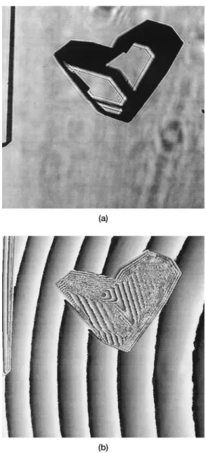
Crystallization of the lysozyme protein solution, used at a concentration of 100 mg兾ml⫺1, was initiated with a precipitating solution composed of sodium chloride 共20% w兾v, pH 4.5兲. Both precipitating and protein solutions were cast with 1%共w兾v兲 low melting aga-rose gel共SeaPlaque Agarose, Cambrex兲 above the gel-ling point 37 °C. The lysozyme gel was poured over the gelled precipitating solution. Owing to the dis-tance between the optical windows, the growing crys-tals can be largely out of focus. In the example of the pattern-recognition problem that we tested, we want to reject the crystal shown by Figs. 3共a兲 and 3共b兲 共Crystal 0兲 and to recognize the crystal 共Crystal 1兲 shown by the Figs. 4共a兲 and 4共b兲. Those pictures have been recorded when the crystals are focused by the imaging channel of the microscope. The phase images Figs. 3共b兲 and 4共b兲 are digitized on 256 levels. The actual phase value in one point is obtained by multiplying the corresponding gray level by the con-stant 2␲兾255. In the phase images shown by Figs. 3共b兲 and 4共b兲, we observe that the background phases around the crystals are not uniformly distributed ow-ing to two types of optical defects. The optical win-dows of the experimental cell are not completely flat and are not exactly parallel to each other. There is also a small misalignment of the interferometer. Those optical defects have to be taken into account as they are introducing distortions and shifts on the Fourier transformations of the complex amplitudes during the correlation process. Therefore if no care is taken for that, we could expect significant mis-alignment between the Fourier-transformed input amplitude and the pattern-recognition filter. This problem was identified a long time ago as a critical one in optical implementation of the correlation.40

We could think that those defects could be removed by using higher-quality experimental cells and by adjusting the interferometer in a better way. How-ever, this approach is not realistic from a practical point of view because large-scale experiment batches request cheap experimental cells that present signif-icant deviations with respect to perfect flatness and thickness. We apply a phase correction on all the

complex-amplitude fields that we are recording be-fore any further processing. This is applied to the amplitude fields used to compute the correlation filter and for any amplitude fields recorded during the rec-ognition process. Let us call␾共s, t兲 the phase of the complex amplitude x共s, t兲, and ␾B共s, t兲 the phase of

the background complex amplitude x_B共s, t兲 measured with the cell without a sample. The corrected phase ␾c共s, t兲 is obtained by computing:

␾c共s, t兲 ⫽ mod2␲关␾共s, t兲 ⫺ ␾B共s, t兲兴. (17)

The corrected phase map corresponding to Fig. 4共b兲 is shown by Fig. 5. In the application that we foresee, the phase-map correction is not really a problem. Indeed, before we begin an experimental crystal growth process, the phase map of the cell can be recorded as a background phase map used to correct the complex-amplitude fields during the process.

That can be also made with a set of background phase maps if the cell has to be laterally moved to monitor a larger area of the experimental cell. In our tests, we observed that the phase distortions in the cell itself due to the growing process could be neglected in such a way that a phase-correction map can be used during a complete growing process. Let us now de-scribe how the reference-field sets have been consti-tuted. For the first time, we formed two complex-amplitude fields that we called primary-reference fields. They are formed according to the following operations. The intensity and corrected-phase im-ages of the crystals in Figs. 3 and 4 have been cropped and centered in constant intensity and a phase back-ground of 512⫻ 512 pixels. The constant intensity and the phase-background levels have been com-puted by averaging the intensities and corrected phases in a 20 ⫻ 20 window located in the back-ground regions. The results of these processes for

Fig. 3. _{共a兲 Intensity image and 共b兲 phase image of the crystal to be} rejected.

Fig. 4. 共a兲 Intensity image and 共b兲 phase image of the crystal to be recognized.

the crystal of Fig. 4 are shown by the Figs. 6共a兲 and 6共b兲. We denote the intensity fields corresponding to the images in Figs. 3共a兲 and 4共a兲 by I0共s, t兲 and I1共s, t兲

and the corresponding corrected-phase fields by␾0共s,

t兲 and ␾1共s, t兲. The primary-reference fields are

ob-tained by computing:

xk共s, t兲 ⫽

冑

where k⫽ 0, 1.

From each xk共s, t兲, we build six reference fields

x_kq共s, t兲 by in-plane rotating x_k共s, t兲 around the center

point共s, t兲 ⫽ 共255, 255兲 according to:

xkq共s, t兲 ⫽ R关⫺10° ⫹ q.4°兴xk共s, t兲, (19)

where the integer q⫽ 0, . . . , 5 and R关␣兴 denotes the rotation operation by an angle␣. To each reference pattern xkq共s, t兲 is associated with a single distorted

pattern ykqi共s, t兲 in such a way that:

ykqi共s, t兲 ⫽ R关2°兴 xkq共s, t兲 (20)

because we have a single distorted field by reference field. In this case i⫽ 0.

The reasons why the selected distortions to com-pute the filter are from the in-plane rotation can be summarized as follows: The recognition of the

pro-tein crystal is a milestone of a wider objective that is the monitoring of growing crystals. For this pur-pose, pattern recognition will be used as a tracking tool that will allow us to identify and to follow several crystals in time. For each crystal, this objective re-quires the implementation of an iterative sequence of several processes including pattern recognition, post-segmentation to crop the crystal fields, and compu-tation of a new pattern-recognition filter to be ready for a new identification later. Therefore the shape of each crystal is expected to change between two re-cordings in such a way that pattern recognition has to be robust with shape changes. The changes that can be expected are shifts, in-plane兾out-of-plane rota-tions 共when the crystals are growing in a solution instead of a gel兲, and growing. Growing can be anisotropic and very complex when crystal defects

appear. Therefore prediction of these shape

changes is not obvious and the most realistic way to handle this problem is to select an image-acquisition rate that guarantees small shape changes between two consecutive image acquisitions. In that context, small plane rotation as a distortion model in-creases the robustness of the recognition process due to the spatial-frequency selection obtained by the minimization of Eq.共12兲. The number of reference and distorted fields and the incremental angles be-tween the reference fields can of course be optimized in view of a practical application. However, the scope of this article is not to address this problem: that will be the topic for a future work. Because of the fields x_kq共s, t兲 and y_kq共s, t兲, the filter H共U, V兲 is computed according to Eq. 共16兲. The filter compo-nents H共U, V兲 are scaled in such a way that the response-1 correlation peaks give rise to correlation-peak intensities equal to 255 in the center of the correlation plane when they are correlated with the reference fields to be recognized.

B. Pattern Recognition Tests

The first objective of the tests is to demonstrate that the pattern-recognition system, combining correla-tion and digital holographic reconstruccorrela-tions, is able to recognize the crystal of Figs. 4共a兲 and 4共b兲 and to reject the crystal of Figs. 3共a兲 and 3共b兲 even when the input fields are recorded out of focus in the micro-scope channel. If there is some defocus distance D between the reference fields used to compute the fil-ter and the input field, it is expected that a recogni-tion correlarecogni-tion peak is happening when the digital holographic reconstruction distance of Eq.共10兲 is d ⫽

D. Conversely, by scanning the reconstruction dis-tance d in Eq.共10兲, it is expected that we will observe a peak formation in depth with a maximum when the reconstruction distance d corresponds to the defocus distance D. The second objective is to test the shift-invariance property of the recognition process. In-deed, with respect to the pattern-recognition methods developed for image processing, we must work with important phase information directly recorded with the input images and we must check that the

exper-Fig. 5. Phase-corrected image of the crystal of Fig. 4共b兲.

Fig. 6. Central region of the primary reference共a兲 intensity image and共b兲 phase image of the crystal to be recognized.

imental process does not disturb it too much for the pattern-recognition operation.

To test these two aspects, we recorded intensity images and phase maps of the two crystals in two different lateral positions共displacement perpendicu-lar to the optical axis兲 and for 10 defocus distances by changing, with mechanical translation stages, the po-sition of the experimental cell in the sample place of

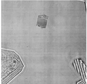
the microscope. Those images are sorted in four se-ries according to the crystal number and the lateral position in the field of view. The series are labeled as follow: series 1共crystal 0兾lateral position 1兲, se-ries 2共crystal 0兾lateral position 2兲, series 3 共crystal 1兾lateral position 1兲 and series 4 共crystal 1兾lateral position 2兲. Note that each series involves different defocus distances D of the same sample in the same position. The intensity and phase images were re-corded without any processing of the background to operate in actual experimental conditions. The po-sitions of the crystals with respect to the frame center are for the series 1, 2, 3, and 4, respectively,共50, 85兲, 共⫺49, ⫺93兲, 共⫺8, ⫺122兲, and 共167, ⫺115兲. The defo-cus distances that are considered for the four series cover a range of 225␮m and start from ⫺150 ␮m up to 75␮m in steps of 25 ␮m. It has to be emphasized that a classical optical microscope with such magni-fication共⫻10兲 has a typical depth of focus of 10 ␮m. A defocused intensity image共the crystal of Fig. 4兲 by a distance of 150␮m is shown in Fig. 7 and it can be compared with the best focused image shown by Fig. 4共a兲. A correction-phase step has been applied with a single background phase for each series to keep a realistic experimental protocol. With the intensity images and the corrected phase images, the complex-amplitude fields were computed for all the images of

Fig. 7. Defocused image by a distance of_{⫺150 ␮m.}

Fig. 8. Correlation intensities for the crystal to be recognized共a兲 series 3 and共b兲 series 1. Defocus distance 100 ␮m, reconstruction distance 100␮m.

Fig. 9. Horizontal correlation-intensity profile crossing the corre-lation peak as a function of the digital holographic reconstruction distance d共a兲 series 3 and 共b兲 series 4. Defocus distance D ⫽ 0 ␮m.

the four series. Correlation tests have been per-formed on the complete set of fields of the four series. The 3D plots of Figs. 8共a兲 and 8共b兲 show the correla-tion intensities when the filter is respectively corre-lated with the fields of series 3 and series 1, when the defocus distance D is in both case equal to 100␮m,

and the reconstruction distance d ⫽ 100 ␮m. We observe in those plots that the correlation gives rise to quite-higher intensity levels for the crystal that has to be recognized. The recognition peak is also narrow and well shaped. We observe also that the maximum correlation peak is lower than the level of 255 constrained during the filter computation. This is due to the fact that the input field originates now from a real experimental process and not a reference field used to compute the filter. The 3D plots of Figs. 9 and 10 show, for the four series, the evolution of the horizontal correlation-intensity profile crossing the center of the crystal position共defined by the position of the reference fields兲 for various reconstruction dis-tances d of Eq. 共10兲. In the recognition cases, we observe that the correlation-intensity profiles have a well-shaped maxima for d values very similar to D and that the intensity peak is sensitive with respect to the reconstruction distance d. Plots of Figs. 11 and 12 represent, for all the input fields of the four series, the evolution of the maximum correlation in-tensities as a function of the digital holographic re-construction d. As expected, we observe that we obtain the maximum correlation intensities at recon-struction distances that correspond, within the accu-racies of our mechanical translation stage, to the defocus distances of the recorded input images. We observe, also on these plots, similar results for the series 3 and 4 indicating that the system presents a good shift invariance property. Figure 13 shows the defocus distance D as a function of the reconstruction distance d when the correlation intensity has a max-imum 共series 3兲. Within the accuracy of our me-chanical translation stage, we obtain a good linearity between d and D, and a very small systematic error probably due to our mechanical translation stage. For the higher defocus distances D in series 3 and 4, a low decrease of the correlation-peak height can be seen. The intensities corresponding to series 1 and 2 are quite lower and are almost identical for every

Fig. 10. Horizontal correlation intensity profile crossing the cor-relation center as a function of the digital holographic reconstruc-tion distance d_{共a兲 series 1 and 共b兲 series 2. Defocus distance D ⫽} 0_␮m.

distance d. Therefore, we can apply a decision-threshold level that correctly discriminate the results obtained with series 1 and 2 and series 3 and 4. It can be objected that the recognition problem that we consider is obvious as the crystal shapes shown by Figs. 3 and 4 are very different. Indeed, a tracking application would include a priori during any filter computation process a crystal to be recognized and a set of crystals to be rejected. To estimate the behav-ior of the pattern-recognition process with

non-training crystal samples, we measured the

correlation-peak intensities for a set of 25 different fields that were not involved in the training set for the filter computation. As result, we have an aver-age maximum correlation intensity of 64.30 with a standard deviation of 13.40, indicating a good dis-crimination of the process for the recognition of the

crystal of Fig. 4. According to Eq. 共19兲, the ASFS filter is computed to be robust with respect to in-plane rotations over a range of关⫺10°, 10°兴 with respect to the crystal orientations shown by Figs. 3 and 4. We tested this robustness by computing the intensities of the correlations between the filter and the in-plane rotated amplitude fields of the focus phase-corrected amplitudes corresponding to the crystals shown by Figs. 3 and 4. The results are shown by Fig. 14 where the maximum correlation intensities are rep-resented as a function of the in-plane rotation angle by a step of 1° in the range关⫺15°, 15°兴. We obtain two curves. The highest one corresponds to the am-plitude fields to be recognized and the lowest one is obtained with the fields to be rejected. We observe that the intensity levels are quite different for the two

Fig. 12. Maximum correlation intensities as a function of the digital reconstruction distance d for the samples of series 2 and 4.

Fig. 13. Defocus distance D as a function of the reconstruction distance d when the maximum correlation intensity is reached for the samples of series 3.

Fig. 14. Maximum correlation intensities between the ASFS fil-ter and the in-plane rotated amplitude fields of the focus phase-corrected amplitudes corresponding to the crystals shown in Figs. 3 and 4.

types of fields and that the fields to be recognized give rise to high-intensity levels for the orientations in the range of 关⫺15°, 15°兴 demonstrating that the ASFS filter responses are in agreement with the constraints imposed during the filter computation.

6. Concluding Remarks

This contribution describes a way to introduce pattern recognition by a correlation process on complete am-plitude distributions produced by a digital holography microscope. In order to reduce the noise inherent to the laser source, we are using a digital holographic microscope that takes advantage of a partially coher-ent source. The ASFS algorithm has been imple-mented to compute the correlation filter. Owing to the low level of noise produced by the partially coher-ent source, the full amplitude of information of the input field is kept for the recognition process. How-ever, the need of phase correction on every input pat-tern is identified. The pattern recognition by correlation on amplitude fields provided by the digital holographic setup is tested on a two-class problem for the recognition of protein crystals. It is shown that the system keeps the shift-invariance property of the usual correlation and that the maximum correlation peak occurs when the defocus distance of the object is equal, within the experimental errors, to the digital holographic reconstruction distance. Therefore the system is able to locate objects in depth when they are out of focus with respect to the imaging channel of the microscope. Future studies will be oriented toward the development of the automatic tracking of growing crystals for the implementation of an automated ap-plication. The implementation of the automated tracking system will be carefully studied as we can expect, owing to the growing process, to measure large phase changes between two consecutive hologram re-cordings of the same crystal. The basic concept of the tracking system is to compute, for each crystal, with a time delay⌬t, a correlation filter based on a few pre-viously recorded digital holograms for recognition. If the time delay is too long, the amplitude field of a crystal will be changed too much with respect to the previously recorded amplitude fields to enable a reli-able recognition. Therefore the tracking will be im-plemented by adequately choosing the acquisition frequency of the digital holograms.

This research is supported by the Walloon Region Research Program “Recherche d’initiative” under the

MICADO contract 001兾4512. The authors are

grateful to J. Becker from the European Space Agency who provided us the results of the pioneer works on digital holography obtained by B. Skarman.

References

1. U. Schnars and W. Ju¨ ptner, “Direct recording of holograms by a CCD target and numerical reconstruction,” Appl. Opt. 33, 179 –181共1994兲.

2. K. Creath, “Temporal Phase Measurement Methods,” in

Inter-ferogram Analysis: digital fringe pattern analysis, D. W.

Rob-inson and G. T. Reid, eds. 共Institute of Physics, Publishing Ltd., London, 1993兲, pp. 94–140.

3. I. Yamaguchi and T. Zhang, “Phase-shifting digital hologra-phy,” Opt. Lett. 22, 1268 –1270_共1997兲.

4. B. Skarman, K. Wozniac, and J. Becker, “Simultaneous 3D-PIV and temperature measurement using a New CCD based holographic interferometer,” Flow Meas. Instrum. 7, 1– 6 共1996兲.

5. T. M. Kreis, W. P. O. Ju¨ ptner, “Principle of digital holography,” in Fringe ’97: Automatic Processing of Fringe Patterns, W.

Jæptner and W. Osten, eds.共Wiley, New York, 1998兲, pp. 353– 363.

6. B. Nilsson and T. E. Carlsson, “Direct three-dimensional shape measurement by digital light-in-flight holography,” Appl. Opt.

37, 7954 –7959共1998兲.

7. E. Cuche, F. Bevilacqua, and C. Depeursinge, “Digital holog-raphy for quantitative phase contrast imaging,” Opt. Lett. 24, 291–293_共1999兲.

8. D. O. Hogenboom, C. A. Dimarzio, T. J. Gaudette, A. J. Dev-aney, S. C. Lindberg, “Three-dimensional images generated by quadrature interferometry,” Opt. Lett. 23, 783–785_共1998兲. 9. M. Adams, T. M. Kreis, and W. P. O. Ju¨ ptner, “Particle size and

position measurement with digital holography,” in Optical

In-spection and Micromeasurements II, C. Gurecki, ed., Proc.

SPIE 3098, 234 –240共1998兲.

10. E. Cuche, F. Belivacqua, and C. Despeuringe, “Digital holog-raphy for quantitative phase-contrast imaging,” Opt. Lett. 24, 291–293共1999兲.

11. B. Javidi, E. Tajahuerce, “Encrypting three-dimensional infor-mation with digital holography,” Opt. Lett. 39, 6595– 6601 共2000兲.

12. F. Dubois, L. Joannes, O. Dupont, J. L. Dewandel, and J. C. Legros, “An integrated optical set-up for fluid-physics experi-ments under microgravity conditions,” Meas. Sci. Technol. 10, 934 –945_共1999兲.

13. T. Zhang and I. Yamaguchi, “Three-dimensional microscopy with phase-shifting digital holography,” Opt. Lett. 23, 1221– 1223共1998兲.

14. F. Dubois, L. Joannes, J.-C. Legros, “Improved three-dimensional imaging with digital holography microscope using a partial spatial coherent source,” Appl. Opt. 38, 7085–7094 共1999兲.

15. Y. Takaki and H. Ohzu, “Hybrid holographic microscopy: Vi-sualization of three-dimensional object information by use of viewing angles,” Appl. Opt. 39, 5302–5308共2000兲.

16. B. Javidi and E. Tajahuerce, “Three-dimensional object recog-nition by use of digital holography,” Opt. Lett. 25, 610 – 612 共2000兲.

17. E. Tajahuerce, O. Matoba, and B. Javidi, “Shift-invariant three-dimensional object recognition by means of digital ho-lography,” Appl. Opt. 40, 3877–3886_共2001兲.

18. Y. Frauel, E. Tajahuerce, M.-A. Castro, and B. Javidi, “Distortion-tolerant three-dimensional object recognition with digital holography,” Appl. Opt. 40, 3887–3893共2001兲. 19. A. V. Oppenheim and J. S. Lim, “The importance of phase in

signals,” Proc. IEEE 69, 529 –541共1981兲.

20. P. Chavel, “Optical noise and temporal coherence,” J. Opt. Soc. Am. 70, 935–943共1980兲.

21. A. B. Vander Lugt, “Signal detection by complex spatial filter-ing,” IEEE Trans. Inf. Theory IT-10, 139 –145共1964兲. 22. D. P. Casasent, “Unified synthetic discriminant function

com-putational formulation,” Appl. Opt. 23, 1620 –1627_共1984兲. 23. B. V. K. Vijaya Kumar, “Minimum variance synthetic

discrimi-nant functions,” J. Opt. Soc. Am. 3, 1579 –1584_共1986兲. 24. A. Mahalanobis, B. V. K. V. Kumar, and D. Casasent,

“Mini-mum average correlation energy filters,” Appl. Opt. 26, 3633– 3640共1987兲.

25. A. Mahalanobis and D. Casasent, “Performance evaluation of minimum average correlation filters,” Appl. Opt. 30, 561–572 共1991兲.

26. Ph. Re´fre´gier, “Filter design for optical pattern: multicriteria optimization approach,” Opt. Lett. 15, 854 – 856_共1990兲. 27. Ph. Re´fre´gier, “Optimal trade-off filters for noise robustness,

sharpness of the correlation peak, and Horner efficiency,” Opt. Lett. 16, 829 – 831_共1991兲.

28. D. L. Flannery, “Optimal trade-off distortion-tolerant constrained-modulation correlation filters,” J. Opt. Soc. Am. A

12, 66 –72_共1995兲.

29. B. Javidi, “Nonlinear joint power spectrum based optical cor-relation,” Appl. Opt. 28, 2358 –2367_共1989兲.

30. A. Vander Lugt and F. B. Rotz, “The use of film nonlinearities in optical spatial filtering,” Appl. Opt. 1, 215–222_共1970兲. 31. Ph. Re´fre´gier, V. Laude, and B. Javidi, “Nonlinear joint

trans-form correlation: an optimal solution for adaptive image dis-crimination and input noise robustness,” Opt. Lett. 19, 405– 407_共1994兲.

32. B. Javidi and D. Painchaud, “Distortion-invariant pattern rec-ognition with Fourier-plane nonlinear filters,” Appl. Opt. 35, 318 –331_共1996兲.

33. M. Guillaume, Ph. Re´fre´gier, J. Campos, and V. Lashin, “De-tection theory approach to multichannel location,” Opt. Lett.

22, 1887–1889_共1997兲.

34. F. Gue´rault and Ph. Re´fre´gier, “Unified statistically indepen-dent region processor for deterministic and fluctuating targets in nonoverlapping background,” Opt. Lett. 23, 412– 414共1998兲. 35. B. Javidi, F. Parchekani, and G. Zhang, “Minimum-mean-square-error filters for detecting a noisy target in background noise,” Appl. Opt. 35, 6964 – 6975共1996兲.

36. F. Dubois, “Automatic spatial frequency selection algorithm for pattern recognition by correlation,” Appl. Opt. 32, 4365– 4371_共1993兲.

37. F. Dubois, “Nonlinear cascaded correlation processes to im-prove the performances of the automatic spatial-frequency-selective filters in pattern recognition,” Appl. Opt. 35, 4589 – 4597_共1996兲.

38. C. Minetti, F. Dubois, “Reduction in correlation filter sensitiv-ity to background clutter using the automatic spatial fre-quency selection algorithm,” Appl. Opt. 35, 1900 –1903_共1996兲. 39. M. Nazarathy and J. Shamir, “Fourier optics described by

operator algebra,” J. Opt. Soc. Am. 70, 150 –159共1980兲. 40. S. P. Almeida and J. Kim-Tzong Eu, “Water pollution

moni-toring using matched spatial filters,” Appl. Opt. 15, 510 –515 共1976兲.