Essais en Macroéconomie Financière

HAL Id: pastel-00004346

https://pastel.archives-ouvertes.fr/pastel-00004346

Submitted on 21 Nov 2008

HAL is a multi-disciplinary open access

archive for the deposit and dissemination of sci-entific research documents, whether they are pub-lished or not. The documents may come from teaching and research institutions in France or abroad, or from public or private research centers.

L’archive ouverte pluridisciplinaire HAL, est destinée au dépôt et à la diffusion de documents scientifiques de niveau recherche, publiés ou non, émanant des établissements d’enseignement et de recherche français ou étrangers, des laboratoires publics ou privés.

Imen Ghattassi

To cite this version:

Imen Ghattassi. Essais en Macroéconomie Financière. Sciences de l’Homme et Société. ENSAE ParisTech, 2006. Français. �pastel-00004346�

Université des Sciences Sociales de Toulouse

Midi Pyrénées Sciences Sociales (MPSE)

THÈSE

Pour le Doctorat en Sciences Economiques

Essais en Macroéconomie Financière

Imen Ghattassi

le 13 Décembre 2006

Patrick Fève

membres du jury

rapporteurs René Garcia Professeur, Université de Montréal

Christian Gouriéroux Professeur, CREST & University of Toronto suffragants Fabrice Collard Directeur de Recherches, CNRS

Patrick Fève Professeur, Université Toulouse I Christian Gollier Professeur, Université Toulouse I Nour Meddahi Professeur, Imperial College of London

L’université des Sciences Sociales de Toulouse n’entend ni approuver, ni désaprouver les opinions particulières du candidat : ces opinions doivent être considérées comme propres à leurs auteurs.

Résumé

L’objectif de cette thèse est double. Tout d’abord, la thèse propose un cadre théorique permettant d’évaluer à la fois le rôle de la persistance des habitudes et des nouvelles financières et celui de la dynamique des variables macroéconomiques afin d’expliquer les variations du ratio cours des actions-dividende et de la struc-ture à terme des taux d’intérêt. Les modèles envisagés sont ainsi des extensions du modèle d’évaluation des actifs financiers basé sur la consommation ((C)CAPM). Ensuite, la thèse contribue à l’analyse empirique de ces modèles. L’objectif est ici de tester le pouvoir de prédiction (i) du ratio surplus de consommation et (ii) du ratio cours des actions-dividende. Cette thèse comporte trois chapitres. Le premier chapitre montre que dans le cadre d’un modèle (C)CAPM avec formation des ha-bitudes, la persistance du stock d’habitudes permet de reproduire la persistance du ratio cours des actions-dividende et en partie la prédictabilité des excès de rende-ments des actifs risqués à long terme. Dans le deuxième chapitre, nous mettons en évidence, théoriquement et empiriquement, la capacité du ratio surplus de consom-mation à expliquer les variations des rendements d’actifs risqués, à la fois en séries chronologiques et en coupe transversale. Enfin, dans le dernier chapitre de cette thèse, nous considérons un modèle (C)CAPM avec (i) une modélisation générale du niveau de consommation de référence et (ii) une spécification affine des variables exogènes. La représentation affine du taux d’escompte stochastique et des processus exogènes permet de déterminer les solutions analytiques exactes du ratio cours des actions-dividende, du ratio cours du portefeuille de marché-consommation et de la structure à terme des taux d’intérêt.

Mots clés : Modèle d’évaluation des actifs financiers basé sur la consomma-tion, Formation des habitudes, Nouvelles sur le taux de croissance des dividendes, Persistance, Prédictabilié, Solutions analytiques, Processus affines, Ratio cours des actions–dividende, Ratio surplus de consommation, Structure à terme des taux d’in-térêt.

Abstract

This thesis analyses different extensions of the Consumption–based Asset Pri-cing Models (C)CAPM, in which the utility function of the representative agent depends on the past observations. This allows for taking into account the effect of habit formation as well as the impact of the news on dividends. We have two main objectives. The first one is theoretical : to build a “macroeconomic” asset pri-cing model accounting for some financial stylized facts. The main contribution is to provide a flexible modeling tool to evaluate the role of the preferences and the implications of the joint dynamics of macroeconomic variables in affecting the stock market and the term structure of interest rates. The second empirical objective consists in testing the predictive power of (i) the surplus consumption ratio and (ii) the price-dividend ratio. On this applied part, we propose a Monte Carlo ex-periment to correct the standard OLS (ordinary least squares) test procedure from its bias in finite sample. In the first chapter, we develop a (C)CAPM model with habit formation when the growth rate of endowments follows a first order Gaussian auto–regression. The habit stock model is found to possess internal propagation mechanisms that increase the persistence of the price–dividend ratio. In the second chapter, we show from a (C)CAPM model with habit formation, that the surplus consumption ratio is a linear predictor of stock returns at long horizons and should explain the cross section of expected returns. This theoretical finding receives sup-port from the U.S data. Finally, in the third chapter, we investigate the asset pricing implications of a consumption–based asset pricing model with a reference level in which exogenous macroeconomic variables follow an first order Compound Auto-regressive CaR(1) process (or affine process). The reference level depends on past aggregate consumption and news on dividends. The affine (log) stochastic discount factor and the affine specification for the exogenous variables have the advantage of providing closed form solutions for the price–dividend ratio, the price–consumption ratio and the bond prices.

Key words : Consumption–based asset pricing models, Habit formation, News on dividends, Persistence, Predictability, Analytic solutions, Affine models, Price– dividend ratio, Surplus consumption ratio, Term structure of interest rates.

A la mémoire de mon grand-père baba Rchid A mes chers parents pour tout leur amour A Tarek pour sa patience

Remerciements

Cette thèse n’aurait jamais vu le jour sans le précieux encadrement de mon direc-teur de thèse M. Patrick Fève qui a toujours su être disponible et à l’écoute de mes interrogations. Grâce à son implication, sa patience et ses conseils ce travail a pu être mené à bout, je lui en serai redevable.

Je voudrais remercier M. René Garcia et M. Christian Gouriéroux pour l’atten-tion qu’ils ont porté à mes travaux en me faisant l’honneur d’être rapporteurs de cette thèse. Je les remercie également pour leurs précieux commentaires. Je voudrais, par ailleurs, exprimer ma reconnaissance à M. Fabrice Collard, M. Christian Gollier et M. Nour Meddahi d’avoir accepté de faire partie du jury.

Je tiens à remercier M. Fabrice Collard avec qui j’ai eu l’opportunité et la chance de travailler. Ces collaborations furent riches d’enseignement. Son aide fut précieuse. Je le remercie pour ses encouragements et sa grande disponibilité.

Je remercie également M. Nour Meddadi pour l’intérêt qu’il a apporté à mon tra-vail. Je le remercie pour sa disponibilité et son soutien. Ses conseils étaient précieux et déterminants pour avancer et finir cette thèse. Je lui suis très reconnaissante pour son accueil et son invitation au CIREQ, Université de Montréal.

Je remercie le GREMAQ et le CREST pour les conditions de travail dont j’ai pu bénéficier. Je remercie tout le personnel administratif : Aude, Aline, Corinne, Marie, Monsieur Demaison du GREMAQ et Fanda, Isabelle, Nadine et William du CREST. Je ne saurai oublier de remercier mes amies Héla, Kheira, Rim et Raja pour leur soutien et le temps qu’elles ont passé à relire cette thèse. Une mention spéciale à Kheira pour sa générosité et sa disponibilité.

J’associe également à ces remerciements les toulousains Bertrand, Denis, Seb, Martial, Hippolyte, Weihua et Yahnua, les montréalais Roméo, Bruno et Selma et les crestiens Kenza, Marie-Anne, Guy, Jean-François, Nasim, Fulvio, Benoit, Davis et Nicolas.

Table des matières

Introduction générale 19

1 Predictability and Habit Persistence 31

1.1 Empirical Evidence . . . 36

1.1.1 Preliminary data analysis . . . 36

1.1.2 Predictability . . . 38

1.2 Catching–up with the Joneses . . . 43

1.2.1 The model . . . 43

1.2.2 Solution and existence . . . 47

1.3 Catching–up with the Joneses and Habit Stock . . . 50

1.3.1 The model . . . 50

1.3.2 Solution and existence . . . 52

1.4 Quantitative Evaluation . . . 55

1.4.1 Parametrization . . . 55

1.4.2 Preliminary quantitative investigation . . . 57

1.4.3 Long horizon predictability . . . 64

Appendix A . . . 68

Appendix B . . . 74

Appendix C . . . 75

2 Surplus Consumption Ratio and Expected Asset Returns 103 2.1 Theoretical Framework . . . 106

2.2 Long Horizon Predictability . . . 110

2.3 Cross Section of Expected Stock Returns . . . 122

Appendix A . . . 130

Appendix B . . . 132

Appendix C . . . 133 13

3 Affine Equilibrium Asset Pricing Models with a Reference Level 139

3.1 Introduction . . . 140

3.2 The model . . . 145

3.2.1 Preferences . . . 145

3.2.2 Specification of the reference level . . . 149

3.2.3 The dynamics of exogenous processes . . . 153

3.3 Model Solution . . . 154

3.3.1 General setting . . . 155

3.3.2 A special case . . . 159

3.4 Empirical Investigation . . . 170

3.4.1 Data and facts . . . 170

3.4.2 Calibration . . . 172 3.4.3 Results . . . 174 Appendix A . . . 182 Appendix B . . . 184 Appendix C . . . 188 Appendix D . . . 190 Conclusion générale 199

Table des figures

1.1 Decision Rules . . . 85

1.2 Impulse Response Functions . . . 86

1.3 Distorsion of Distributions (Short Sample) . . . 87

1.4 Distorsion of Distributions (Whole Sample) . . . 88

1.5 Price–Dividend Ratio Pt/Dt . . . 89

2.1 Time–Series Variation of ert, dt− pt and st . . . 134

2.2 Simulations Results (1) . . . 135

2.3 Simulations Results (2) . . . 136

2.4 Realized vs Fitted returns (b): 25 Fama-French Portfolios . . . 137

3.1 Convergence Regions . . . 192

Liste des tableaux

1.8 Price to Dividend Ratio Volatility . . . 97

1.9 Unconditional Correlations . . . 98

1.10 Serial Correlation in Price–Dividend Ratio . . . 99

1.11 Correlation Between the Model and the Data . . . 100

1.12 Predictability: Benchmark Experiments . . . 101

1.13 Predictability: Sensitivity Analysis . . . 102

2.1 Summary Statistics . . . 112

2.2 Predictability Bias . . . 113

2.3 Univariate Long-horizon Regressions - Excess Stock Returns . . . 115

2.4 Univariate Long-horizon Regressions: Asset Holding Growth and Con-sumption Growth . . . 116

2.5 Long-horizon Regressions - Excess Stock Returns . . . 118

2.6 Out-of-Sample Regressions: Excess Returns . . . 119

2.7 Sensitivity Test . . . 120

2.8 Univariate Long-horizon Regressions - Excess Stock Returns . . . 121

2.9 Cross Sectional Regressions: Fama-MacBeth Regressions Using 25 Fama-French Portfolios . . . 124

2.10 Fama–MacBeth Regressions . . . 127

2.11 Sensitivity Analysis . . . 128

3.1 Macroeconomic Variables: Descriptive Statistics . . . 193 17

3.2 Financial Variables: Descriptive Statistics . . . 193

3.3 Forcing Variables . . . 194

3.4 Real Stock Returns and Interest Rates (Per Quarter) . . . 195

3.5 Sensitivity Analysis . . . 196

3.6 Annualized Real and Nominal Bond Yields . . . 197

Introduction générale

Durant les trente dernières années, une large littérature, empirique et théorique, a été dédiée à l’étude des liens entre les marchés boursiers et les fluctuations éco-nomiques. Cette littérature a été motivée par une multitude de faits stylisés. Nous en citons en particulier deux faits mettant en évidence l’intéraction entre la réalité économique et les mouvements des prix des actifs financiers.

Le premier fait traite de la double fonction du taux d’intérêt à court terme. D’une part, suite au modèle initial de la structure à terme de Vasicek [1977], le taux d’intérêt joue le rôle de déterminant fondamental des prix de divers actifs financiers. D’autre part, il joue le rôle d’instrument de politique monétaire que la banque centrale fixe pour contrôler la stabilité de l’économie et assurer la croissance.

Aux Etats-Unis, en baissant le taux d’intérêt peu à peu de plus de 6% en 2001 jusqu’à un minimum de 1% en 2003, la FED (Federal Reserve System) a mené une politique expansionniste, destinée théoriquement à lutter contre les risques de ra-lentissement de l’économie américaine, avant de repartir en sens inverse pour lutter contre l’inflation depuis juin 2004.

Quant à l’année 2006, elle a été marquée par une hausse des taux d’intérêt par les banques centrales dans l’objectif de juguler l’inflation liée à l’augmentation du

prix du pétrole. Cette mesure demeure selon1 _{M. Trichet, gouverneur de la banque}

centrale européenne, un sujet d’inquiétude malgré une récente accalmie des cours.

Le deuxième constat concerne le fait que les fluctuations des marchés boursiers ont tendance à varier avec les cycles réels et à être sensibles à la conjoncture éco-nomique. Nous citons un extrait de l’article “La courbe des taux s’aplatit dans la zone euro” paru dans des Echos le 12 Novembre 2006. Cet extrait met en évidence l’intéraction entre les marchés boursiers et les cycles réels :

“La courbe des taux, qui est jugée normale lorsque les rendements des taux longs sont plus élevés que ceux des taux courts s’aplatit sur le vieux continent. Les rende-ments des obligations à 10 ans s’établissent au même niveau que ceux des obligations à 2 ou 3 ans depuis quelques semaines. Les opérateurs anticipent-ils une ralentisse-ment économique dans la zone euro ? De telles anticipations dans les pays de l’OCDE avaient mené à une inversion de la courbe des taux peu avant la récession de 1991...”

De plus, l’exemple du lundi noir met en évidence la tendance des marchés bour-siers à fluctuer d’une manière contre–cyclique. Pendant plusieurs jours en Octobre 1987, les marchés boursiers de par le monde ont vu leur valeur diminuer de façon importante, en particulier le lundi 19 Octobre 1987. Toutefois, les principales écono-mies de la planète semblaient prospères en 1987 et une reprise avait suivi la récession de 1981–1982 pendant cinq années consécutives.

Les exemples cités ci–dessus témoignent de l’importance de l’interaction entre les mouvements des marchés financiers et les fluctuations économiques. Cependant, les théories traditionnelles de la finance déterminent les rendements des divers ac-tifs financiers à partir (i) des rendements de portefeuille de marché pour les acac-tifs

Introduction générale 21

risqués tel que le modèle CAPM (Capital Asset Pricing Model) de Sharpe [1964], (ii) le taux d’intérêt dans le modèle de structure à terme proposé par Vasicek [1977] ou plus récemment (iii) des facteurs observables constitués de taux et de spreads ou des facteurs latents non observables dans les modèles d’absence d’opportunité d’arbitrage (voir Duffie et Kan [1996], Montfort, Gouriéroux et Polimenis [2002], Piazzesi [2003], etc). Certes, ces derniers arrivent à reproduire la dynamique de di-vers actifs financiers : zeros-coupons, obligations, actions, options sur actions, dérivés de taux, etc. Toutefois, ils sont incapables de répondre aux interrogations suivantes :

1. Quels rôles jouent les variables macroéconomiques dans la détermination et la prédiction des prix des actifs financiers ?

2. Quels risques macro-économiques gouvernent les fluctuations des marchés fi-nanciers ?

3. Quelles sont les mécanismes économiques en œuvre ?

Cette thèse s’intéresse aux modèles d’évaluation des actifs financiers basés sur la consommation (C)CAPM. Plus précisément, elle a pour ambition d’étudier le rôle de la formation des habitudes dans la détermination des prix d’actifs financiers.

Dans ce qui suit, nous présenterons d’abord le modèle (C)CAPM standard pro-posé par Lucas [1978]. Nous exposerons par la suite la notion de formation des habitudes. Le reste de l’introduction générale sera consacré à introduire les trois chapitres de cette thèse.

Nous commençons dans un premier temps par présenter le modèle de Lucas [1978] : ses hypothèses, ses résultats et ses critiques. Le modèle (C)CAPM standard

considère une économie d’échange où l’agent représentatif determine son plan de consommation, et par conséquent sa demande d’actifs financiers, en maximisant son utilité inter–temporelle. Lucas [1978] suppose que l’utilité de l’agent représentatif à chaque période ne dépend que de sa consommation courante. De plus, les marchés sont complets et les processus de dotation (consommation et dividende) sont exo-gènes. Le résultat principal du modèle (C)CAPM standard est le suivant : la prime de risque d’un actif financier est mesurée par le produit de (i) la quantité de risque mesurée par la corrélation conditionnelle de son rendement avec le taux de crois-sance de la consommation et (ii) le prix unitaire du risque mesuré par le coefficient d’aversion au risque.

L’évaluation quantitative du modèle de Lucas [1978] a révélé une multitude d’énigmes empiriques, en particulier l’énigme de la prime de risque (voir Mehra et Prescott [1985]) et l’énigme du taux sans risque (voir Weil [1989]). Étant donné la faible volatilité du taux de croissance de la consommation, Mehra et Prescott [1985] ont montré que pour reproduire la prime de risque annuelle observée dans les don-nées américaines d’environ 7%, il faut un coefficient d’aversion au risque très élevé. De plus, Weil [1989] a montré que pour répliquer le faible taux d’intérêt sans risque avec une moyenne annuelle de 1.2%, un coefficient d’aversion au risque élevé néces-site un taux de préférence temporelle très élevé et supérieur à 1. Par conséquent, on est face à une contradiction. D’une part, les consommateurs sont très averse au risque et ont tendance à lisser leur consommation d’une manière inter–temporelle. D’autre part, ils ont une préférence au présent très élevée qui les incite à consommer aujourd’hui plutôt que demain.

A la suite des travaux de Mehra et Prescott [1985] et Weil [1989], de nombreux auteurs ont cherché à enrichir le modèle (C)CAPM standard proposé par Lucas [1978] et à en remettre en cause les hypothèses. Sans entrer dans les détails et sans

Introduction générale 23

énumérer toutes les modifications apportées au modèle (C)CAPM de base tant la lit-térature sur le sujet est vaste (voir Kocherlakota [1996], Cochrane [2001, 2005, 2006] et Campbell [2003] pour une revue de cette littérature), nous nous intéressons dans cette thèse aux modifications apportées au comportement de l’agent représentatif et en particulier à l’introduction d’une fonction d’utilité non séparable dans le temps.

Comment modéliser l’hypothèse de la non séparabilité temporelle des préfé-rences ?

Nous citons en particulier deux approches : (i) la fonction d’utilité récursive ini-tialement proposée par Epstein et Zin [1989] et Weil [1989] et (ii) la formation des habitudes, suite aux travaux théoriques de Ryder et Heal [1973], Sundaresan [1989] et Constantidines [1990].

L’approche récursive consiste à supposer que l’utilité du consommateur dépend à la fois de sa consommation courante et de son utilité future espérée, d’où l’ap-pellation de forward–looking models. L’utilité récursive permet principalement de différencier deux aspects des préférences : l’aversion pour le risque et le désir de lisser la consommation inter–temporellement. Cette approche a été utilisée pour ex-pliquer les énigmes empiriques liées aux actifs risqués telles que la prime de risque élevée ou la prédictabilité des rendements des actions à long terme (voir Bansal et Yaron [2004], Garcia, Renault et Semenov [2005, 2006] et Garcia, Meddahi et Tedongap [2006]), pour expliquer la dynamique de la courbe des taux (voir Eraker [2006], Garcia et Luger [2006] et Piazzesi et Schneider [2006]) ou pour determiner les prix d’options (voir Garcia et Renault [1998]).

La deuxième approche considère le rôle de la formation des habitudes. Elle consiste à supposer que l’utilité courante du consommateur dépend à la fois de sa

consommation courante et de l’historique des consommations passées individuelles et agrégées, d’où l’appellation de backward–looking models. L’hypothèse de la forma-tion des habitudes a été utilisée pour expliquer une multitude d’énigmes empiriques dans divers domaines de l’économie. Les travaux théoriques fondateurs de Sunda-resan [1989] et Constantidines [1990] ont donné un intérêt croissant à la formation des habitudes en particulier pour l’évaluation des actifs financiers.

La spécification de la formation des habitudes tient compte principalement de trois aspects différents. Tout d’abord, les habitudes de consommation peuvent être internes (Constantidines [1990]) ou externes (Campbell et Cochrane [1999]). Dans le premier cas, le consommateur tient compte de l’historique de sa propre consom-mation. Dans le second cas, on suppose que l’agent est influencé par les choix des autres. En anglais, on parle de Catching up with the Joneses. De plus, la formation des habitudes de consommation peut se limiter à une période (voir Abel [1990]) ou tenir compte de tout l’historique de la consommation (voir Heaton [1995] et Camp-bell et Cochrane [1999]). Notons que Garcia, Renault et Semenov [2005, 2006] ont proposé un modèle (C)CAPM avec niveau de référence qui englobe (i) le modèle (C)CAPM avec formation des habitudes et (ii) le modèle (C)CAPM avec utilité récursive.

Dans cette thèse, nous nous focalisons exclusivement sur l’hypothèse de la forma-tion des habitudes. L’objectif est précisément d’étudier la pertinence de l’hypothèse de la persistance des habitudes et sa capacité à expliquer en particulier la prédic-tabilité des rendements d’actifs financiers à long terme. Dans un premier chapitre, nous étudions le rôle de l’hypothèse de la persistance des habitudes à engendrer la persistance du ratio cours des actions –dividende et la prédictibilité des rendements d’actions à long terme. Dans un second chapitre, nous testons la capacité du ratio surplus de consommation à prédire les rendements d’actions à long terme et à

ex-Introduction générale 25

pliquer leur variation en coupe transversale. Enfin, dans un dernier chapitre, nous proposons une solution analytique générale du ratio cours des actions–dividende, du ratio cours du portfeuille de marché–consommation et du la structure à terme des taux d’intérêts dans un context affine.

Le premier chapitre se propose d’étudier le rôle de la persistance des habitudes afin d’expliquer la prédictabilité de l’excès des rendements des actions à long terme. En premier lieu, nous proposons une étude empirique afin d’évaluer le pouvoir de prédiction du ratio cours des actions–dividende. En effet, à la suite des travaux de Fama et French [1988] et Portba and Summers [1988] mettant en évidence l’existence d’une composante prédictible des rendements des actions, de nombreux auteurs ont proposé une variété d’indicateurs financiers et macroéconomiques comme variables explicatives tels que le ratio cours des actions–dividende, le ratio épargne–dividende et le ratio consommation–revenu (voir Fama et French [1988], Campbell et Shiller [1988], Hodrick [1992], Campbell, Lo et Mackinlay [1997] , Cochrane [1997, 2001], Lamont [1998], Lettau et Ludvigson [2001, 2005], Campbell [2003], etc).

Toutefois, concernant le pouvoir de prédiction du ratio cours des actions–dividende, une récente littérature a mis en cause son pouvoir de prédiction vu sa persistance très élevée. Nous citons en particulier les travaux de Stambaugh [1999], Torous, Val-kanov et Yan [2004], Ang [2002], Campbell et Yogo [2005] et Ang et Bekaert [2005].

Par conséquent, nous examinons dans la première section du premier chapitre le pouvoir de prédiction du ratio cours des actions–dividende en explorant des données américaines annuelles sur la période 1947–2001. Nous mettons en évidence la capa-cité de cet indicateur financier à prédire l’excès de rendements des actifs risqués pour la période 1947–1990. Ainsi, son faible pouvoir de prédiction suggéré par des études empiriques récentes sur des périodes qui incluent les dix dernières années s’explique

par le boom observé sur les places boursières durant cette période. Ce phénomène est engendré par l’exceptionnelle croissance des valeurs technologiques et ne remet pas en cause le pouvoir de prédiction du ratio en question.

En deuxième lieu, étant donné son incapacité à répliquer le pouvoir de prédic-tion du ratio cours des acprédic-tions–dividende, nous proposons une extension du modèle (C)CAPM standard pour apporter des éléments de compréhension de ce fait stylisé. Pour ce faire, nous introduisons la formation des habitudes de l’agent représentatif. Pour situer cette extension par rapport à la littérature théorique, nous notons que des récentes extensions du modèle (C)CAPM ont été proposées pour répliquer le pouvoir de prédiction du prix dividende. La capacité de ces modèles à reproduire ce fait stylisé est engendrée principalement par une aversion au risque variable dans le temps, soit en considérant des agents hétérogènes (voir Chan et Kogan [2001]), soit en considérant la persistance des habitudes (voir Champbell et Cochrane [1999]). Dans le premier chapitre, nous étudions le rôle de la persistance des habitudes, tout en maintenant l’aversion au risque constante.

Les principales caractéristiques du modèle sont les suivantes. Nous considérons une économie d’échange avec agent représentatif où les processus de dotations sont exogènes. Nous supposons que le taux de croissance des dotations (consommation, dividende) suit un processus gaussien auto–régressif d’ordre un. La fonction d’utilité est spécifiée en ratio comme dans Abel [1990,1999] afin de maintenir l’aversion au risque constante. A chaque période, les préférences de l’agent représentatif dépendent du rapport de sa consommation individuelle courante et d’un niveau de référence. Nous proposons plusieurs spécifications de ce dernier. D’abord, nous supposons qu’il ne dépend que la consommation individuelle (habitude interne) ou agrégée (habitude externe, Catching up with the Joneses) de la période précédente. Ensuite, nous sug-gérons une extension du dernier cas en supposant que le niveau de référence dépend

Introduction générale 27

d’une manière dégressive de tout l’historique des niveaux de consommation agrégés, d’où l’appellation “stock d’habitudes”. Cette spécification présente l’avantage d’être parcimonieuse en comparaison avec la formulation proposée par Campbell et Co-chrane [1999]. De plus, la spécification linéaire du stock des habitudes permet de déterminer la solution exacte du ratio cours des actions – dividende analytiquement ainsi que les conditions garantissant l’existence d’une solution bornée. L’évaluation quantitative de ces extensions du modèle (C)CAPM standard montre que contrai-rement au modèle standard et au modèle (C)CAPM avec formation des habitudes se limitant à la période précédente, l’introduction de la persistance des habitudes permet de tenir compte en partie de la prédictabilité de l’excès des rendements des actifs risqués.

Dans le deuxième chapitre, nous cherchons à évaluer théoriquement et empiri-quement le pouvoir du ratio surplus de consommation à expliquer les variations des exc‘e de rendements d’actifs risqués, à la fois en séries chronologiques et en coupe transversale.

Le ratio surplus de consommation est mesuré par (i) le rapport de la différence entre la consommation courante et le niveau de référence et la consommation cou-rante quand la fonction d’utilité est spécifiée en différence ou (ii) le rapport de la consommation et le niveau de référence quand la fonction d’utilité est spécifiée en ratio. Dans chacun des cas, nous montrons théoriquement que cet indicateur macroé-conomique est un candidat pour prédire linéairement et négativement les rendements des actifs risqués à tout horizon. Ce résultat théorique généralise la relation inverse proposée par Campbell et Cochrane [1999] se limitant à un horizon d’une période. De plus, il est robuste à la spécification imposée au niveau de référence. La rela-tion linéaire entre le ratio surplus de consommarela-tion et l’excès de rendements des actions à long terme a été testée sur des données réelles, en utilisant la méthode des

moindres carrés ordinaires. Pour se faire, nous proposons une expérience de Monte Carlo pour évaluer et corriger les biais des coefficients estimés et du coefficient de détermination R2 _{ainsi que les distorsions des distributions des tests de nullité,}

en-gendrés par (i) l’existence d’un effet rétroactif (feedback effect), (ii) l’utilisation de données imbriquées et (iii) l’évaluation du pouvoir de prédiction linéaire d’une variable persistante en utilisant la méthode des moindres carrées ordinaires. Les ré-sultats empiriques suggèrent que le surplus de consommation est un prédicateur de l’excès des rendements des actions, en particulier à long terme. Notons qu’il explique 35% des variations des rendements des actifs risqués à un horizon de cinq ans. Ce résultat est en adéquation avec la variation temporelle et contre–cyclique de la prime de risque.

De plus, nous montrons que la composante des rendements financiers prédictible par le surplus de consommation n’est pas captée par d’autres prédicateurs tels que le ratio cours des actions – dividende et les approximations du ratio consommation– revenu, cay et cdy, proposées par Lettau et Ludvigson [2001a, 2001b, 2005].

En s’appuyant sur les mêmes arguments théoriques proposés par Lettau and Ludvigson [2001b] et Jagannathan et al. [2002], le ratio surplus de consommation est utilisé comme variable conditionnelle pour le modèle (C)CAPM, impliquant un modèle en coupe transversale à trois facteurs. Ces derniers sont les suivants : le taux de croissance de la consommation, le surplus de consommation précédent et leur pro-duit. Le modèle à facteurs macro–économiques est estimé par la méthodologie de Fama–MacBeth [1973] en utilisant les rendements trimestriels des 25 portefeuilles de Fama et French sur la période 1952–2001. Nous montrons que le surplus de consommation permet d’expliquer en partie la variation moyenne des rendements des portefeuilles sélectionnés.

Introduction générale 29

dans le premier chapitre. D’une part, nous supposons que les préférences sont non séparables dans le temps. Plus précisément, l’agent représentatif déduit son uti-lité courante à partir du rapport de sa consommation courante et d’un niveau de référence. Ce dernier dépend (i) du stock d’habitudes, mesuré par une moyenne géométrique des niveaux de consommation passés et aggrégés et (ii) de la dévia-tion courante du processus du taux de croissance des dividendes par rapport à sa moyenne inconditionnelle. En d’autres termes, nous supposons que l’agent représen-tatif détermine son plan de consommation optimal en tenant compte de l’historique de la consommation agrégée et passée et des nouvelles financières. Tout en main-tenant une aversion au risque constante dans le temps, la formation des habitudes engendre de la variation temporelle de la prime de risque et et permet de répliquer la persistance du ratio cours des actions–dividende. L’introduction d’un effet de nou-velles financières dans la détermination du niveau de référence permet de générer un taux sans risque faible en moyenne.

D’autre part, nous supposons que les processus de dotations (consommation et dividende) et le processus d’inflation suivent une classe de processus affines, Com-pound Autoregressive Processus (CaR), introduite par Darolle, Gouriéroux et Jasiak [2006]. Notons que cette classe de processus affines englobent des cas particuliers utilisés dans la littérature tels que (i) le processus i.i.d proposé par Campbell et Cochrane [1999], (ii) le porcessus auto–régressif d’ordre un proposé dans le premier chapitre, (iii) le modèle hétéroscédastique proposé par Bansal et Yaron [2004] ou (iv ) le modèle avec composante prédictible du taux de croissance de la consomma-tion et de l’inflaconsomma-tion proposé par Schneider et Piazzesi [2006].

La structure affine du taux d’escompte stochastique et la spécification affine des processus exogènes nous permettent de résoudre le modèle analytiquement. Plus précisément, la principale contribution de ce chapitre consiste à déterminer les

so-lutions analytiques exactes du ratio cours des actions–dividende, du ratio prix du portefeuille de marché–consommation et de la structure à terme des taux d’intérêt. La solution analytique du ratio cours des actions–dividende représente une généra-lisation des solutions proposées par Abel [1990], Burnside [1998] et Collard, Fève et Ghattassi [2006]. De plus, nous montrons que la structure à terme des taux d’in-térêt est affine. Notons qu’une large littérature, concernant les modèles basés sur l’absence d’opportunité d’arbitrage, propose des modèles affines pour la structure à terme des taux d’intérêt (voir Duffie, Fillipovic et Singleton [2001] pour une revue de littérature des modèles affines en temps continu et Gouriéroux, Montfort et Po-limenis [2002] pour une discrétisation de ces modèles).

Les solutions analytiques proposées dans ce chapitre permettent d’évaluer (i) le rôle du comportement du consommateur et (ii) l’impact de la dynamique des proces-sus exogènes (consommation, dividende et inflation) à expliquer les mouvements des prix d’actifs financiers. Afin de mieux comprendre les mécanismes économiques en œuvre, nous considérons le cas simple d’un environnement de dotation i.i.d. De plus, nous supposons que l’inflation suit un processus auto–régressif d’ordre un. Nous pro-posons par la suite une évaluation quantitative. En supposant ce cas particulier de processus affines, nous montrons que contrairement au modèle (C)CAPM standard, le modèle (C)CAPM avec avec niveau de référence proposé dans le dernier chapitre permet d’expliquer (i) la persistance élevée du ratio cours des actions–dividende, (ii) l’énigme d’excès de volatilité des rendements d’obligations et (iii) la courbe moyenne décroissante des taux d’intérêt réels.

Chapter 1

Predictability and Habit Persistence

1

This paper highlights the role of persistence in explaining predictability of excess returns. To this end, we develop a CCAPM model with habit formation when the growth rate of endowments follows a first order Gaussian autoregression. We pro-vide a closed form solution of the price–dipro-vidend ratio and determine conditions that guarantee the existence of a bounded equilibrium. The habit stock model is found to possess internal propagation mechanisms that increase persistence. It outperforms the time separable and a “catching up with the Joneses” version of the model in terms of predictability therefore highlighting the role of persistence in explaining the puzzle.

Key Words: Asset Pricing, Catching up with the Joneses, Habit Stock, Predictabil-ity

JEL Class.: C62, G12.

1 _{This chapter reviews the two joint works with Fabrice Collard and Patrick Fève [2006a] and}

[2006b].

Introduction

Over the last twenty years, the predictability of excess stock returns has attracted a great deal of attention. The initial piece of evidence in favor of predictability was obtained by examining univariate time series properties (See e.g. Poterba and Sum-mers [1988]). The literature has also reported convincing evidence that financial and accounting variables have predictive power for stock returns (See Famma and French [1988], Fama and French [1989], Campbell and Shiller [1988], Hodrick [1992], Campbell, Lo and MacKinlay [1997], Cochrane [1997, 2001], Lamont [1998], Lettau and Ludvigson [2001a, 2005] and Campbell [2003]. The theoretical literature that has investigated the predictability of returns by the price–dividend ratio has estab-lished that two phenomena are key to explain it: persistence and time–varying risk aversion (see Campbell and Cochrane [1999], Menzly, Santos and Veronesi [2004] among others). Leaving aside time–varying risk aversion, this paper evaluates the role of persistence in accounting for predictability.

However, recent empirical work has casted doubt on the ability of the price– dividend ratio to predict excess returns (see e.g. Stambaugh [1999], Torous, Valka-nov and Yan [2004], Ang [2002], Campbell and Yogo [2005], Ferson, Sarkissian and Simin [2003], Ang and Bekaert [2004] for recent references). In light of these results, we first re–examine the predictive power of the price–dividend ratio using annual data for the period 1948–2001.2 _{We find that the ratio has indeed predictive power}

until 1990. In the latter part of the sample, the ratio keeps on rising while excess returns remain stable, and the ratio looses its predictive power after 1990. Our re-sults are in line with Ang [2002] and Ang and Bekaert [2004], and suggest that the lack of predictability is related to something pertaining to the exceptional boom of the stock market in the late nineties rather than the non–existence of predictabil-ity. Furthermore, the predictability of the first part of the sample remains to be

33

accounted for.

To this end, we develop an extended version of the Consumption based Capital Asset Pricing Model (CCAPM). The model — in its basic time separable version — indeed fails to account for this set of stylized facts, giving rise to a predictability puzzle. This finding is now well established in the literature and essentially stems from the inability of this model to generate enough persistence. Excess returns essentially behave as iid stochastic processes, unless strong persistence is added to the shocks initiating fluctuations on the asset market. Therefore, neither do they exhibit serial correlation nor are they strongly related to other variables. But recent theoretical work has shown that the CCAPM can generate predictability of excess returns providing the basic model is amended (see Campbell [2003] for a survey). This work includes models with heterogenous investors (see Chan and Kogan [2001]) or aforementioned models with time varying risk aversion generated by habit formation. This paper will partially pursue this latter route and consider a habit formation model. It should be noted that the literature dealing with habit formation falls into two broad categories. On the one hand, internal habit formation captures the influence of individual’s own past consumption on the individual current consumption choice (see Boldrin, Christiano and Fisher [1997]). On the other hand, external habit formation captures the influence of the aggregate past consumption choices on the current individual consumption choices ( Abel [1999]). This latter case is denoted “catching up with the Joneses”. Two specifications of habit formation are usually considered. The first one (see Campbell and Cochrane [1999]) considers that the agent cares about the difference between his/her current consumption and a consumption standard. The second (see Abel [1990]) assumes that the agent cares about the ratio between these two quantities. One important difference between the two approaches is that the coefficient of risk aversion is time varying in the first case, while it remains constant in the second specification. This has strong consequences for the ability of the model to account for the predictability puzzle, as

a time–varying coefficient is thought to be required to solve the puzzle (see Mensly et al. [2004]). This therefore seems to preclude the use of a ratio specification to tackle the predictability of stock returns. One of the main contribution of this paper will be to show that, despite the constant risk aversion coefficient, habit formation in ratio can account for a non–negligible part of the long horizon returns predictability. Note that the model is by no means designed to solve neither the equity premium puzzle nor the risk free rate puzzle, since time varying risk aversion is necessary to match this feature of the data.3 _{Our aim is rather to highlight the role of persistence}

generated by habits in explaining the predictability puzzle, deliberately leaving the equity premium puzzle aside.

We develop a simple CCAPM model à la Lucas [1978]. We however depart from the standard setting in that we allow preferences to be non time separable. The model has the attractive feature of introducing tractable time non separability in a general equilibrium framework. More precisely, we consider that preferences are characterized by a “catching up with the Joneses” phenomenon. In a second step, we allow preferences to depend not only on lagged aggregate consumption but also on the whole history of aggregate consumption, therefore reinforcing both time non–separability and thus persistence. Our specification has the advantage of being simple and more parsimonious than the specification used by Campbell and Cochrane [1999] while maintaining the same economic mechanisms and their implications for persistence. We follow Abel [1990] and specify habit persistence in terms of ratio. This particular feature together with a CRRA utility function implies that preferences are homothetic with regard to consumption. As in Burnside [1998], we assume that endowments grow at an exogenous stochastic rate and we keep with the Gaussian assumption. These features enable us to obtain a closed form solution to the asset pricing problem and give conditions that guarantee that the

3_{Habit formation in ratio is known to fail to account for both puzzles. See Campbell et al.}

35

solution is bounded. We then investigate the dynamic properties of the model and its implications in terms of moment matching and predictability over long horizons. We find that, as expected, the time separable model fails to account for most of asset pricing properties. The “catching up with the Joneses” model weakly enhances the properties of the CCAPM to match the stylized facts but its persistence is too low to solve the predictability puzzle. Conversely, the model with habit stock is found to generate much greater persistence than the two previous versions of the model. Finally, the habit stock version of the model outperforms the time separable and the catching up models in terms of predictability of excess returns. Since, risk aversion is held constant in the model, this result illustrates the role of persistence in accounting for predictability.

The remaining of the paper is organized as follows. Section 1 revisits the pre-dictability of excess returns by the price–dividend ratio using annual data for the US economy in the post–WWII period. Section 2 develops a catching up with the Joneses version of the CCAPM model. We derive the analytical form of the equilib-rium solution and the conditions that guarantee the existence of bounded solutions, assuming that dividend growth is Gaussian and serially correlated. In section 3, we extend the model to a more general setting where preferences are a function of the whole history of the past aggregate consumptions. We again provide a closed form solution for price–dividend ratio and conditions that guarantee bounded solutions. In section 4, we investigate the quantitative properties of the model and evaluate the role of persistence in accounting for predictability. A last section offers some concluding remarks.

1.1

Empirical Evidence

This section examines the predictability of excess returns using the data of Lettau and Ludvigson [2005].4

1.1.1

Preliminary data analysis

The data used in this study are borrowed from Lettau and Ludvigson [2005]. These are annual per capita variables, measured in 1996 dollars, for the period 1948– 2001.5 _{We use data on excess return, dividend and consumption growth, and the}

price–dividend ratio. All variables are expressed in real per capita terms. The price deflator is the seasonally adjusted personal consumption expenditure chain–type deflator (1996=100) as reported by the Bureau of Economic Analysis.

Although we will be developing an endowment economy model where consump-tion and dividend streams should equalize in equilibrium, in the subsequent analysis we acknowledge their low correlation in the data. This led us to first measure en-dowments as real per capita expenditures on nondurables and services as reported by the US department of commerce. Note that since, for comparability purposes, we used Lettau and Ludvigson data, we also excluded shoes and clothing from the scope of consumption. We then instead measure endowments by dividends as measured by the CRSP value–weighted index. As in Lettau and Ludvigson [2005], dividends are scaled to match the units of consumption. Excess return is measured as the re-turn on the CRSP value–weighted stock market index in excess of the three–month Treasury bill rate.

Table 1.1 presents summary statistics for real per capita consumption growth (∆ct), dividend growth (∆dt), the price–dividend ratio (vt) and the excess return

(ert) for two samples. The first one, hereafter referred as the whole sample, covers

4_{We are thankful to a referee for suggesting this analysis.}

5_{More details on the data can be found in the appendix to Lettau and Ludvigson [2005],}

1.1. Empirical Evidence 37

the entire available period and spans 1948–2001. The second sample ends in 1990 and is aimed at controlling for the trend in the price–dividend ratio in the last part of the sample (see Ang [2002] and Ang and Bekaert [2004]).

— Table 1.1 about here —

Several findings stand out of Table 1.1. First of all, as already noted by Lettau and Ludvigson [2005], real dividend growth is much more volatile than consumption growth, 1.14% versus 12.24% over the whole sample. This remains true when we focus on the restricted sub–sample. Note that the volatilities are remarkably stable over the two samples except for the price–dividend ratio. Indeed, in this case, the volatility over the whole sample is about twice as much as the volatility over the restricted sub–sample. This actually reflects the upward trend in the price–dividend ratio during the nineties.

The correlation matrix is also remarkably stable over the two periods. It is worth noting that consumption growth and dividend growth are negatively corre-lated (-0.13) within each sample. A direct implication of this finding is that we will investigate the robustness of our theoretical results to the type of data we use (consumption growth versus dividend growth). Another implication of this finding is that while the price dividend ratio is positively correlated with consumption growth, it is negatively correlated with dividend growth in each sample. It is interesting to note that if the correlation between dividend growth and the price–dividend ratio remains stable over the two samples, the correlation between the price–dividend ratio and consumption growth dramatically decreases when the 1990s are brought back in the sample (0.18 versus 0.42). The correlation between the excess return and the price–dividend ratio is weak and negative. It is slightly weakened by the introduction of data pertaining to the latest part of the sample.

and dividend data. Consumption growth is positively serially correlated while div-idend growth is negatively serially correlated. The persistence quickly vanishes as the autocorrelation function shrinks to zero after horizon 2. Conversely, the price– dividend ratio is highly persistent. The first order serial correlation is about 0.8 in the short sample, while it amounts to 0.9 in the whole sample. This suggests that a standard CCAPM model will have trouble matching this fact, as such models possess very weak internal transmission mechanisms. This calls for a model magni-fying the persistence of the shocks. Finally, excess returns display almost no serial correlation at order 1, and are negatively correlated at order 2.

1.1.2

Predictability

Over the last 20 years the empirical literature on asset prices has reported evidence suggesting that stock returns are indeed predictable. For instance, Campbell and Shiller [1987] or Fama and French [1988], among others, have shown that excess returns can be predicted by financial indicators including the price–dividend ratio. The empirical evidence also shows that the predictive power of these financial indi-cators is greater when excess returns are measured over long horizons. A common way to investigate predictability is to run regressions of the compounded (log) excess return (erk

t) on the (log) price–dividend (vt) evaluated at several lags

erk

t = αk+ βkvt−k+ ukt (1.1.1)

where erk t ≡

P_k−1

i=0 rt−i− rf,t−i with r and rf respectively denote the risky and the

risk free rate of return.

This procedure is however controversial and there is doubt of whether there actually is any evidence of predictability of excess stock returns with the price-dividend ratio. Indeed, following the seminal article of Fama and French [1988], there has been considerable debate as to whether or not the price–dividend ratio can actually predict excess returns (see e.g. Stambaugh [1999], Torous et al. [2004],

1.1. Empirical Evidence 39

Ang [2002], Campbell and Yogo [2005], Ferson et al. [2003], Ang and Bekaert [2004] for recent references). In particular, the recent literature has focused on the existence of some biases in the βk coefficients, a lack of efficiency in the associated standard

errors and upward biased R2 _{due to the use of (i) persistent predictor variables (in}

our case vt) and (ii) overlapping observations. Stambaugh [1999], using Monte–

Carlo simulations, showed that the empirical size of the Newey–West t–statistic for a univariate regression of excess returns on the dividend yield is about 23% against a nominal size of 5%. This therefore challenges the empirical relevance of predictability of stock returns. In order to investigate this issue, we generate data under the null of no predictability (βk= 0 in eq. (1.1.1)):

erk

t = αk+ ekt (1.1.2)

where αk is the mean of compounded excess return, and ekt is drawn from a Gaussian

distribution with zero mean and standard deviation σe. We generated data for the

price–dividend ratio, assuming that vt is represented by the following AR(1) process

vt= θ + ρvt−1+ νt (1.1.3)

where νt is assumed to be normally distributed with zero mean and standard

devi-ation σν. The values for αk, θ, ρ, σe and σν are estimated from the data over each

sample.

We then generated 100,000 samples of T observations6 _{under the null (equations}

(1.1.2) and (1.1.3)) and estimated

erk_t = αk+ βkvtk+ ε

k t

from the generated data for k = 1, 2, 3, 5, 7. We then recover the distribution of the Newey–West t–statistics testing the null βk = 0, the distribution of βk and the

distribution of R2_{. This procedure allows us to evaluate (i) the potential bias in our}

6_{We actually generated T + 200 observations, the 200 first observations being discarded from}

estimations and therefore correct for it, and (ii) the actual size of the test for the null of non–predictability of stock returns.

— Table 1.2 about here —

Simulation results are reported in Table 1.2. Two main results emerge. First of all, the bias decreases with the horizon and is larger in the whole sample. More importantly, the regressions do not suffer from any significant bias in our data. For instance, the bias is -0.077 for k=1 in the whole sample with a large dispersion of about 0.1, which would not lead to reject that the bias is significant at conventional significance level. The bias is much lower in the short sub–sample. Hence, the estimates of predictability do not exhibit any significant bias and do not call for any specific correction. Second, as expected from the previous results, the R2 _{of the}

regression is essentially 0, which confirms that the model is well estimated as vt−k

has no predictive power under the null. Hence, the R2 _{is not upward biased in our}

sample.

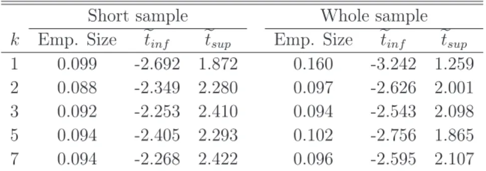
There still remains one potential problem in our regressions, as the empirical size of the Newey–West t–statistic ought to be distorted. Therefore, in Table 1.3 we report (i) the empirical size of the t–statistic should it be used in the conventional way (using 1.96 as the threshold), and (ii) the correct thresholds that guarantee a 5% two–sided confidence level in our sample.

— Table 1.3 about here —

Table 1.3 clearly shows that the size of the Newey–West t–statistics are distorted. For example, applying the standard threshold values associated to the two–sided t– statistics at the conventional 5% significance level would actually yield a 10% size in both samples. The empirical size even rises to 16% in the whole sample for the

1.1. Empirical Evidence 41

shortest horizon. In other words, this would lead the econometrician to reject the absence of predictability too often. But the problem is actually more pronounced as can be seen from columns 3, 4, 6 and 7 of Table 1.3. Beside the distortion of the size of the test, an additional problem emerges: the distribution are skewed, which implies that the tests are not symmetric. This is also illustrated in Figures 1.3 and 1.4 (see Appendix B) which report the cdf of the Student distribution and the distribution obtained from our Monte-carlo experiments. Both figures show that the distributions are distorted and that this distortion is the largest at short horizons. Therefore, when running regressions on the data, we will take care of these two phenomena.

We ran the predictability regressions on actual data correcting for the aforemen-tioned problems. The results are reported in Table 1.4.

— Table 1.4 about here —

Panels (a) and (b) report the predictability coefficients obtained from the esti-mation of equation (1.1.1). The second line of each panel reports the t–statistic, tk,

associated to the null of the absence of predictability together with the empirical size of the test. Then the fourth line gives the modified t–statistics, ck, proposed by

Valkanov [2003] which correct for the size of the sample (ck = tk/

√

T ) and the as-sociated empirical size. The empirical size used for each experiments were obtained from 100,000 Monte Carlo simulations and therefore corrects for the size distorsion problem. Finally, the last line reports information on the overall fit of the regression. The estimation results suggest that excess returns are negatively related to the price–dividend ratio whatever the horizon and whatever the sample. Moreover, the larger the horizon, the larger the magnitude of this relationship is. For instance, when the lagged price–dividend ratio is used to predict excess returns, the coefficient is -0.362 in the short sample, while the coefficient is multiplied by around 4 and

rises to -1.414 when 7 lags are considered. In other words, the price–dividend ratio accounts for greater volatility at longer horizons. A second worth noting fact is that the foreseeability of the price–dividend ratio is increasing with horizon as the R2 _{of the regression increases with the lag horizon. For instance, the one year}

predictability regression indicates that the price–dividend ratio accounts for 22% of the overall volatility of the excess return in the short run. This share rises to 68% at the 7 years horizon. It should however be noticed that the significance of this relationship fundamentally depends on the sample we focus on. Over the short sample, predictability can never be rejected at any conventional significance level, whether we consider the standard t–statistics or the corrected statistics. The empirical size of the test is essentially zero whatever the horizon for both tests. The evidence in favor of predictability is milder when we extend the sample up to 2001. For instance, the empirical size of the null of no predictability is about 17% over the short horizon, and rises to 30% at the 5 years horizon. This lack of significance is witnessed by the measure of fit of the regression which amounts to 29% over the longer run horizon. This finding is related to the fact that while excess return remained stable over the whole sample, the price–dividend ratio started to raise in the latest part of the sample, therefore dampening its predictive power. Taken together, these findings suggest that the potential lack of predictability of the price dividend ratio essentially reflects some sub–sample issues rather than a deep econometric problem. The late nineties were marked by a particular phase of the evolution of stock markets which seems to be related to the upsurge of the information technologies, which may have created a transition phase weakening the predictability of stock returns (see Hobijn and Jovanovic [2001] for an analysis of this issue). This issue is far beyond the scope of this paper. Nevertheless, the data suggest that the price dividend ratio offered a pretty good predictor of stock returns at least in the pre–information technology revolution.

1.2. Catching–up with the Joneses 43

1.2

Catching–up with the Joneses

In this section, we develop a consumption based asset pricing model in which pref-erences exhibit a “Catching up with the Joneses” phenomenon. We provide the closed–form solution for the price–dividend ratio and conditions that guarantee the existence of a stationary bounded equilibrium.

1.2.1

The model

We consider a pure exchange economy à la Lucas [1978]. The economy is populated by a single infinitely–lived representative agent. The agent has preferences over consumption, represented by the following intertemporal expected utility function

Et ∞ X s=0 βs_u t+s (1.2.4)

where β > 0 is a constant discount factor, and ut denotes the instantaneous utility

function, that will be defined later. Expectations are conditional on information available at the beginning of period t.

The agent enters period t with a number of shares, St —measured in terms of

consumption goods— carried over the previous period as a means to transfer wealth intertemporally. Each share is valuated at price Pt. At the beginning of the period,

she receives dividends, DtSt where Dt is the dividend per share. These revenues

are then used to purchase consumption goods, ct, and new shares, St+1, at price Pt.

The budget constraint therefore writes

PtSt+1+ Ct6 (Pt+ Dt)St (1.2.5)

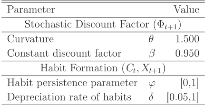
Following Abel [1990,1999], we assume that the instantaneous utility function, ut, takes the form

ut≡ u(Ct, Vt) =      (Ct/Vt)1−θ−1 1−θ if θ ∈ R+\{1} log(Ct) − log(Vt) if θ = 1 (1.2.6)

where θ measures the degree of relative risk aversion and Vt denotes the habit level.

We assume Vtis a function of lagged aggregate7 consumption, Ct−1, and is

there-fore external to the agent. This assumption amounts to assume that preferences are characterized by a “Catching up with the Joneses” phenomenon.8 _{More precisely,}

we assume that9

Vt = C ϕ

t−1 (1.2.7)

where ϕ > 0 rules the sensitivity of household’s preferences to past aggregate con-sumption, Ct−1, and therefore measures the degree of “Catching up with the Joneses”.

It is worth noting that habit persistence is specified in terms of the ratio of current consumption to a function of lagged consumption. We hereby follow Abel [1990] and depart from a strand of the literature which follows Campbell and Cochrane [1999] and specifies habit persistence in terms of the difference between current and a reference level. This particular feature of the model will enable us to obtain a closed form solution to the asset pricing problem while keeping the main properties of habit persistence. Indeed, as shown by Burnside [1998], one of the keys to a closed form solution is that the marginal rate of substitution between consumption at two dates is an exponential function of the growth rate of consumption between these two dates. This is indeed the case with this particular form of catching up. An-other implication of this specification is that, just alike the standard CRRA utility function, the individual risk aversion remains time–invariant and is unambiguously

7_{Appendix A provides a closed form solution to the proposed model under the assumption of}

internal habit formation. More precisely, we assume that the reference level is function of the individual’s own past consumption:

Vt= Ct−1ϕ

8_{Note that had V}

tbeen a function of current aggregate consumption, we would have recovered

Galí’s [1989] “Keeping up with the Jones”. In such a case the model admits that same analytical solution as in Burnside [1998].

9_{Note that this specification of the preference parameter can be understood as a particular case}

of Abel [1990] specification which is, in our notations, given by Vt= [Ct−1D C

1−D

t−1 ]γ with 0 6 D 6 1

1.2. Catching–up with the Joneses 45

given by θ.

Another attractive feature of this specification is that it nests several standard specifications. For instance, setting θ = 1 leads to the standard time separable case, as in this case the instantaneous utility function reduces to log(Ct) − ϕ log(Ct−1).

As aggregate consumption, Ct−1, is not internalized by the agents when taking

their consumption decisions, the (maximized) utility function actually reduces to Et

P_∞

s=0βslog(Ct+s). The intertemporal utility function is time separable and the

solution for the price–dividend ratio is given by Pt/Dt= β/(1 − β).

Setting ϕ = 0, we recover a standard time separable CRRA utility function of the form Et

P_∞

s=0βs(Ct+s1−θ− 1)/(1 − θ). In such a case, Burnside [1998] showed that

as long as dividend growth is log–normally distributed, the model admits a closed form solution.10

Setting ϕ = 1 we retrieve Abel’s [1990] relative consumption case (case B in Table 1, p.41) when shocks to endowments are iid. In this case, the household values increases in her individual consumption vis à vis lagged aggregate consumption. In equilibrium, Ct−1= Ct−1 and it turns out that utility is a function of consumption

growth.

At this stage, no further restriction will be placed on either β, θ or ϕ.

The household determines her contingent consumption {Ct}∞t=0 and contingent

asset holdings {St+1}∞t=0plans by maximizing (1.2.4) subject to the budget constraint

(1.2.5), taking exogenous shocks distribution as given, and (1.2.6) and (1.2.7) given. Agents’ consumption decisions are then governed by the following Euler equation

PtCt−θC ϕ(θ−1) t−1 = βEt h (Pt+1+ Dt+1)Ct+1−θC ϕ(θ−1) t i (1.2.8) which may be rewritten as

Pt Dt = Et ·µ 1 + Pt+1 Dt+1 ¶ × Wt+1× Φt+1 ¸ × Ct (1.2.9)

10_{Note that this result extends to more general distribution. See for example Bidarkota and}

where Wt+1 ≡ Dt+1/Dtcaptures the wealth effect of dividend, Φt+1 ≡ β[(Ct+1/Ct)−θ]

is the standard stochastic discount factor arising in the time separable model. This Euler equation has an additional stochastic factor Ct ≡

¡

Ct/Ct−1

¢_ϕ(θ−1)

which mea-sures the effect of “catching up with the Joneses”. These two latter effects capture the intertemporal substitution motives in consumption decisions. Note that Ct is

known with certainty in period t as it only depends on current and past aggregate consumption. This new component distorts the standard intertemporal consump-tion decisions arising in a standard time separable model. Note that our specificaconsump-tion of the utility function implies that ϕ essentially governs the size of the catching up effect, while risk aversion, θ, governs its direction. For instance, when risk aversion is large enough — θ > 1 — catching–up exerts a positive effect on the time sep-arable intertemporal rate of substitution. Hence, in this case, for a given rate of consumption growth, catching up reduces the expected return.

Since we assumed the economy is populated by a single representative agent, we have St = 1 and Ct = Ct= Dt in equilibrium. Hence, both the stochastic discount

factor in the time separable model and the “ ‘catching up with the Joneses” term are functions of dividend growth Dt+1/Dt

Φt+1 ≡ β[(Dt+1/Dt)−θ] and Ct ≡ (Dt/Dt−1)ϕ(θ−1)

Any persistent increase in future dividends, Dt+1, leads to two main effects in the

standard time separable model. First, a standard wealth effect, stemming from the increase in wealth it triggers (Wt+1), leads the household to consume more

and purchase more assets. This puts upward pressure on asset prices. Second, there is an effect on the stochastic discount factor (Φt+1). Larger future dividends

lead to greater future consumption and therefore lower future marginal utility of consumption. The household is willing to transfer t + 1 consumption toward period t, which can be achieved by selling shares therefore putting downward pressure on prices. When θ > 1, the latter effect dominates and prices are a decreasing

1.2. Catching–up with the Joneses 47

function of dividend. In the “catching up” model, a third effect, stemming from habit persistence (Ct), comes into play. Habit standards limit the willingness of the

household to transfer consumption intertemporally. Indeed, when the household brings future consumption back to period t, she hereby raises the consumption standards for the next period. This raises future marginal utility of consumption and therefore plays against the stochastic discount factor effect. Henceforth, this limits the decrease in asset prices and can even reverse the effect when ϕ is large enough.

Defining the price–dividend ratio as vt = Pt/Dt, it is convenient to rewrite the

Euler equation evaluated at the equilibrium as vt= βEt " (1 + vt+1) µ Dt+1 Dt ¶_1−θµ Dt Dt−1 ¶_ϕ(θ−1)# (1.2.10)

1.2.2

Solution and existence

In this section, we provide a closed form solution for the price–dividend ratio and give conditions that guarantee the existence of a stationary bounded equilibrium.

Note that up to now, no restrictions have been placed on the stochastic process governing dividends. Most of the literature attempting to obtain an analytical solu-tion to the problem assumes that the rate of growth of dividends is an iid Gaussian process (see Abel [1990,1999] among others).11 _{We depart from the iid case and}

follow Burnside [1998]. We assume that dividends grow at rate γt ≡ log(Dt/Dt−1),

and that γt follows an AR(1) process of the form

γt= ργt−1+ (1 − ρ)γ + εt (1.2.11)

where εt; N(0, σ2) and |ρ| < 1. In the AR(1) case, the Euler equation rewrites

vt = βEt[(1 + vt+1) exp ((1 − θ)γt+1− ϕ(1 − θ)γt)] (1.2.12)

11_{There also exist a whole strand of the literature introducing Markov switching processes in}

CCAPM models. See Cecchetti, Lam and Mark [2000] and Brandt, Zeng and Zhang [2004] among others.