The trade-o¤ between work and informal care in Europe
Roméo Fontaine*
(LEDa-LEGOS, Université Paris-Dauphine)
March 31, 2011
Abstract
This paper focus on the trade-o¤ between work and informal care among individuals aged 50 to 65. We …rst outlines the standard microeconomic model used to study how individuals allocate their time between labour, parental care and leisure. From the two …rst-order conditions of the standard model, we jointly estimate the time devoted to work and care through a bi-tobit model allowing to take into account both the simultaneity of the decisions and the censure which characterizes each variable. The model is estimated using data from SHARE, a European multidisciplinary database of micro data on health, socio-economic status and family network. Estimation results do not appear consistent with the standard microeconomic framework and lead us to reformulate the microeconomic model in order to take into account a potential positive e¤ect of the worker status on the propensity to provide care The reformulation proposed is empirically validated by the the estimation of a double selection model. Our main …nding con…rms results of qualitative survey and suggests that the e¤ect of paid work on time devoted to care may be decompose into (i) a discret positif e¤ect, the labour market participation a¤ecting positively the propensity to provide care, and (ii) a continuous negative e¤ect, each worked hour reducing time devoted to parental care.
Acknowledgements : I would like to warmly thank Agnès Gramain and Jérôme Wittwer, my PhD advisors, who helped and guided me throughout this work. I am grateful to Marie-Eve Joël, Steven Stern and François-Charles Wol¤ for their valuable comments and suggestions on previous versions of this paper.
*Correspondence to : Université Paris-Dauphine, LEDa-LEGOS, Place du Maréchal de Lattre de Tassigny 75775 Paris Cedex 16, France. E-mail : [email protected]
1 Introduction
Population ageing is considered in Europe as a major challenge in the coming decades, especially because of the sustainability question of public pensions systems. To contain the dependency ratio, the Stockholm European Council (2001) has set a target for Member States to raise the employment rate to a European average of 67%, setting speci…c objectives for the senior population. According to the Stockholm European Council conclusions, “it has agreed to set an EU target for increasing the average EU employment rate among older women and men (55-64) to 50 % by 2010”1. This
target of 50% was subsequently renewed by the Community Lisbon Program (2005).
In parallel, the growing proportion of elderly in the population is likely to increase the demand for long-term care. To allow the frail elderly to live in the community without excessively increasing public long-term care expenditures, most of the EU members encourage, more or less explicitly, family members to provide care for elderly people.
Considering that senior play a major role in caring for dependent elderly people, it is appropriate to ask whether a policy aimed at extending the work lives of seniors is compatible with a policy aimed at supporting informal care for elderly people. Won’t informal care decrease if the senior employment rate rises ? Or, looking at it from the opposite side, won’t shifting the burden of care for elderly people to families hamper growth in senior employment ?
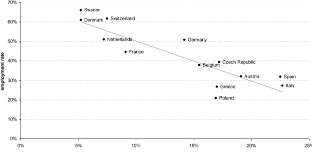
Using data from the second wave of the Survey of Health, Ageing and Retirement in Europe (SHARE, 2006-2007)2, …gure 1 illustrates at the national level the relationship between the
em-ployment rate for women aged 50 to 65 with one living parent3, with the proportion of “intensive” caregivers, de…ned as those who devote to parental care more than one hour a day or who co-reside with their parent. A decreasing relationship appears between the labour force participation and the provision of informal care. At one end, there are Northern European countries and Switzerland, which present a high employment rate and a low proportion of intensive caregivers. At the other end are the countries of Southeast and Eastern European characterized by a low employment rate
1In 2001, the European employment rate of this population was 37.7% (Eurostat). 2See section 3 for a description of the data.
3We focus in this chapter on caregiving provided by children to their parent living without a spouse. Children caregiving behaviour greatly depends on the presence or absence of a spouse caregiver (see chapter 1).
and a high proportion of intensive caregivers. Continental European countries lie somewhere in between.
Figure 2 highlights a similar negative correlation at the individual level : the women labour force participation decreases according to the intensity of care provided for a non-coresiding elderly parent. It appears however that women who provide less than an hour a day of care are more frequently employed than no caregivers. This result suggests that the relationship between work and care is not only based on a pure substitution e¤ect between the two activities.
The aim of this paper is to highlight the individual interaction process between working and caregiving behaviour among the senior population. We …rst present the standard individual time allocation model between paid work, leisure and parental care. The model produces testable im-plications. In particular, working time and caregiving time appears as two competing activities : every exogenous shocks a¤ecting positively one activity leads to a reducation of time devoted to the other activity. In order to test the implications of this model, we estimate a bi-tobit model allowing to take into account the simultaneously of the care and work decision and the censure which characterized each variable. Estimation results do not appear consistent with the standard microeconomic framework and lead us to reformulate it in order to take into account a potential positive e¤ect of worker status on the propensity to provide parental care. The estimation of a double selection model provides results consistent with the reformulated microeconomic model. Indeed, our main …nding suggests that the e¤ect of paid work on time devoted to care may be decompose into a discret positif e¤ect, the labour market participation a¤ecting positively the pro-pensity to provide care, and a continuous negative e¤ect, each worked hour reducing time devoted to parental care.
The rest of this article is organized as follows. Section 2 reviews the previous literature. Section 3 outlines the data used in the analysis. Section 4 presents a simple microeconomic model of the trade-o¤ between labour and care. Section 5 empirically tests the implication of the model. Section 6 outlines a reformulation of the standard microeconomic framework. Section 7 provides an empirical validation of this new microeconomic framework. Finally, section 8 concludes.
Figure 1. Employment rate and proportion of « intensive » caregivers by country (women only) Austria Germany Netherlands Italy France Denmark Greece BelgiumCzech Republic
Poland Sweden Spain Switzerland 0% 10% 20% 30% 40% 50% 60% 70% 0% 5% 10% 15% 20% 25%
proportion of "intensive" caregiver
em p lo ym en t rate
Population : Women aged 50 to 65 and having only one living parent. Source : Eurostat and SHARE, wave 2 (2006-2007)
Figure 2. Employment rate of women according to the intensity of care
0% 10% 20% 30% 40% 50% 60% 70% nocaregiver ] 0 ; 1 ] ] 1 ; 2 ] ] 2 ; 4 ] ] 4 ; 8 ] ] 8 ; +]
num ber of hours of care per day
em p lo ym en t rat e
Population : Women aged 50 to 65 and having only one living parent (women co-residing with their elderly parent are excluded because of lack of information on their caregiving behaviour) Source : SHARE, wave 2 (2006-2007)
2 Previous literature
Since the mid-80s, several empirical studies have analysed the relationship between labour and caregiving behaviour.
The literature is very heterogeneous with regards to the studied population and the measure of the outcomes related to labour supply and care provision. Most studies investigate the interaction between care provision and labour supply on particular samples, restricted the analysis to informal caregivers (Muurinen, 1986 ; Stone et al., 1987 ; Stone and Short,1990 ; Boaz and Muller, 1992), married daughters (Wolf and Soldo, 1994), daughters (Ettner, 1995 ; Pezzin and Schone, 1995 ; Kolodinsky and Shirey, 2000 ; Crespo, 2006), women (Mac Lanahan and Manson, 1990 ; Pavalko and Artis, 1997 ; Carmichael and Charles, 1998 ; Spiess and Schneider, 2002 ; Berecki-Gisolf et al., 2008 ; Casado-Marin et al., 2007), child (Börsch-Supan et al., 1992 ; Stern, 1995 ; Ettner 1996 ; Johnson and Lo Sasso, 2000, Bolin et al., 2007), while others only restricted the sample according to an age criteria, in order to select a population of working-age (Carmichael and Charles, 2003a ; Carmichael and Charles, 2003b ; Heitmueller, 2007 ; Huetmueller and Inglis, 2007, Carmichael and Charles, 2010). Note also that the care receiver di¤ers among the studies. Some studies only consider the care provide to parents, whereas others restricted to single parent or extend the potential care receiver to step-parents, parents in law, spouses, children or non-members of the family.
With regard to the outcome measure, several studies consider binary outcomes (provide care or not, participate to the labour market or not) while others used ordinal outcomes (do not provide care/provide non-intensive care/provide intensive care, do not participate to the labour market/work part-time/work full time), non-ordinal outcomes (do not provide care/provide care outside the household/provide care to a co-resident) or censored outcomes (the time devoted to care or time spent working).
However, with regards to our study, the two main cleavages in the literature concern the cau-sality direction empirically investigated and the way to deal with the endogeneity issues. Existing literature generally focuses on one pathway of causation4.
4Pezzin and Schone (1999) and Borsch-Supan et al. (1992) estimate structural models allowing to identify how the two endogenous outcomes related to work and care react to changes in exogenous variables. These models do
* Causality direction : from care provision to labour supply
A large majority of studies focuses on the e¤ect of the care provision on the labour supply. From this point of view the care provision is seen as a determinant of the labour supply.
Muurinen (1986), using a US sample of primary caregivers of terminally-ill patients in a hospice setting, …nd that the care provision leads to either withdrawal from the labour market or reduced hours of work.
Stone et al. (1987) and Stone and Short (1990) use the US Informal Caregivers Survey (ICS), a supplement to the 1982 National Long Term Care Survey (NLTC) and …nd that the care activity leads to work accommodations, such as rearrangements of work schedule, reductions in work hours, or taking unpaid leave. These three studies however used sample containing only caregivers. This restriction does not allow to generalize the results to the overall population. Results obtained with more representative samples leads however to similar conclusions.
Using data from the 1987-1988 National Survey of Families and Household (NFSFH), Mac Lanahan and Manson (1990) …nd that the care provision signi…cantly reduces the probability to work and the conditional hours worked per week.
Kolodinsky and Shirey (2000), using the Panel Study of Income Dynamics (PSID), study the e¤ect of co-residence with an elder parent on the labour supply. They …nd that the presence and the characteristics of the parents negatively impact the labour market participation and the time spent working.
In Europe, the …rst empirical studies have been conducted in UK. Using a sample of women aged 21 to 59 from the 1985 General Household Survey (GHS), Carmichael and Charles (1998) show that the impact of the care provision on the labour supply depends on the intensity of care. They …nd that providing less than 20 hours per week of care increase the probability of employment whereas providing more than 20 hours per week of care decreases the labour market participation. Using the 1990 General Household Survey, the same authors …nd that the negative e¤ect of caregiving beyond a certain threshold would be lower for men than for women and that the
not allow to directly identify the causality between the two variables. However, the estimation of the structural parameters suggests in both cases that the trade-o¤s between labor supply and parental caregiving decisions is relatively modest.
negative e¤ect on employment is greater for those caring for someone living in the same household (Carmichael and Charles, 2003a ; Carmichael and Charles, 2003b).
The main limitation of these empirical studies is the exogeneity assumption of the caregiving behaviour. This assumption is very questionable. Indeed, the labour behaviour may act as a de-terminant of the care provision. For instance, not working can favour the informal care provision since non-workers generally face lower opportunity costs than workers. This reversal causality may then bias the estimation of the e¤ect of the care provision on the labour supply.
To take into account the potential simultaneity of decisions regarding employment and care, most studies use an instrumental variable approach. The model generally includes two equations : a reduced instrumental equation of the care provision and a structural equation of the labour supply including the instrumented care provision as regressor. The model is then estimated either in two-step or simultaneously by maximum likelihood.
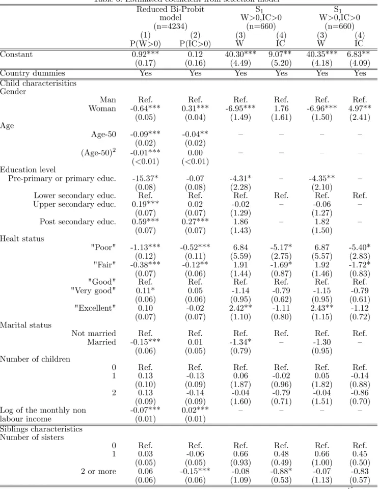
Using data from the National Survey of Families and Households (NSFH), Wolf and Soldo (1994) estimated a two step model. In the …rst step, they simultaneously estimated a reduced form of the probability to provide parental care and to be employed. In the second step, they estimate the e¤ect of being caregiver on the hours of work, conditionally on the labour market participation. They use a double-selection framework by adding as regressors two correction terms computed from the …rst step. The …rst have to be seen as a standard selection term allowing to correct the selection of the workers whereas the second one have to be seen as an augmented regressor allowing to control for the correlation between the care provision and the residual of the work hours equation. They …nd that the provision of parental care among married daughters does not signi…cantly reduce their propensities to be employed or their conditional hours of work.
Ettner (1995, 1996) adopt a similar empirical strategy but uses a two part model instead of a selection model. From the 1986-1988 panels of the Survey of Income and Program Participation (SIPP), results suggest that coresidence with a disabled parent signi…cantly reduces hours worked among females aged 35 to 64, due primarily to withdrawal from the labour market. However, she …nds no signi…cant reduction of work hours due to nonhousehold member caregiving (Ettner, 1995). Ettner (1996), using the same data than Wolf and Soldo (1994) shows that the magnitude of the caregiving impact on the labour supply is larger for women than for men and for coresidence
than for non-coresidential care. However, the e¤ect was signi…cant only for women providing care to parents residing outside the household.
Johnson and Lo Sasso (2000) simultaneously estimate a structural equation of the annual hours of paid work (taking into account the censoring of the variable) and a reduced equation of the care provision, using US panel data from the Health and Retirement Study (HRS). Restricting the sample to men and women aged 53 to 65 and having at least one living parent, they identify a signi…cant negative e¤ect of providing care to parents on the labour supply for both women and men.
Crespo (2006) estimates a bivariate probit model on a sample of women aged 50 to 60 with at least one living parent from the …rst wave of the Survey of Health, Ageing and Retirement in Europe (SHARE). Results suggest that providing “intensive” informal care to parents negatively impacts the labour market participation.
Heitmueller (2007), from the British Household Panel Study, adopts a standard IV approach and …nd that providing care to a coresident reduces the propensity to work whereas no signi…cant e¤ect is found for extra-household care provision.
Bolin et al. (2007) adopts the same empirical strategy, using data from the …rst wave of SHARE. Results suggest than the care provision negatively impact the participation to the labour market and the hours of work among workers.
Casado-Marin et al. (2008) exploit data from the European Community Household Panel (1994-2001). They use treatment evaluation techniques (matching method and di¤erences in di¤erences) to estimate the e¤ects of caregiving on the labour market participation for women aged between 30 to 60. Results suggest that among women who were working before becoming a caregiver, there is no signi…cant reduction in the probability of being employed. However, for those who were not working prior to becoming a caregiver, there is a signi…cant decrease in the chances of entering employment.
To summarize, a large majority of studies provide evidence of a sign…cant negative e¤ect of caregiving on the labour supply, while others generally identify a negative but no signi…cant ef-fect. Taking into account the endogeneity of the care provision does not change this main result.
However, all the previous mentioned studies using an IV approach show that not accommodating for endogeneity of the care provision in the labour outcome equation overestimate the real impact of an exogenous variation of caregiving (see Wolf and Soldo, 1994 ; Ettner, 1995 ; Ettner, 1996 ; Jonhson et Lo Sasso, 2000 ; Crespo, 2006 ; Heitmueller, 2007 ; Bolin et al., 2007). Speci…cally, all these studies provide evidence of a positive correlation between the care variable and the residual of the labour outcome equation. This positive correlation, interpreted in terms of simultaneity bias, tends to suggest a positive reversal causality, that is a positive e¤ect of the labour supply on the propensity to provide care. As noted for instance by Ettner (1995) or Heitmueller (2007), this empirical result appears inconsistent with the standard conceptual framework which suggests the existence of a negative reversal causality and thus a decline, in absolute terms, of the impact of the care variable when endogeneity is controlled.
*Causality direction : from labour supply to care provision
To the best of our knowledge, very few studies aim to identify how an exogenous shock on the labour supply impacts the provision of care.
Using personal interview data on 460 persons with noncoresidential parent, Spitze and Logan (1991) examine the impact of work hours on several parent care outcomes (frequency of interactions, patterns of help and attitude toward the relashionship. They use OLS estimation and do not …nd signi…cant e¤ect of employment on caregiving or interactions with the parent.
Börsch-Supan et al. (1992), who use data from Massachusetts (1986 HRCA Elderly Survey and 1986 HRC-NBER Child Survey), estimate a Tobit model and identify a signi…cant positive e¤ect of employment (treated as exogenous) on time spent with parents5.
Stern (1995) adopts an IV approach with panel data using two waves (1982 and 1984) of the NLTC Survey. The author estimates in the second year how the children’s probability to be the primary caregiver is a¤ected by their work status. By restricting the sample to parents receiving no care in the …rst year he uses as instrument of the labour force status of each child for the second year the labour force status of the …rst year. After controlling for endogeneity, results suggest that work status does not signi…cantly a¤ect the care provision.
5This positive e¤ect appears consistent with the positive correlation between the care provision (as regressor) and the residual of the labour supply outcome.
Carmichael and Charles (2010) use a similar approach from 15 waves (1991-2005) of the British Household Panel Survey (BHPS). They …nd no signi…cant e¤ect of working less than 20 hours per week and a negative e¤ect of working more than 20 hours a week (in t) on the probability to become caregiver (in t+1). Moreover, among those employed, they do not …nd a signi…cant e¤ect of working time (in t) on the probability to become caregiver (in t+1).
To summarize, this pathway of causation appears less clear than the opposite one. Only Car-michael and Charles (2010) …nd a negative e¤ect of labour supply on the care provision (and only for those who work more than 20 hours per week). Others studies …nd a no signi…cant or a positive e¤ect.
* When both causality directions are simultaneously investigated
Finally, Boaz and Muller (1992), Pavalko and Artis (1997), Spiess and Schneider (2002) and Berecki-Gisolf (2008) jointly estimate the two opposite pathway of causation. Overall, these studies con…rm the main message of the literature : an exogenous increase of the care provision a¤ects negatively and generally signi…cantly the labour supply whereas an exogenous variation of the labour supply have an unclear but generally not signi…cant e¤ect on the care provision.
Boaz and Muller (1992) use a sample from the National Informal Caregivers Survey (NICS) which only include active caregivers. They use a two-step estimation. They …rst regress the weekly hours of unpaid help and the work status, measured with an ordinal variable with three modalities (no work, part-time work, full-time work) on all the exogenous variables of the model in order to obtain predicted values uncorrelated with the model’s error terms. These predicted values are used to replace the endogenous RHS variables in the second stage equations, which are the structural equations of the model. Results suggest that conditionally on being caregiver, time devoted to care signi…cantly reduces the probability to work full-time but not the probability to work part-time. Symmetrically, working full-time signi…cantly reduces the care provision whereas working part-time does not a¤ect time devoted to care.
Pavalko and Artis (1997), who use panel data from the National Longitudinal Survey of Mature Women, …nd that women aged 50 to 64 who start providing care signi…cantly reduce hours of paid employment. On the contrary, the work status does not signi…cantly impact the propensity to start providing care.
Berecki-Gisolf et al. (2008) and Spiess and Schneider (2002) obtain similar results from the Australian Longitudinal Study on Women’s Health (ALSWH) and the European Community Hou-sehold Panel (SCHP). Spiess and Scheinder (2002) …nd however that being employed reduced the probability to provide care more than 14 hours per week.
3 Data
For our analysis, we use the second wave (2006-2007) of the Survey of Health, Ageing and Retirement in Europe (SHARE). SHARE follows the design of the US Health and Retirement Study (HRS) and the English Longitudinal Study of Ageing (ELSA). It is a multidisciplinary database of micro data on health, socio-economic status and social and family networks of more than 30 000 individuals aged 50 or over.
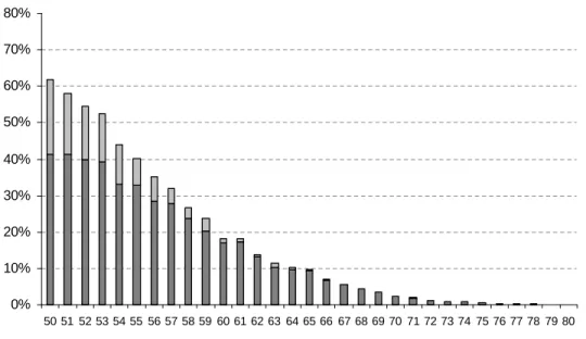
For the purpose of this study, we restricted the sample to people aged 50 to 65, not only because, over 65, the probability to work is close to zero, but also because the proportion of those having at least one living parent is very low (…gure 3).
We focus the analysis on care provided for elderly parent. Alternatively, we could have focused on care provided by individuals to their dependent spouse but adverse e¤ects on labour behaviour are less expected given that it generally concerns elder caregivers who are already retired. As previously mentioned, we also restricted the sample to respondents having a single living parent. Moreover, because of a lack of information on intra-household caregiving we had to exclude children living with their elderly parent. The …nal sample includes 4234 observations.
Figure 3. Proportion by age of individuals having at least one living parent 0% 10% 20% 30% 40% 50% 60% 70% 80% 50 51 52 53 54 55 56 57 58 59 60 61 62 63 64 65 66 67 68 69 70 71 72 73 74 75 76 77 78 79 80 age
one living parent two living parents
In order to study the interaction between care and paid work, we use two variables : the number of hours worked per week (W ) and the number of hours per week devoted to parental care (IC). Time devoted to care combines three activities : personal care, practical household help and help with paperwork. One can assume that the articulation between care and labour supply di¤ers according to the kind of care. For instance, it can be easier to articulate help with paperwork and work because this kind of care can be provided remotely. On the contrary, personal care can require an personal investment of time and emotional more binding. However, the data does not allow to distinguish time devoted to each kind of care. We then consider global caregiving time without distinguish the kind of care. Note also that our de…nition of caregiving does not take into account moral support provided by the the child to his/her elderly parent. Concerning working time, we adopt a broad de…nition. We use here the information on the number of hours a week the child usually work, regardless of his/her basic contracted hours. Alternatively, it could be possible to use the information on contracted hours but in this case, we should exclude from the analysis self-employed for whom the information on contracted hours is not available. Our choice may potentially a¤ects the results because extra-contracted working hours are probably more related to caregiving behaviour than contracted hours.
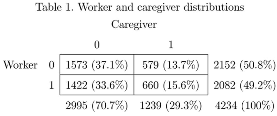
sample are employed and 29% provide care for their elderly parent (table 1).
Table 1. Worker and caregiver distributions Caregiver
0 1
Worker 0 1573 (37.1%) 579 (13.7%) 2152 (50.8%) 1 1422 (33.6%) 660 (15.6%) 2082 (49.2%) 2995 (70.7%) 1239 (29.3%) 4234 (100%)
The optimal time allocation is assumed to depend on three groups of variables. The …rst corresponds to the individual socio-demographic characteristics : age, education level, marital status, number of children, health status and the non labour income. We do not use the wages as explanatory variable even if the information is available for workers. As emphasized by Ettner (1995), the imputation of wage rates for non workers involves identi…cation issues because the variables that in‡uence the potential wage rate are likely to directly impact the choice of work hours. Following Ettner (1995) and Dimova & Wol¤ (2010), we therefore include determinants of wage rate in the working time equation, such as age or education level, rather than the wage itself. The second group of variables corresponds to the parent’s characteristics. In our estimations, we control for the parent’s gender, age and health status but also for the geographical proximity between the child and the parent. To measure the parental health status we only have a variable indicating how the child evaluate the general health status of his/her parent. In particular, no information is available on the parent’s incapacity level, even though it may be partially captured by the parent’s age variable. Moreover, we do not know if the parent lives in the community or in a nursing home and if he or she receives formal care. This lack of information may lead to a negative coe¢ cient correlation between the residuals of the two equations if, for instance, professional care (in institution or in the community) encourages the child to increase his/her working time (to …nance the professional care) and reduces the caregiving time.
Finally, the third group of explanatory variables corresponds to the siblings’ characteristics. Our estimations include as explanatory variables the number of brothers, the number or daughters and the birth rank of the respondent. We distinguish the number of siblings according to their gender in order to take into account that daughters are more likely to provide care than sons.
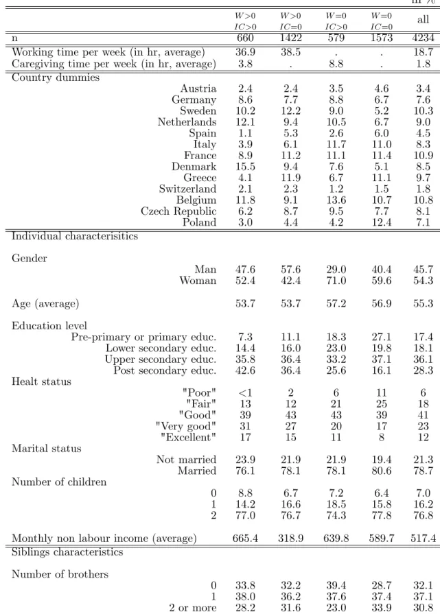
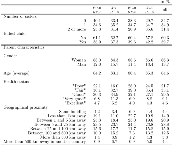
Table 2 reports the distribution of each variables used among sub-samples (according to the working and caregiving behavior) and for the overall sample.
Table 2. Distribution of the variables used
in % W >0 IC>0 W >0 IC=0 W =0 IC>0 W =0 IC=0 all n 660 1422 579 1573 4234
Working time per week (in hr, average) 36.9 38.5 . . 18.7
Caregiving time per week (in hr, average) 3.8 . 8.8 . 1.8
Country dummies Austria 2.4 2.4 3.5 4.6 3.4 Germany 8.6 7.7 8.8 6.7 7.6 Sweden 10.2 12.2 9.0 5.2 10.3 Netherlands 12.1 9.4 10.5 6.7 9.0 Spain 1.1 5.3 2.6 6.0 4.5 Italy 3.9 6.1 11.7 11.0 8.3 France 8.9 11.2 11.1 11.4 10.9 Denmark 15.5 9.4 7.6 5.1 8.5 Greece 4.1 11.9 6.7 11.1 9.7 Switzerland 2.1 2.3 1.2 1.5 1.8 Belgium 11.8 9.1 13.6 10.7 10.8 Czech Republic 6.2 8.7 9.5 7.7 8.1 Poland 3.0 4.4 4.2 12.4 7.1 Individual characterisitics Gender Man 47.6 57.6 29.0 40.4 45.7 Woman 52.4 42.4 71.0 59.6 54.3 Age (average) 53.7 53.7 57.2 56.9 55.3 Education level
Pre-primary or primary educ. 7.3 11.1 18.3 27.1 17.4
Lower secondary educ. 14.4 16.0 23.0 19.8 18.1
Upper secondary educ. 35.8 36.4 33.2 37.1 36.1
Post secondary educ. 42.6 36.4 25.6 16.1 28.3
Healt status "Poor" <1 2 6 11 6 "Fair" 13 12 21 25 18 "Good" 39 43 43 39 41 "Very good" 31 27 20 17 23 "Excellent" 17 15 11 8 12 Marital status Not married 23.9 21.9 21.9 19.4 21.3 Married 76.1 78.1 78.1 80.6 78.7 Number of children 0 8.8 6.7 7.2 6.4 7.0 1 14.2 16.6 18.5 15.8 16.2 2 77.0 76.7 74.3 77.8 76.8
Monthly non labour income (average) 665.4 318.9 639.8 589.7 517.4
Siblings characteristics Number of brothers 0 33.8 32.2 39.4 28.7 32.1 1 38.0 36.2 37.6 37.4 37.1 2 or more 28.2 31.6 23.0 33.9 30.8 (continue...)
Table 2. Continue... in % W >0 IC>0 W >0 IC=0 W =0 IC>0 W =0 IC=0 all Number of sisters 0 40.1 33.4 38.3 29.7 34.7 1 34.6 35.2 34.7 34.7 34.9 2 or more 25.3 31.4 26.9 35.6 31.4 Eldest child No 61.1 62.7 60.4 57.8 60.3 Yes 38.9 37.3 39.6 42.2 39.7 Parent characteristics Gender Woman 88.0 84.3 88.6 86.6 86.3 Man 12.0 15.7 11.4 13.4 13.7 Age (average) 84.2 83.1 86.4 85.3 84.6 Health status "Poor" 22.1 16.0 28.0 24.5 21.7 "Fair" 36.1 32.7 39.0 35.4 35.1 "Good" 30.3 34.9 22.1 27.1 29.5 "Very good" 6.8 11.3 6.9 8.8 9.1 "Excellent" 4.7 5.2 4.0 4.3 4.6 Geographical proximity Same building 4.2 3.4 6.9 4.4 4.4
Less than 1km away 19.1 11.0 22.7 19.9 14.9
Between 1 and 5 km away 25.3 18.4 25.0 19.6 20.9
Between 5 and 25 km away 23.5 23.7 24.4 23.8 28.8
Between 25 and 100 km away 15.6 17.7 11.7 15.8 15.9
Between 100 and 500 km away 10.0 15.2 7.3 13.2 12.5
More than 500 km away 1.4 3.9 1.2 4.3 3.3
4 Standard Microeconomic model
In order to study the individual time allocation between care and paid work, the literature usually refers to a microeconomic model formalised by Johnson and La Sasso (2000). In this model, a child (say a daughter) decides to allocate her time between paid work W , informal care IC and leisure L. We assume the daughter is characterized by the following utility function :
U = u(C; L; IC) + :v(IC; IC0; H) (3.1)
The utility function depends on the private consumption of a composite commodity C, leisure time L and caregiving time IC. The daugther is assumed to be altruistic : her well-being depends on her parent’s (say a mother) well-being v. We assume that the mother’s utility function depends on care provided by her daughter IC, on care provided by others sources IC0 and on parental
health status H. Care provided by others sources and parent health status are supposed to be exogenous6. Following Byrne et al. (2009), we consider that time devoted to parental care IC
a¤ects the daughter’s well-being both directly (burden e¤ect) and indirectly through its e¤et on the parent’s well-being.
The amount of care provided by the daughter IC is chosen by the altruistic daughter, the mother adopting a passive behaviour. The daughter maximizes her utility function subject to the two following constraints :
C wW + R (3.2)
W + IC + L 1 (3.3)
where w is the daughter’s wage rate and R the daughter’s exogenous non labour income. For convenience, the price of the composite commodity has been normalized to one. Constraint (3.2) states that consumption can not exceed the …nancial resources of the daughter. The constraint (3.3) ensures that time allocated to work, parental care and leisure can not exceed the total amount of time, normalized to one.
6We want to focus here the analysis on the interactions between working time and caregiving time. We then assume IC0 and H as exogenous to simplify the analysis. A more realistic model should at least take into account the e¤ect of time devoted to care on the others members of family’s caregiving decisions, the use of formal care and potentially the health status of the parent.
We assume that the well-being of the daughter and mother are increasing in each argument (uC > 0, = uL > 0, UV = > 0, vIC > 0, vIC0 > 0 and vH > 0), expect for the caregiving time
which directly a¤ects U negatively (uIC < 0). We also assume that u and v are continuous, twice
di¤erentiable and quasi-concave which implies that uCC < 0, uLL < 0, uICIC < 0, vICIC < 0,
vIC0IC0 < 0 and vHH < 0. Following Johnson and La Sasso (2000) and Byrne et al. (2009), we
…nally assume that uCL= 0, uCIC = 0 and uLIC = 07.
Hence, for those caracterized by an interior solution, the …rst-order conditions which give the optimal time allocation are :
uL
uC
= w (3.4)
uIC + :vIC = uL (3.5)
The equilibrium condition (3.4) is identical to the standard labour supply model in which workers allocate their time only between work and leisure. Under this condition, workers increase their working time as long as the value of an additional hour of work (w:uC) is higher than the
marginal utility of leisure (uL). By adopting a partial equilibrium perspective, we can specify from
this condition a function which associate for each possible exogenous caregiving time the optimal working time. Trough this function, the impact of an exogenous positive variation of IC on Wopt is given by : @Wopt @IC = uLL uLL+ w2:uCC < 0 (3.6)
Given the assumptions made, this expression is strictly negative : the optimal working time depends negatively on caregiving time.
According to the equilibrium condition (3.5), a daughter allocate her time so that her marginal utility of caregiving is equal to her marginal utility of leisure. As previously, we can specify from this condition a function which associate for each possible exogenous paid working time the optimal time devoted to parental care. Trough this function, the impact of an exogenous positive variation
7In fact, u
CL 0, uCIC 0 and uLIC 0 are su¢ cient conditions to obtain a negative relationship between working time and caregiving time.
of W on ICopt is given by : @ICopt @W = uLL uLL+ uICIC + :vICIC < 0 (3.7)
The sign of this expression is also strictly negative : the optimal caregiving time depends negatively on working time. Then, the model predicts a strictly negative relationship between the two activities : all exogenous shocks that increases time devoted to one activity leads to a reduction in time devoted to the other.
To investigate the e¤ects of some di¤erent exogenous variables on the optimal time allocation, the …rst-order conditions and the blinding constraints are completely di¤erentiated. Some compara-tive statistics from the model are presented in equations (3.8) below (for individuals characterized by an interior solution) :
dWopt
dR =
1
D:w:uCC:(uICIC+ :vICIC + uLL) < 0 (3.8a)
dICopt dR = 1 D:w:uCC:uLL > 0 (3.8b) dWopt dIC0 = 1 D: :vICIC0:uLL > 0 (3.8c) dICopt dIC0 = 1 D: :vICIC0:(w 2:u CC+ uLL) < 0 (3.8d) dWopt dH = 1 D: :vICH:uLL > 0 (3.8e) dICopt dH = 1 D: :vICH:(w 2 :uCC + uLL) < 0 (3.8f)
where D = uLL:(uICIC + :vICIC) w2:uCC(uICIC + :vICIC+ uLL) < 0
and vICIC0
8
, vICH are assumed to be negative
According to the equations (3.8a)-(3.8b), a positive shock on the non labour income decreases hours of paid work because the consumption increase reduces the marginal utility of consumption, which in turn reduces the value of an additional hour of work. By reducing time spent working, a positive shock on the non labour income increases indirectly time devoted to parental care9.
9Note that in the microeconomic formalization we only model the positive indirect e¤ect, through working time, of the non labour income. Our estimation results show that there is in addition a positive direct e¤ect of non labour income on caregiving time.
Equations (3.8c)-(3.8f) indicate that when alternative sources of caregiving are available to the parent, such as care provided by others relatives or formal caregivers, or when parent is in better health, individuals devote less time to care and more time to paid work.
5 Empirical refutation of the standard Microeconomic
mo-del
Previous empirical literature validates only partially this microeconomic framework. Indeed, the empricial literature mainly focuses on one causality direction, the one going from caregiving behaviour to working behaviour. In most studies, this causality actually appears negative and si-gni…cant. On the contrary, the reversal causality, that is the one going from working behaviour to caregiving behaviour is much less investigated and results obtained appears somewhat contradic-tory with the implication of the microeconomic model : a large majority of studies provides results suggesting that the labour supply does not a¤ect the care provision. Note also that all studies which estimate the e¤ect of the care provision on the labour supply using an IV approach …nd a positive correlation between the care variable and the residual of the labour outcome equation. This could suggest, in opposition with the theoretical framework, that factor which positively af-fect the labour supply induce an increase in the provision of care. In this section, we propose an empirical strategy allowing to simultaneously estimate both reciprocal causalities.
5.1 Empirical strategy
From the two …rst order conditions of the previous microeconomic model, we speci…y a reduced simultaneous equations model taking into account that working and caregiving time are mutually dependent and left-censored at 0. Indeed, some individuals may prefer not to work if they are characterised by a reservation wage which exceeds the real wage and some others may prefer not to provide care if the …rst hour devoted to parental care does not o¤set the utility lost of reducing
leisure time. We estimate the following bivariate-tobit model10 (Amemiya, 1974) : model A Wiopt = 8 < : Wi if Wi > 0 0otherwise and ICiopt = 8 < : ICi if ICi > 0 0 otherwise (3.9) with 8 < : Wi = xW i: W + W:ICiopt+ uW i
ICi = xICi: IC + IC:Wiopt+ uICi
where xW i (resp. xICi) and uW i (resp. uICi) capture the observable and unobservable exogenous
explanatory variables of time devoted to paid work (resp. parental care).
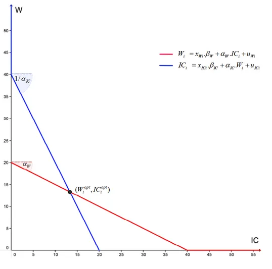
Considered independently, each equation refers to a partial equilibrium. The …rst equation (Wi = xW i: W+ W:ICiopt+ uW i) results from the …rst-order condition (3.4) which determines the
optimal working time conditionally on caregiving time (red curve in …gure 4). The second equation (ICi = xICi: IC + IC:Wiopt+ uICi) results from the …rst-order condition (3.5) which determines
the optimal caregiving time conditionally on working time (blue curve in …gure 4). With regard to the previous microeconomic framework, we expect W and IC to be both negative.
Considered simultaneously, both equations specify the optimal time allocation (Wiopt, IC opt i )
in the meaning that they de…ne a situation in which the individual has no incentive to deviate. In such a situation, the working time is optimal given caregiving time, while caregiving time is optimal given working time.
Model A is similar to the model proposed by Amemiya (1974) because we assume that each dependent variable is a function of the other observed dependent variable. It thus di¤ers from the model proposed by Nelson and Olson (1978) where each dependent variable is a function of the other latent dependent variable11. The choice of one or the other speci…cation is not neutral. It
depends on whether the theoretical economic model itself is simultaneous in the latent or observed dependent variables (Blundell and Smith, 1994). In the model proposed by Amemiya (1974), the
10A utility fonction leading to the reduced speci…cation 3.9 is for exemple : U
i(Ci; Li; ICi) = (Ci+ ZCi) :(Li+ ZLi) :(ICi+ ZICi) where , and are constant parameters and ZCi, ZLi and ZICi are linear functions of individual and family characteristics : ZCi= C+P Ck:xCki+ Ci, ZLi = L+P Lk:xLki+ Li and ZICi= IC+P ICk:xICki+ ICi. The coe¢ cients C, L, IC, Ck, Lk and ICkrepresent constant parameters while xCki, xLki, xICki, Ci, Li and ICi represent observed and unobserved (by the econometrician) individual and family characteristics.
11In the subsection 5.3, we presente estimation results from the Nelson and Olson speci…cation. The main conclu-sions are similar.
censoring mechanism acts as a constraint on agent’s behaviour, whereas in the model proposed by Nelson and Olson (1978) the censoring mechanism acts as a constraint on the information available to the econometrician but not on the agent’s behaviour itself. By choosing the model A, we assume, according to the previous theoretical model, that censoring mechanism a¤ects the agent’s decision making process. In others words, we consider for example that two non-workers, one characterized by a reservation wage slightly higher than the real wage and the other characterized by a reservation wage much higher than the real wage, will provide ceteris paribus the same amount of informal care.
Figure 4. Illustration of the optimal time allocation when (1 W: IC > 0)
Unlike the model proposed by Nelson and Olson (1978), model A may nevertheless present a risk of incompleteness in the sense that, for a given vector of exogenous variables (both observed and unobserved) it does not always predict a unique time allocation. This incompleteness stems from the fact that model A de…nes the optimal allocation as the intersection of two non linear
functions, one giving the optimal working time as function of caregiving time and the other giving the optimal caregiving time as function of working time.
As illustrated by …gures A1 and A2 in appendix A, this non linearity may potentially leads to several intersection points. In this case, the model predicts multiple equilibria. To overcome this di¢ culty, it is necessary to impose prior to estimating the model the following “coherence condition” (Maddala, 1983 ; Amemiya, 1974 ; Gourieroux et al., 1980) :
1 W: IC > 0 (3.10)
This condition ensures the completeness of the model whatever the individual (observed and unobserved) characteristics. In the subsection 5.3, we partially loosen this constraint by adding to the model a selection rule which allows to select a speci…c equilibrium in case of multiple equilibria (Krauth, 2006). Results are similar because the model still converges to a situation without multiple equilibria.
Note that the incompleteness characterizing this model is very di¤erent from the incomplete-ness charactering the model estimated by Fontaine et al. (2009) to study the interaction among siblings in their caregiving decisions. The theoretical model was itself incomplet in the sens that it de…ned the outcome (the observed care arrangement) as as Nash Equilibrium of a game that could potentially be characterized by no Nash equilibrium or by multiple equilibria. Here, things are di¤erent. The theoretical model is indeed "complet" because each individual is always cha-racterized by one and only one optimal time allocation. However, the econometric traduction of the theoretical model is incomplet because we de…ne in model A the optimal time allocation from the two …rst order conditions of the microeconomic model wich are necessary but not su¢ cient conditions to de…ne a equilibirum12.
Let P (Wi; ICi) = (Wiopt; IC opt
i ) denoted the probability for a given allocation to be optimal
12From this point of view, the estimation of a structural model would allow to compare the utility level associated with each possible equilibrium and then "complete" the model by adding a selection rule choosing the time allocation associated with the highest utility level. However, our reduced estimation does not allow to adopt this procedure.
for the individual i. For positive value of Wi and ICi, we have : P (Wi; ICi) = (W opt i ; IC opt i )
= P (uW i = Wi xW i: W W:ICi; uICi = ICi xICi: IC IC:Wi)
P (Wi; 0) = (W opt i ; IC opt i ) = P (uW i = Wi xW i: W; uICi< xICi: IC IC:Wi) P (0; ICi) = (W opt i ; IC opt i )
= P (uW i < xW i: W W:ICi; uICi= ICi xICi: IC)
P (0; 0) = (Wiopt; ICiopt)
= P (uW i < xW i: W; uICi < xICi: IC)
We assume that the residuals are distributed according to a bivariate normal density function : (uW i; uICi) N (0; 0; W; IC; ). Hence, the previous probabilities may be expressed as follow :
P (Wi; ICi) = (Wiopt; IC opt i ) = (1 W: IC):'(Wi xW i: W W:ICi; ICi xICi: IC IC:Wi) P (Wi; 0) = (Wiopt; IC opt i ) = Z xICi: IC IC:Wi 1
'(Wi xW i: W; uICi)duICi
P (0; ICi) = (Wiopt; IC opt i ) = Z xW i: W W:ICi 1
'(uW i; ICi xICi: IC)duW i
P (0; 0) = (Wiopt; ICiopt) = Z xICi: IC IC:Wi 1 Z xW i: W W:ICi 1
'(uW i; uICi)duW iduICi
where ' the joint density function of the bivariate normale.
The model can then be estimated with the maximum likelihood method. Here, we do not impose the coherence condition 1 W: IC > 0 during the estimation procedure but we verify a posteriori
that it is respected. Similarly, we do not impose the time constraint prior to the estimation but we verify, for each individual, that the estimations do not lead to a cumulated time devoted to work
and care exceeding 168 hours per week.
5.2 Results
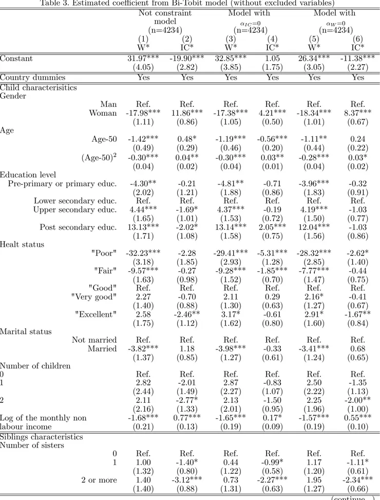
Columns (1)-(2) of table 3 reports our estimation results when we include the same explanatory variables in each equation. In this case, the identi…cation of the parameters is only due to the censure characterizing the working and caregiving time. The Appendix B reports estimation results when we reinforce the identi…cation by imposing exclusion restrictions. Speci…cally, we exclude from the working time equation siblings and parent’s characteristics and the number of children that is variables that empirically appear correlated with caregiving time but unrelated to working time (conditionally on the care provision). Symmetrically, we exclude from the caregiving time equation the marital status of the child and some modalities of his/her education level and health status that appear correlated with working time but unrelated to the caregiving time (conditionally on the working time). Results are however very similar.
As expected, the working time is negatively associated with the age and the non labour income but positively associated with the education level (column 1 of table 3). With regard to family network, being in couple signi…cantly reduces the labour supply whereas the number of children is not signi…cant. Moreover, the propensity to work is in‡uenced by the individual health status. Those declaring a “fair” or a “poor” health status present a lower propensity to work. Note that this variable may su¤er from an endogeneity bias since we do not control for the reversal causality, i.e. the impact of working behaviour on health status. Results remains however unchanged when we remove this variable from the estimation. Finally, none of the siblings and parent characteristics are signi…cant conditionally on time devoted to care.
Column (2) of table 3 reports the estimation results for the caregiving time equation. Woman, as expected, have a higher propensity to provide care than men. Providing care is also positively associated with the age and the non labour income and negatively associated with the education level. Moreover, those declaring an "excellent" health status have a lower propensity to provide care13. Being married has a no signi…cant e¤ect whereas the number of children reduces the
pro-pensity to provide care. The care provision is also a¤ected by the siblings’characteristics.
13As for the labour supply equation, this result may reveal the endogeneity of the healt status. Indeed, one can assume that the care provision negatively impact the health status of the caregiver.
Table 3. Estimated coe¢ cient from Bi-Tobit model (without excluded variables) Not constraint model (n=4234) Model with IC=0 (n=4234) Model with W=0 (n=4234) (1) W* (2) IC* (3) W* (4) IC* (5) W* (6) IC* Constant 31.97*** -19.90*** 32.85*** 1.05 26.34*** -11.38*** (4.05) (2.82) (3.85) (1.75) (3.05) (2.27)
Country dummies Yes Yes Yes Yes Yes Yes
Child characterisitics Gender
Man Ref. Ref. Ref. Ref. Ref. Ref.
Woman -17.98*** 11.86*** -17.38*** 4.21*** -18.34*** 8.37*** (1.11) (0.86) (1.05) (0.50) (1.01) (0.67) Age Age-50 -1.42*** 0.48* -1.19*** -0.56*** -1.11** 0.24 (0.49) (0.29) (0.46) (0.20) (0.44) (0.22) (Age-50)2 -0.30*** 0.04** -0.30*** 0.03** -0.28*** 0.03* (0.04) (0.02) (0.04) (0.01) (0.04) (0.02) Education level
Pre-primary or primary educ. -4.30** -0.21 -4.81** -0.71 -3.96*** -0.32
(2.02) (1.21) (1.88) (0.86) (1.83) (0.91)
Lower secondary educ. Ref. Ref. Ref. Ref. Ref. Ref.
Upper secondary educ. 4.44*** -1.69* 4.37*** -0.19 4.19*** -1.03
(1.65) (1.01) (1.53) (0.72) (1.50) (0.77)
Post secondary educ. 13.13*** -2.02* 13.14*** 2.05*** 12.04*** -1.03
(1.71) (1.08) (1.58) (0.75) (1.56) (0.86) Healt status "Poor" -32.23*** -2.28 -29.41*** -5.31*** -28.32*** -2.62* (3.18) (1.85) (2.93) (1.28) (2.85) (1.40) "Fair" -9.57*** -0.27 -9.28*** -1.85*** -7.77*** -0.44 (1.63) (0.98) (1.52) (0.70) (1.47) (0.75)
"Good" Ref. Ref. Ref. Ref. Ref. Ref.
"Very good" 2.27 -0.70 2.11 0.29 2.16* -0.41
(1.40) (0.88) (1.30) (0.63) (1.27) (0.67)
"Excellent" 2.58 -2.46** 3.17* -0.61 2.91* -1.67**
(1.75) (1.12) (1.62) (0.80) (1.60) (0.84)
Marital status
Not married Ref. Ref. Ref. Ref. Ref. Ref.
Married -3.82*** 1.18 -3.98*** -0.33 -3.41*** 0.68
(1.37) (0.85) (1.27) (0.61) (1.24) (0.65)
Number of children
0 Ref. Ref. Ref. Ref. Ref. Ref.
1 2.82 -2.01 2.87 -0.83 2.50 -1.35
(2.44) (1.49) (2.27) (1.07) (2.22) (1.13)
2 2.11 -2.77* 2.13 -1.50 2.25 -2.00**
(2.16) (1.33) (2.01) (0.95) (1.96) (1.00)
Log of the monthly non -1.68*** 0.77*** -1.65*** 0.17* -1.57*** 0.55***
labour income (0.21) (0.13) (0.19) (0.09) (0.19) (0.10)
Siblings characteristics Number of sisters
0 Ref. Ref. Ref. Ref. Ref. Ref.
1 1.00 -1.40* 0.44 -0.99* 1.17 -1.11*
(1.32) (0.80) (1.22) (0.58) (1.20) (0.61)
2 or more 1.40 -3.12*** 0.73 -2.27*** 1.95 -2.34***
(1.40) (0.88) (1.31) (0.63) (1.27) (0.66)
Table 3. Continue... Not constraint model (n=4234) Model with IC= 0 (n=4234) Model with W= 0 (n=4234) (1) W* (2) IC* (3) W* (4) IC* (5) W* (6) IC* Number of brothers
0 Ref. Ref. Ref. Ref. Ref. Ref.
1 0.82 -1.13 0.13 -1.14** 0.96 -0.99
(1.31) (0.80) (1.22) (0.58) (1.19) (0.60)
2 or more -0.93 -1.85** -1.63 -2.14*** -0.62 -1.56**
(1.39) (0.87) (1.29) (0.63) (1.26) (0.66)
Eldest child
No Ref. Ref. Ref. Ref. Ref. Ref.
Yes 0.77 0.69 0.59 0.79 0.60 0.65
(1.21) (0.75) (1.13) (0.54) (1.10) (0.57)
Parent characteristics Gender
Woman Ref. Ref. Ref. Ref. Ref. Ref.
Man -1.31 -2.36** -1.44 -2.06*** -1.08 -1.82** (1.58) (1.02) (1.46) (0.74) (1.44) (0.77) Age Age-75 0.16 0.47*** 0.12 0.39*** 0.00 0.36*** (0.13) (0.08) (0.12) (0.06) (0.11) (0.06) Health status
"Poor" Ref. Ref. Ref. Ref. Ref. Ref.
"Fair" -0.43 -3.00*** -0.16 -2.56*** 1.29 -2.55*** (1.54) (0.90) (1.46) (0.04) (1.40) (0.68) "Good" 2.40 -6.85*** 1.58 -5.11*** 4.54*** -5.54*** (1.61) (0.98) (1.54) (1.54) (1.45) (0.73) "Very good" 0.00 -9.08*** 0.04 -7.11*** 3.01 -7.29*** (2.21) (1.43) (2.10) (1.03) (2.00) (1.07) "Excellent" -1.66 -6.67*** -1.19 -5.55*** 1.23 -5.37*** (2.81) (1.78) (2.62) (1.18) (2.54) (1.33) Geographical proximity Same building -0.25 1.99 0.53 1.78 -1.51 1.85 (3.07) (1.69) (2.85) (1.20) (2.77) (1.23)
Less than 1km away Ref. Ref. Ref. Ref. Ref. Ref.
Between 1 and 5 km away -2.06 -4.76*** -1.55 -3.82*** 0.18 -3.88***
(1.87) (1.07) (1.76) (0.76) (1.69) (0.81)
Between 5 and 25 km away -0.75 -7.56*** -0.63 -6.01*** 1.77 -6.07***
(1.83) (1.08) (1.74) (0.77) (1.65) (0.81)
Between 25 and 100 km away -0.77 -11.02*** -0.23 -8.57*** 2.65 -8.52***
(2.02) (1.25) (1.92) (0.88) (1.81) (0.92)
Between 100 and 500 km away -0.52 -12.88*** -0.46 -10.27*** 2.85 -9.99***
(2.16) (1.40) (2.06) (0.99) (1.94) (1.03)
More than 500 km away -0.44 -18.54*** -0.83 -14.84*** 3.47 -14.17***
(3.46) (2.64) (3.27) (1.93) (3.13) (1.93)
More than 500 km away -1.76 -22.00*** -1.14 -17.14*** 1.81 -16.67***
in another coutry (3.01) (2.64) (2.83) (1.92) (2.74) (1.92)
Interactions between work and care
Hours of care (IC) -1.98*** -1.00*** .
(0.17) (0.20) .
Hous of work (W) 0.64*** . 0.42***
(0.04) . (0.04)
-0.53***(0.04) 0.15***(0.05) -0.64***(0.04)
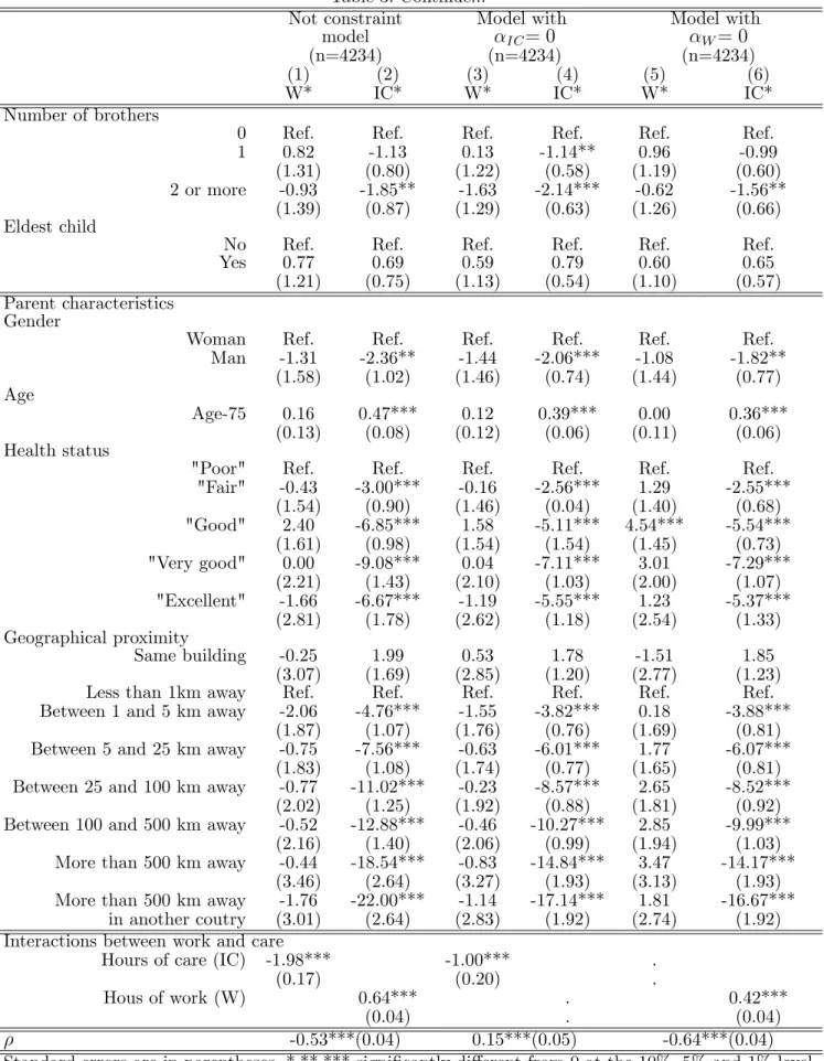
The number of brothers and number of sisters do not have the same impact on the caregiving behaviour : both have a negative and signi…cant impact on the propensity to provide care but, as expected, the propensity to provide care is more a¤ected by the number of sisters than the number of brothers. The siblings’ characteristics may reveal the existence of contextual interac-tions if the siblings’ characteristics (regardless their care provision) directly in‡uence individual caregiving behaviour, but may also reveal the presence of endogenous interactions, if the siblings’ characteristics act as proxies of the siblings’care provision (Manski, 2000). The model is however unable to disentangle this two mechanisms. Furthermore, being the elder child has a posititif but not signi…cant e¤ect on the propensity to provide care.
Regardless the parent’s characteristics, our estimation provides consistent results with the existing literature. In particular, the child’s care provision depends positively on the parent’s age and negatively on the parent’s health status. Our results also indicate that mothers receive signi…cantly more informal care than father14 and that children living further away from their
parents are characterized by a lower propensity to provide care than closer children15.
Turning now to the trade-o¤ between care and work, estimations results appear partially incon-sistent with our a priori expectations. More precisely, our results suggest that the care provision has a signi…cant negative impact on the propensity to work (bW = 1:98 ). This result is consistent
with the standard microeconomic model and the previous empirical litterature. However, the re-verse causality suggests that time spent working has a signi…cant positive impact on the propensity to provide care (bIC = 0:64 ).
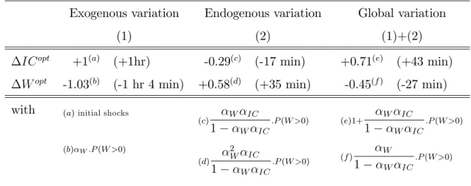
To investigate the intensity of these relations, we estimated the two reciprocal marginal e¤ects. We …rst estimate the e¤ect of a shock providing to each individual incentive to devote to parental care one more hour a week. Table 4 reports the optimal time allocation variation and a decom-position of this variation into an exogenous variation and an endogenous variation. The former
14In their structural model, Byrne et al. (2009) identify three mechanisms for the gender’s parent to in‡uence the care provision. Every things being equal, mothers and fathers may di¤er according to (i) health status, (ii) the burden associated with the care provision and …nally, (iii) the e¤ectiveness of the care provision. Their results provide some evidence that (i) fathers experience signi…cantly greater health status than mothers (caregiving marginal utility is thus higher for the child when he/she provides care for his/her mother rather his/her father), (ii) care provided for mothers is less burdensome than care provide for fathers and (iii) care provided for mothers is less e¤ective than care provide for fathers.
15The fact that geographical proximity could be endogenous was examined by Stern (1995). The endogeneity bias appears very limited.
supposes that the caregiving behaviour is exogenous in the sense that it does not depend on hours worked16. In the latter, the additional e¤ect induced by the endogeneity of the caregiving beha-viour is tacking into account. On average, the initial shock on time devoted to care produces a …nal decrease of working time by 28 minutes, whereas the optimal caregiving time, after adjustment, …nally increases by 43 minutes. The working time reduction is thus relatively high. At least three reasons may explain this e¤ect. First, the analysis is focused on individuals aged 50 to 65 that is a population for whom the caregiving behaviour may interact with the retirement decision. Some individuals may then leave the labour market in order to provide care for their disabled parent, in particular when others sources of care are not available. Following the decomposition proposed by McDonald and Mo¢ t (1980), we show that 49% of this the working time decrease (that is 13 minutes) comes from the decrease of the probability to work17. Second, individual labour behaviour
also depends on the labour demand, which is not taken into account in our model. In particular, if individuals may only choose between two work contracts (full time or part-time work), they may be constrained to reduce their working time more than they would in order to provide care for their parent. Finally, the depend variable considered here is the number of hours actually worked per week, not the basic or contractual hours (only relevant for employees). One can suppose that extra-contractual working hours are more a¤ected by caregiving behaviour than contractual hours. Similarly, Table 5 reports the optimal time allocation variation after a positive exogenous shock on the working time. After adjustment, the caregiving time variation appears relatively small (+5 minutes). Although the magnitude of the e¤ect is relatively small, the positif average e¤ect of working time on caregiving time calls into question the standard microeconomic framework used to think the interactions between time spent working and time devoted to parental care. Without going into speci…cs at this stage (this is the purpose of the next section), one can argue that this framework is quite restrictive because the interaction between working time and caregiving time does not directly involved the agent’s preferences but only the time constraint. In others words, through this model, if individuals were not constraint by time, the two activities would be independent.
16Through this e¤ect, we adopt a partial equilibrium perspective. One can see this e¤ect as the working time variation in a situation where the individual is virtually constraint to provide one more hour of care a week. Note that in this situation the time allocation is not optimal for the individual.
17The remaining 51% corresponds to the e¤ect on the time spent working conditionally on working. This decom-position is however constraint here by the fact that our model does not separately estimate the e¤ect of caregiving on the probability to work and on the number of hours worked conditionally on working.
Table 4 : Average e¤ect on an exogenous caregiving time variation on the optimal time allocation Exogenous variation (1) Endogenous variation (2) Global variation (1)+(2)
ICopt +1(a) (+1hr) -0.29(c) (-17 min) +0.71(e) (+43 min)
Wopt -1.03(b) (-1 hr 4 min) +0.58(d) (+35 min) -0.45(f ) (-27 min)
with (a)initial shocks
(c) W IC 1 W IC :P (W >0) (e)1+ W IC 1 W IC :P (W >0) (b) W:P (W >0) (d) 2 W IC 1 W IC :P (W >0) (f ) W 1 W IC :P (W >0)
Table 5 : Average e¤ect on an exogenous working time variation on the optimal time allocation Exogenous variation (1) Endogenous variation (2) Global variation (1)+(2)
Wopt +1(a) (+1hr) -0.17(c) (-10 min) +0.83(e) (+50 min)
ICopt +0.19(b) (+11 min) -0.11(d) (-7 min) +0.08(f ) (+5 min)
with (a)initial shocks
(c) IC W 1 IC W :P (IC>0) (e)1+ IC W 1 IC W :P (IC>0) (b) IC:P (A>0) (d) 2 IC W 1 IC W :P (IC>0) (f ) IC 1 IC W :P (IC>0)
To extend the comparison of our empirical results with those expected from the standard microeconomic model, we simulate speci…c shocks on the non labour income, on the parent’s health status and on the number of siblings. Consistently with our expectations, …ndings indicate …rst that a 1000 Euros increase of the monthly non labour income leads on average to a decrease in time spend working by 4 hours and 45 minutes a week and an increase in caregiving time by 25 minutes a week. Second, a deterioration of parent’s health status increases time devoted to care by 35 minutes a week on average whereas working time decreases by 25 minutes a week. Finally, having one more brother reduces caregiving time by 7 minutes a week and increases working time by 5 minutes a week whereas having one more sister reduces caregiving time by 12 minutes a week and increases working time by 8 minutes a week.
5.3 Robustness analysis
To check the robustness of our results, espcecially the positif e¤ect of an exogenous variation of working time on the propensity to provide care, we …rst partially relax the coherency condition. Situations with multiple equilibria may arise when the two parameters W and IC are both
negative and when the product W: IC is higher than 1. Three potential equilibrium may then
exist (one interior equilibrium and two corner equilibria, see …gure A.1 in appendix A ). In this case, we add to the model A (3.9) a selection rule which allows to select a particular equilibrium among the three potential equilibria (Krauth, 2006). Four di¤erent exogenous selection rules have been tested. The …rst assumes that each equilibrium has an equal probability (1/3) to be optimal and then chosen by the daughter. The three others assume than one of the three equilibria is always optimal and then always chosen by the child. See Bjorn and Vuong (1985), Fontaine et al. (2009), Krauth (2006), Soetevent & Kooreman (2007) or Tamer (2003) for similar approaches in a simultaneous discrete model. We still impose the coherency condition when the parameters
W and IC are both positive because in this case, individuals choose to increase their working and
caregiving time until that time devoted to leisure be equal to zero, which seems unrealistic (…gure A.2 in appendix A). Results obtained are strictly unchanged in comparison with those report in columns (1)-(2) of table 3 since the likelihood function still converges to the same value (each individual been characterized by a single equilibrium).
We have also compared our results with those obtained by an IV approach. We …rst estimated the following model :
Wiopt = 8 < : Wi if Wi > 0 0 otherwise and ICiopt = 8 < : ICi if ICi > 0 0otherwise (3.11) with 8 < : Wi = xW i: 0W + 0W:IC opt i + u0W i ICi = xICi: 0IC + xW i: 0W + u0ICi
The speci…cation of the working time equation is unchanged compared to model A (3.9). Ho-wever, contrary to previous model, the second equation is used to instrument the caregiving time. This approach is similar to the one used by Crespo (2007) and Johnson & La Sasso (2000), which only focus on the causal e¤ect of the caregiving time on the working time, that is on the parameter
0
W . Every variable which could directly or indirectly (through the working time) in‡uence the
care provision are included as explanatory variables in the caregiving time equation (the vector xICithen gathers the excluded instruments). The two equations are jointly estimated by maximum
likelihood method, allowing the residuals of the two equations to be correlated. Columns (3)-(4) of table 3 provides the estimation results without excluded instruments, the identi…cation being then only due the censures. Column (3)-(4) of table B1 (appendix B) provides the estimations results with excluded instruments. In both cases, the estimation results are very close from those obtained with the model A. In particular, the estimated e¤ect of an exogenous variation of caregiving time is still signi…cant (at the 1% level) and negative18. The marginal e¤ect is however slightly higher (in
absolute value) : on average, one more hour of caregiving decreases by 32 minutes working time.
The same approach is used to estimate the reverse causality. The model estimated is then the following : Wiopt = 8 < : Wi if Wi > 0 0 otherwise and ICiopt = 8 < : ICi if ICi > 0 0otherwise (3.12) with 8 < : Wi = xW i: 00 W + xICi: 0IC + u 00 W i ICi = xICi: 00 IC + 00 IC:W opt i + u 00 ICi
Estimation results provided by columns (5)-(6) of table 3 without excluded instruments and columns (5)-(6) of table B1 in appendix B with excluded instruments are also very close from those obtained with the model A : on average one hour more of working time increases time devoted to care by 7 minutes.
We have also distinguish the interactions according to child’s gender. The reciprocal e¤ects are in both cases slightly higher (in absolute value) for women but di¤erences are not signi…cant.
Finally, following the approach used by Boaz and Muller (1992), we have compared our results with those obtained from a speci…cation where we assume that the care provision and the labour supply interact through the latente variables rather than observed variables. We then estimate the
18Note also that, similarly to the previous literature, we …nd a positive correlation between the residuals of the two equations when we do not control for the direct e¤ect of labour supply on the care provision.
following model (Nelson and Olson, 1978) : model NO Wiopt= 8 < : Wi if Wi > 0 0 otherwise and ICiopt = 8 < : ICi if ICi > 0 0otherwise (3.13) with 8 < : Wi = xW i: W + W:ICi + uW i ICi = xICi: IC + IC:Wi + uICi
As Boaz and Muller (1992), we use the two step estimation procedure proposed by Nelson et Olson (1978). We …rst estimate a reduced form of the two equations and compute the predicted values of both latente variables. These predicted values, which are uncorrelated with the model’s error terms, are used to replace the endogenous RHS variables in the second stage equations. To allow the identi…cation of the parameters W and IC, we impose the same exclusion restrictions
than those used to estimate the model A. Table C1 (appendix C) provides estimation results. Findings are consistent with those obtained from model A : a positive exogenous variation of the propensity to provide care decreases the propensity to work whereas a positif exogenous variation of the propensity to work increases the propensity to provide care.
6 Microeconomic model with partial complementarity
The aim of this section is to propose a reformulation of the microeconomic model in order to account for the positif e¤ect (on average) of an positif exogenous working time variation on the optimal caregiving time.
6.1 How explain the positive e¤ect of an exogenous variation of working
time on the optimal caregiving time ?
The model proposed by Jonhson and La Sasso (2000) is only based on what the litterature called the "substitution e¤ect" (Carmichael and Charles, 1998). It comes from the time constraint : by devoting increasing time to a given activity, the agent is constraint to reduce the time available for other activities. Through this, working time and caregiving time appear as substitutes. However,
due to the agent’s preferences, other e¤ects may lead to a partial complementary between the two activites.
The …rst one is the “protection e¤ect”. Using results from a qualitative survey conducted in France among women providing support to their elderly parent, Le Bihan and Martin (2006) sug-gests that working is a protective activity for the caregivers. It allows them not to totally be absorbed by their caregiver activity. Unemployed individuals could therefore have a lower propen-sity to provide informal care for fear of not being able to limit their involvement, as the needs of the elderly parent increase. Among the children, we can asssume that this e¤ect is more relevant for daughters than sons if the duty to provide care to an elderly parent lie more heavily upon daughters than sons.
Two others e¤ect can also occur : the "respite e¤ect" and the "productivity e¤ect".
The "respite e¤ect" illustrates the fact that working may o¤er to the caregiver a way of freeing oneself from the emotional demands associated with the care provided for a relative (Carmichael & Charles, 1998). This e¤ect clearly appears in the declaration of a daughter who provides care to her elderly mother : "And it’s true that being at work, it helps to decompress and we are confronted with people who have had the same problem. So you can get advice. (...) Fortunately, there was the job ! Oh yes ! If there had not been the work ... "19 (from Le Bihan and Martin, 2006).
According to the “productivity e¤ect”, some occupations may allow the development of know-how that can be used in caregiving (personal care for a nurse, help with paperwork for bank employee). More generally, workers may be more inclined to accept a additional constaint on their schedule than retired people who may be more reluctant to loose some freedom on the use of their free time.
Through these three e¤ects, working appears as a factor increasing the propensity to provide informal care. Thus, they introduce into the analysis a kind of complementarity between the two activities. Speci…cally, theses e¤ects appear related to the worker status and not directly to the time spent working (conditionally on being a worker). To the best of our knowledge, they have never been integrated within a microeconomic model.
19"Et puis c’est vrai que d’être au boulot, ça aide quand même à décompresser et on se trouve confrontée à des personnes qui ont eu le même problème. Donc on peut avoir des conseils à droite et à gauche. (. . . ) Heureusement qu’il y avait le boulot ! Ah oui ! S’il n’y avait pas eu le travail. . . ".