HAL Id: hal-01378622
https://hal.inria.fr/hal-01378622
Submitted on 10 Oct 2016
HAL is a multi-disciplinary open access
archive for the deposit and dissemination of
sci-entific research documents, whether they are
pub-lished or not. The documents may come from
teaching and research institutions in France or
abroad, or from public or private research centers.
L’archive ouverte pluridisciplinaire HAL, est
destinée au dépôt et à la diffusion de documents
scientifiques de niveau recherche, publiés ou non,
émanant des établissements d’enseignement et de
recherche français ou étrangers, des laboratoires
publics ou privés.
A Quantitative Analysis of Cell Tower Trace Data for
Understanding Human Mobility and Mobile Networks
Neal Walfield, John Linwood Griffin, Christian Grothoff
To cite this version:
Neal Walfield, John Linwood Griffin, Christian Grothoff. A Quantitative Analysis of Cell Tower
Trace Data for Understanding Human Mobility and Mobile Networks. 6th International Workshop on
Mobile Entity Localization, Tracking and Analysis (MELT), Oct 2016, San Francisco, United States.
�10.1145/1235�. �hal-01378622�
A Quantitative Analysis of Cell Tower Trace Data
for Understanding Human Mobility and Mobile Networks
Neal H. Walfield
Johns Hopkins
John Linwood Griffin
Johns Hopkins
Christian Grothoff
INRIA
ABSTRACT
This paper provides insights into human mobility by analyz-ing cell tower traces. Cell tower trace data is an attractive method for studying mobility as the data can be collected in an energy-efficient and privacy-preserving way.
Our new data set is useful for confirming or determin-ing fundamental mobility parameters and for understanddetermin-ing mobile networks. In particular, we identify patterns in the data that would seem characteristic for particular behaviors, such as travel or work.
CCS Concepts
Networks → Network measurement; Human-centered computing → Empirical studies in ubiquitous and mobile computing;
Keywords
Cell tower trace, human mobility, user study
1.
INTRODUCTION
In this paper, we take a close look at a set of cell tower traces and identify interesting mobility patterns. Our goal is to provide quantitative properties of mobility data as well as to see which activities are likely recognizable in mobility trace data. Our focus is primarily descriptive. We identify, for instance, that the distribution of the number of times a tower is visited is consistent with a power law, and that users appear to sample the towers in their vicinity even though they are probably stationary. We also provide various vi-sualizations of the data from our mobility study that are helpful for understanding mobility data.
For our study, we collected 59 traces with at least 14 days worth of cell tower data from consenting volunteers using Nokia N900s from all over the world [17].1 High-resolution
1The data is set is available from http://hssl.cs.jhu.edu/
˜neal/woodchuck/user behavior study/ and CRAWDAD.
MELT 2016
ACM ISBN 978-1-4503-2138-9. DOI:10.1145/1235
trace data was collected on the device by listening to op-erating system events. The traces range from spanning the 14 day minimum to just under two years. We collected not only the currently connected cell tower (the focus of this analysis) and its signal strenth, but also recorded: periodic scans of Wi-Fi access points, data transfer statistics, the bat-tery’s charge as well as when and how it was charged, when the user interacted with the device, what programs the user ran, and when the device started and was shut down.
We were careful to not collect privacy-sensitive data. For instance, instead of recording each cell tower’s identifier, our logging program first obscured the cell id (CID) and the lo-cation area identifier (LAC) on the device itself. A conse-quence of this is that we cannot turn cell tower identifiers into geographic coordinates, which means that we cannot study the distribution of distances between visited locations. The reason for the focus on cell tower traces is that this method is power efficient. While the most straightforward way to obtain the current location is to use GPS, this would have placed a high load on the battery, and would not have worked well indoors on in urban canyons. Using cell tow-ers, we get globally unique identifitow-ers, determining a nearby tower does not require any extra energy, and coverage is nearly ubiquitous.
Prior studies of this type have been limited to a more bi-ased set of users [3, 11, 18], or were limited to certain activi-ties, e.g., driving a cab [10], or students while on campus [8]. We are only aware of one study, device analyzer, that pro-vides a larger and similarly diverse data set [15, 16], but this data set is not freely accessible and, as far as we know, has not yet been analyzed along this dimension. Other comple-mentary studies have looked at cell tower traces from the network operator’s perspective using call data records [6, 7, 9]. While these studies include millions of involuntary par-ticipants, they typically only have a few dozen records per participant per day, while we have virtually continuous cov-erage. Jiang et al., for instance, have under a 1000 records per user or just 24 records per day, on average [7].
2.
VISUALIZING MOVEMENT
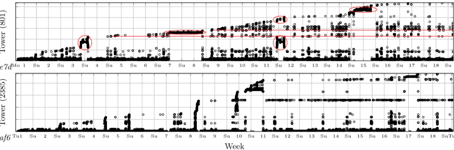
We visualize user movement by plotting the time that a user’s device connects to a tower vs. that tower’s identifier. We assign identifiers sequentially based on the time the user first connects to them. Because the first visit to a location or the first traversal of a route typically results in the discov-ery of most of the towers in the vicinity, this ordering should show the routes that the user traverses as steep, nearly ver-tical lines, and the places that the user visits as horizontal
Mo1 Su 2 Su 3 Su 4 Su 5 Su 6 Su 7 Su 8 Su 9 Su 10 Su 11 Su 12 Su 13 Su 14 Su 15 Su 16 Su 17 Su 18 Su T o w er (8 0 1 ) e7d Tu1 Su 2 Su 3 Su 4 Su 5 Su 6 Su 7 Su 8 Su 9 Su 10 Su 11 Su 12 Su 13 Su 14 Su 15 Su 16 Su 17 Su 18 SuTu Week T o w er (2 3 8 5 ) af6
Figure 1: The time the cell phone connects to a tower vs. tower identifiers. Towers are assigned identifiers according to the order in which the user first connects to them. The number in parenthesis is the total number of towers seen. The plots reveal that regime changes (moves, trips and changes in secondary activities) are common across users.
bands with the density of the band corresponding to how often the location is visited.
Fig. 1 shows the first 18 weeks of two representative traces. As expected we see near vertical lines, dark horizontal bands and what appear to be dashed and dotted horizontal lines. We speculate that these features correspond to the user’s home, movement, and regular activities, respectively. We assume that the dark bands correspond to the user’s home based on the time and duration of the users’ stays at these locations, and we use the label “home” accordingly.
We identify two important features. The first is the pres-ence of regime changes, which occur when the user visits a completely different set of towers for an extended period of time. A regime change is often temporary, and lasts from a few days to a few weeks. This pattern is seen in user e7d’s trace in weeks 3 and week 11 when the user goes away for the weekend, and in weeks 7 and 8 and in week 15 when the user goes away for about a week. These regime changes are circled in red on the plot. During these time periods, a new primary band is established, which, again, probably corresponds to where the user sleeps.
These trips are sometimes bookended by two nearly ver-tical lines, the first rising and the second falling. This is the case for the trips in week 3 and week 11 of user e7d’s trace. During the first trip, the user visits about 200 new towers. Most of these towers are visited twice, once at the beginning and once at the end of the trip, and form the two nearly vertical lines. The first vertical line means the user is visiting many new towers in quick succession. The near vertical line at the end of the trip is falling. This means that the user is traversing many towers in the opposite order of their discovery. That is, the user is taking the same route in reverse to go “home”. Note: going “home”, the user visits some new towers along the way: the segment of the graph actual looks more like alligator jaws: . This illustrates the second important feature: when traversing a known route, the actual set of towers that are visited varies.
During the second trip, the user visits many of the same towers (those in the lower circle) and again appears to use nearly the same route to travel to the destination and return “home”. The user also visits some new towers (those in the
upper circle) both while traveling and at the destination.
e7d af 6 d21 8b4 8b e 9ed 53 2 2ee 0b9 59 3 5cd 64 0 02 0 7e1 5a 9 99 e 87 e b37 c2b b84 1 3 6 10 18 32 56 100
Figure 2: The number of towers observed while the device is connected to a wall charger (not USB) for some represen-tative users.
These new towers appear to arise from the phone sampling the towers in its vicinity. To confirm this, we examined the number of towers that the cell phone observes while it is connected to a wall charger (not a USB port). In most such cases, we expect the device to be stationary. The exception is if the charger is connected to power while in a car or train. The results are shown in Fig. 2. Although the device often stays connected to a single tower, often times it connects to many different towers.
3.
TOWER VISITS
In this section, we examine tower visits: how long the participants in our study stayed at towers in total and during individual visits, and the number of visits as well as when those visits occur.
3.1
Tower Dwell Time
Fig. 3 shows complementary cumulative Pareto plots of the total time spent at a tower for several representative users. The x axis is the minimum number of visits, and the y axis is the number of towers for which this is the case. Thus, y(x = 1) is the number of towers that were visited at least once, the number of towers that were visited exactly once is y(2) − y(1), and the number of visits to the 10thmost
visited tower is y−1(10).
If data forms a straight line in a complementary cumula-tive Pareto plot, this is a sign that the data may be con-sistent with a power law [2]. Looking at the plots, we see that for most users, the data forms a roughly straight line
1s 7s 55s 7m 50m 6h 45h 14d15w 1 3 10 32 100 320 1 k 6.2 k Days: 605 α = 1.67 xmin = 38m p-value = 0.816
Minimum Dwell Time
Nu m b er of T o w e rs e7d 1s 7s 55s 7m 50m 6h 45h 14d15w 1 3 10 32 100 320 1 k 6.5 k Days: 523 α = 1.62 xmin = 2m p-value = 0.000
Minimum Dwell Time
af6 1s 7s 55s 7m 50m 6h 45h 14d15w 1 3 10 32 100 320 1 k 5.2 k Days: 514 α = 1.53 xmin = 43s p-value = 0.022
Minimum Dwell Time
d21 1s 7s 55s 7m50m 6h 45h14d15w 2y 1 3 10 32 100 320 1.6 k Days: 433 α = 1.82 xmin = 46m p-value = 0.064
Minimum Dwell Time
8b4 1 2 3 4 5 6 7 8 9 101112131415 0% 20% 40% 60% 80% 100% 20 10 95 53 3 2 22 2 1 1 11 Towers: 6292 Days: 605 Top Towers T o ta l Time e7d 0% 1 2 3 4 5 6 7 8 9 101112131415 20% 40% 60% 80% 100% 25 205 54 333 2 2 22 21 1 Towers: 6658 Days: 523 Top Towers af6 0% 1 2 3 4 5 6 7 8 9 101112131415 20% 40% 60% 80% 100% 38 8 7 74 3 32 2 2 22 1 1 .7 Towers: 6182 Days: 514 Top Towers d21 0% 1 2 3 4 5 6 7 8 9 101112131415 20% 40% 60% 80% 100% 774 2 2 1 .6 .4 .4 .3 .3 .3 .2 .2 .2 .2 Towers: 1625 Days: 433 Top Towers 8b4
Figure 3: Complementary cumulative Pareto plots of the minimum total time spent at a tower and the portion of time spent at the top 15 towers (ranked by time spent at the tower) vs. the cumulative portion of the total time connected to the top towers. The numbers near the top of the bars indicate the portion of time spent at that tower (not cumulative). The plots illustrate that the top few towers dominate in terms of the amount time the user spends at them. Of the 59 traces, 44 of the fits to a power law (75.0%) are significant at the p = 0.05 level with an average α of 1.60, and a standard deviation of 0.15.
starting with dwell times that exceed a few minutes and has a minor, downward deviation on the right.
To determine whether the data is consistent with a power law, we used Clauset et al.’s methodology to fit the data and to compute the goodness of fit [2]. Even without ex-plicitly accounting for the deviation in the tail, we find that 44 of the 59 traces (75.0%) are consistent with a power law at the p = 0.05 level, which suggests that this power law behavior is common. Further, all of the data have similar parameters: the average value of α is 1.60 with a modest standard deviation of 0.15. And, the median xminis 3
min-utes (170 seconds) with a median absolute deviation (MAD) of 3 minutes (203 seconds).
To better understand the implications of the power law behavior, we also plotted the portion of time spent at the top 15 towers. We excluded all tower visits that are longer than two days to avoid inflating the amount of influence that the top towers have. (There are 47 such visits across 11 users.) We assume in these cases that the user forgot her cell phone at home, for instance.
Even with these extreme cases removed, the data shows that all users spend at least two-thirds of their time at their top 15 towers, and most of them spend over 80% of their time there. To keep this in perspective, most users visit hundreds or thousands of towers over the course of their trace (the exact number is shown in an inset). In other words, the top 15 towers account for 80% of the time, but correspond to only 1% of the towers that a user ever visits.
3.2
Visit Dwell Times
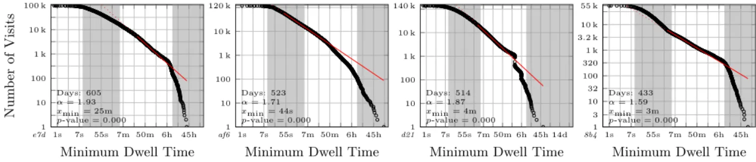
We now look at the duration of tower visits, i.e., the amount of time spent at a tower during an individual visit. Fig. 4 shows complementary cumulative Pareto plots of the duration of tower visits. The x axis shows the minimum
dwell time and the y axis shows the number of visits for which this is the case. We see that the middle part of the data—between about 3 minutes and 12 hours—roughly fol-lows a straight line, however, the left side of the plots and the tails exhibit strong deviations. The practical result of the upper deviation is that few of the traces are consistent with an untruncated power law distribution: of the 59 traces, only 18 (31.0%) follow a power law at the p = 0.05 level. In fact, it is primarily the traces with at most 3 months of data for which a power law is a significant fit. In these traces, the deviation on the right is probably indistinguish-able from noise. (The average value of α for all 59 traces is 1.86 with a standard deviation of 0.24.)
A close look at the data suggests four different behaviors depending on the dwell time. These regions are demarcated in the plots by gray bands in the background.
The first region consists of dwell times that are less than about 10 or 20 seconds long. In this region, there are far fewer visits with these dwell times than would be predicted by the regression. This is not surprising. If the user needs to traverse 1000 feet of a cellular tower’s area before chang-ing to a new tower, the user would need to travel at nearly 70 miles per hour to complete the traversal in 10 seconds. In places where a user can travel that fast, e.g., along a high-way, the towers will be laid out to avoid too many handoffs, i.e., the typical traversal will be longer, making such a fast traversal unlikely. Thus, a lower cutoff of at least 10 sec-onds and a correspondingly sharp drop in the number of short visits, as observed in the plots, is reasonable.
The next region is from about 10 seconds up to approx-imately 3 minutes. Many of the visits in this region likely correspond to user movement: these dwell times correspond to the dwell times along long chains of towers (not shown), which we speculate are routes.
1s 7s 55s 7m 50m 6h 45h 1 10 100 1 k 10 k 100 k Days: 605 α = 1.93 xmin = 25m p-value = 0.000
Minimum Dwell Time
Nu m b er of Vis it s e7d 1 1s 7s 55s 7m 50m 6h 45h 10 100 1 k 10 k 120 k Days: 523 α = 1.71 xmin = 44s p-value = 0.000
Minimum Dwell Time
af6 1 1s 7s 55s 7m 50m 6h 45h 14d 10 100 1 k 10 k 140 k Days: 514 α = 1.87 xmin = 4m p-value = 0.000
Minimum Dwell Time
d21 1 1s 7s 55s 7m 50m 6h 45h 3 10 32 100 320 1 k 3.2 k 10 k 55 k Days: 433 α = 1.59 xmin = 3m p-value = 0.000
Minimum Dwell Time
8b4
Figure 4: Complementary cumulative Pareto plots of the time spent during each tower visit. 18 of the fits to a power law (31.0%) are significant at the p = 0.05 level. The average α is 1.86, with a standard deviation of 0.24.
Dwell times in the region between 3 minutes and about 10 to 12 hours primarily correspond to the locations that users visit. For most users, these dwell times appear to follow a power law as can be seen from the roughly straight line that the data forms in the CCDF plots.
The final region starts at between 10 and 12 hours and also appears to roughly follow a straight line. This line, however, is much steeper than the previous one. This region consists of a very small portion of the total tower visits: the median number of visits that are at least 10 hours long is just 13% of the total number of days that the corresponding trace covers! This consistent drop in the number of visits is likely due to diurnal effects: most people leave the house every day whether it is to go to work or to do some errands. Some of the visits in this region are extremely long. For instance, in user d21’s trace, we see several visits to a tower for multiple weeks! Plausible reasons for such long visits include the user leaving the cell phone at home or being too sick to move.
3.3
Visit Dwell Times by Tower
We now examine the visit dwell time broken down for the most significant towers, those at which the users spend the most time. Fig. 5 shows e7d’s top four towers in terms of the total time spent there. Each plot is a histogram of the amount of time spent during each visit to the tower. The x axis is the same for all plots to facilitate comparisons across towers. The number at the bottom of each bar indicates the portion of the total time spent at this tower that the visits in this range constitute.
Information about the towers is inset in the plots. The first line shows the total amount of time spent at the tower and the tower’s rank according to this metric. This is fol-lowed by the total number of visits and the tower’s rank ac-cording to this metric. Then, the number of days on which the tower is visited at least once is shown. Finally, the me-dian number of visits per day for days on which the tower is visited at least once is displayed as well as the corresponding median absolute deviation.
A close look at the data reveals that in nearly all cases the mode is less than about 7 minutes. In other words, short visits dominate even for the towers that users spend the most time at. In terms of the amount of time spent at a tower, however, long visits generally dominate. Con-sider, for instance, e7d’s top tower: 68% of the visits are less than 10 minutes long. However, visits longer than an hour account for nearly 90% of the time spent at the tower. This distribution is surprising if we assume a fixed
loca-tion is generally covered by a single tower. It is, however, explained if we assume that cell phones sample the towers in their vicinity, a hypothesis that is also supported by the alligator jaws we saw in Fig. 2.
The most important towers are typically visited a few times per day. However, there are many towers that are visited dozens of times per day. This is the case for af6’s top tower (not shown), which is visited more than 40 times per day! Such towers are most likely involved in oscilla-tions where the phone constantly switches between two tow-ers. This is likely because the location is on the border of two cells, i.e., a location in which the two strongest cell towers have a similar signal strength.
3.4
Number of Tower Visits
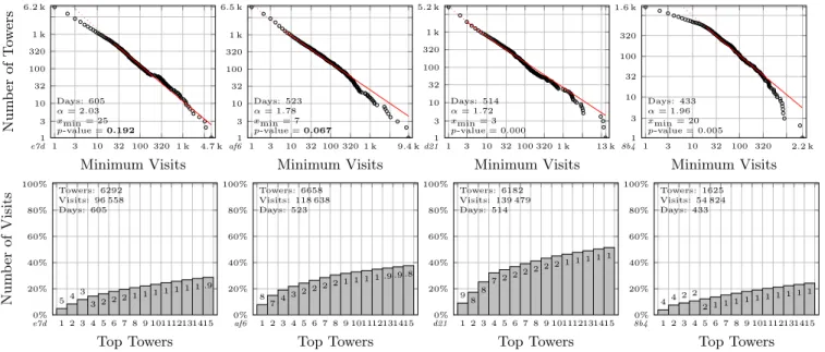
We now consider how many times each tower is visited. Fig. 6 shows complementary cumulative Pareto plots of the number of tower visits. The x axis shows the minimum number of times the user visited a tower and the y axis shows the number of towers for which this is the case. The plots in the second row show CDFs of the number of times the top tower towers are visited.
In many of the plots in Fig. 6, the data roughly follows a straight line. There is some minor downward deviation on the left side and some more significant downward deviation in the tail. However, even without explicitly accounting for the deviation in the tail, we find that 35 of the 59 traces (59.0%) are consistent with a power law at the p = 0.05 significance level. Further, all of the traces have similar pa-rameters: the average value of α across all 59 traces is 1.84 with a modest standard deviation of 0.22. This suggests that this particular power law behavior may be common.
The deviation on the left—when there is one—is almost always downward. Based on the selection of xmin, we see
that the deviation is relatively small: the median value of xminis 6 with a MAD of 6. The downward deviation means
that fewer towers are visited at most a handful of times than the model predicts. Nevertheless, the number of towers with only a few visits is enormous: the median portion of towers with at most three visits is 58.1% (MAD: 13.2%). Interestingly, these towers correspond to just 1.0% of the total time on average (MAD: 0.74%).
Based on the number of visits to these towers, and the total amount of time spent connected to them, these towers are probably along routes that are rarely taken. In practice, the longest of these routes probably do not actually have any cell towers: very long distance trips are more conveniently made by airplane than by car or train and a cell phone’s
1s 7s 55s 7m 50m 6h 45h 0 100 200 300 400 514 0% 0% 0% 0% 0% 1% 2% 5% 11 % 20 % 38 % 23 % Time: 17.4 w (20%, #1) Visits: 3255 (3.4%, #3) Days w/Visits: 295 (49%) Visits per Day: 9 (5.93)
Dwell Time Nu m b er of Vis it s 19 1s 7s 55s 7m 50m 6h 45h 0 50 100 150 200 250 300 345 0% 0% 0% 0% 1% 2% 3% 10 % 15 % 16 % 51 % 2% Time: 8.6 w (10%, #2) Visits: 2448 (2.5%, #4) Days w/Visits: 213 (35%) Visits per Day: 11 (5.93)
Dwell Time 2612 1s 7s 55s 7m 50m 6h 45h 0 100 200 300 400 529 0% 0% 0% 0% 0% 0% 1% 3% 6% 13 % 75 % 2% Time: 7.5 w (8.8%, #3) Visits: 1697 (1.8%, #6) Days w/Visits: 277 (46%) Visits per Day: 5 (2.97)
Dwell Time 26 1s 7s 55s 7m 50m 6h 45h 0 50 100 150 200 250 332 0% 0% 0% 0% 1% 0% 1% 4% 5% 15 % 73 % Time: 4.3 w (5.1%, #4) Visits: 1217 (1.3%, #9) Days w/Visits: 207 (34%) Visits per Day: 5 (2.97)
Dwell Time
2615
Figure 5: Visit dwell time histogram for e7d’s top towers. The number at the bottom of each bar is the portion of time that the visits constitute. Inset in each figure are the total time and total visits to the tower as well as the number of days with visits and the median visits per day for days on which the tower was visited at least once and the corresponding MAD.
1 3 10 32 100 320 1 k 4.7 k 1 3 10 32 100 320 1 k 6.2 k Days: 605 α = 2.03 xmin = 25 p-value = 0.192 Minimum Visits Nu m b er of T o w e rs e7d 1 3 10 32 100 320 1 k 9.4 k 1 3 10 32 100 320 1 k 6.5 k Days: 523 α = 1.78 xmin = 7 p-value = 0.067 Minimum Visits af6 1 3 10 32 100 320 1 k 13 k 1 3 10 32 100 320 1 k 5.2 k Days: 514 α = 1.72 xmin = 3 p-value = 0.000 Minimum Visits d21 1 3 10 32 100 320 2.2 k 1 3 10 32 100 320 1.6 k Days: 433 α = 1.96 xmin = 20 p-value = 0.005 Minimum Visits 8b4 1 2 3 4 5 6 7 8 9 101112131415 0% 20% 40% 60% 80% 100% 54 3 3 22 21 1 1 1 1 11 .9 Towers: 6292 Visits: 96 558 Days: 605 Top Towers Nu m b er of Vis it s e7d 1 2 3 4 5 6 7 8 9 101112131415 0% 20% 40% 60% 80% 100% 8 74 3 22 2 2 1 11 1 .9.9 .8 Towers: 6658 Visits: 118 638 Days: 523 Top Towers af6 1 2 3 4 5 6 7 8 9 101112131415 0% 20% 40% 60% 80% 100% 9 8 8 7 22 2 2 22 1 1 1 11 Towers: 6182 Visits: 139 479 Days: 514 Top Towers d21 1 2 3 4 5 6 7 8 9 101112131415 0% 20% 40% 60% 80% 100% 44 2 2 2 11 1 1 1 1 11 1 1 Towers: 1625 Visits: 54 824 Days: 433 Top Towers 8b4
Figure 6: Complementary cumulative Pareto plots of the number of times a tower is visited (the x axis is the minimum number of times a tower is visited, and he y axis is the number of towers for which this is the case) and the top towers (according to the number of times they are visited) vs. the cumulative portion of total visits. The top few towers dominate. The number at the top of each bar corresponds to the portion of visits (not cumulative) to that tower. 35 of the fits to a power law (59.0%) are significant at the p = 0.05 level. Of the 59 fits, the average α is 1.84, with a standard deviation of 0.22.
radio is often turned off while in the air. This lack of cell towers during flights may explain the downward deviation.
The deviation in the tail is also generally downwards. The towers in this region correspond to those few towers that users connect to many times, which are probably those near where the participants live and work. In fact, even though users visit thousands of different towers, the median portion of tower visits to the top 15 towers is 57.0% (MAD: 21.0%). Taking a close look at Fig. 6, we see that each user’s most visited tower is visited thousands of times over the course of the trace (median: 2830, MAD: 2940). On average, this works out to dozens of visits per day (median: 28, MAD: 19). In fact, the most visited tower is visited 67 017 times (user: 9ed), which translates to 180 connections on average per day. What is actually happening here is that the user’s cell phone is oscillating between two towers. We already observed this phenomenon in Sec. 3.3.
4.
TOWER TRANSITIONS
We now examine tower transitions on the induced cell tower network. It would have also been reasonable to use cell tower co-occurrence, as in [4]; however, the target platform for our study did not support collecting co-occurrence data.
4.1
Transition Directions
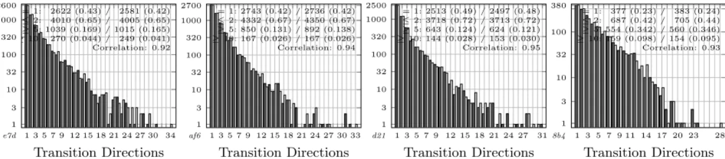
Fig. 7 shows histograms of the towers’ outgoing and in-coming transition directions for the top four participants. A transition direction is an edge in the induced cell tower network. For example, if we observe that a user transitions from tower a to tower b 100 times and from tower a to tower c 50 times, then we have identified two edges, two outgoing transition directions (a → b and a → c) and two incoming transition directions (b ← a and c ← a). The inset in each plot shows the number of towers with selected in or out de-grees as well as the correlation between in degree and out degree.
1 3 5 7 9 12 15 18 21 24 27 30 34 1 3 10 32 100 320 1000 2600 = 1: 2622 (0.43) / 2581 (0.42) ≤ 2: 4010 (0.65) / 4005 (0.65) ≥ 5: 1039 (0.169) / 1015 (0.165) ≥ 10: 270 (0.044) / 249 (0.041) Correlation: 0.92 Transition Directions Nu m b er of T o w e rs e7d 1 3 5 7 9 12 15 18 21 24 27 30 33 1 3 10 32 100 320 1000 2700 = 1: 2743 (0.42) / 2736 (0.42) ≤ 2: 4332 (0.67) / 4350 (0.67) ≥ 5: 850 (0.131) / 892 (0.138) ≥ 10: 167 (0.026) / 167 (0.026) Correlation: 0.94 Transition Directions af6 1 3 5 7 9 12 15 18 21 24 27 31 1 3 10 32 100 320 1000 2500 = 1: 2513 (0.49) / 2497 (0.48) ≤ 2: 3718 (0.72) / 3713 (0.72) ≥ 5: 643 (0.124) / 624 (0.121) ≥ 10: 144 (0.028) / 153 (0.030) Correlation: 0.95 Transition Directions d21 1 3 5 7 9 11 14 17 20 23 28 1 3 10 32 100 380 = 1: 377 (0.23) / 383 (0.24) ≤ 2: 687 (0.42) / 705 (0.44) ≥ 5: 554 (0.342) / 560 (0.346) ≥ 10: 159 (0.098) / 154 (0.095) Correlation: 0.93 Transition Directions 8b4
Figure 7: Histogram of outgoing (dark left bar) and incoming (light right bar) tower transition directions. A tower a has the two outgoing transition directions a → b and a → c if, when at tower a, the user only ever transitions to tower b or tower c.
The histogram does not show the relationship between the number of outgoing and incoming transition directions. However, the correlation between the number of outgoing and incoming transition directions is significant. The mean correlation coefficient for the 59 traces is 0.92 with a stan-dard deviation of 0.024. (Note: a correlation whose magni-tude exceeds 0.7 is considered to be strong [1].) Given the large number of towers with just a single transition direc-tions, we checked if the the correlation remains strong even if we only consider towers that have at least three incoming or outgoing transition directions. It does: the mean correlation is 0.86 with a standard deviation of 0.060.
We can roughly divide the towers into three types: towers with at most three incoming or outgoing transitions direc-tions; those with more than 10 incoming or outgoing transi-tion directransi-tions; and those that are in between.
Towers with no more than a few transition directions are the most common. On average, 70% of the towers have no more than three incoming or outgoing transition directions (standard deviation: 12%). We speculate that these towers typically correspond to routes taken by the user.
Based on our sampling hypothesis, the middle group is what we intuitively expect for towers at significant fixed lo-cations: the user transitions between most pairs of towers as she moves around the area. Since cells are approximately laid out in a hexagonal tessellation, we expect a given cell tower to have at most 6 neighbors. However, a cell is often subdivided into 2 to 6 sectors using multiple sector anten-nas instead of a single omni-directional antenna [12]. When dividing cells in this way, each sector is given its own unique identifier and thus appears as a unique cell. Further, a cell may be subdivided into smaller cells. If the neighboring cells are sectored or subdivided, it is conceivable that a given cell could have about a dozen immediate neighbors.
The last group consists of towers with more than 10 tran-sition directions. These account for 4.2% of the towers, on average (standard deviation: 3.7%). These typically corre-spond to the towers the user visits most frequently, as we find that there is a high correlation (median Spearman cor-relation coefficient: 0.9; MAD: 0.028) between the number of times a tower is visited and its out-degree. This suggests that interference causes the modem to sample towers that are far away.
The distribution of the number of transition directions per tower appears to be distributed according to a right heavy-tailed distribution: we have many towers with just a few transition directions and a non-negligible number with a huge number of transition directions. However, none of the common distributions (power law, left-truncated
expo-nential or log normal) seem reasonable.
4.2
Transition Direction Popularity
We now investigate transition direction popularity, i.e., how often each transition direction is taken.
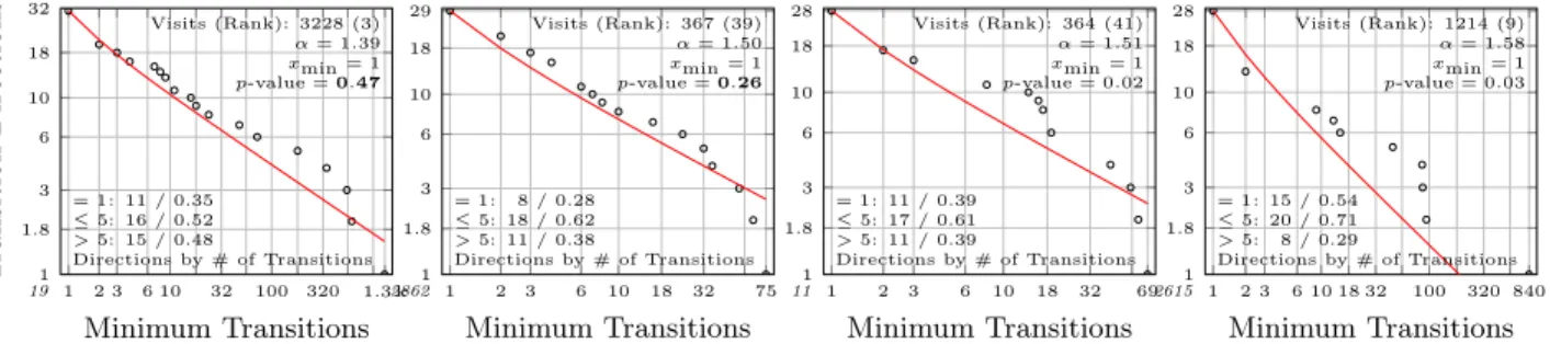
Fig. 8 shows a complementary cumulative Pareto plot of the number of times each outgoing transition direction is taken for the top 4 towers (according to the number of out-going transition directions) for the top trace.
The first thing to notice is that the number of times a transition direction is taken is not uniformly distributed. Rather, half of the transition directions are taken at most a handful of times, some are taken occasionally, and a few dominate.
This distribution suggests that how often a transition di-rection is taken is distributed according to a right heavy tailed distribution. To confirm this, we fit the data for each tower with at least 15 transition directions to a power law, which is also shown in Fig. 8. There are 915 such towers across all of the traces. Tbl. 1 summarizes the findings. The summary statistics for the α are calculated using just the statistically significant results.
The table reveals that the fit is generally statistically sig-nificant: for 91% of the towers, the fit of the popularity of the transition directions to a power law is significant at the p = 0.05 level. Moreover, the value of α is similar across towers and traces: the mean value of the αs is 1.71 with a standard deviation of 0.330. Note: in terms of evaluating the fit, the number of transition directions is relatively small and the fit could partially be a product of overfitting.
This result suggests that although some towers have many transition directions, most of them are unimportant and can generally be ignored. This should simplify predicting a tower’s successor even if it has ten or twenty transition directions: only a few are common.
4.3
Discussion
When looking at transition direction popularity, we found that half of the tower transitions are taken at most a handful of times. If we ignore these transition directions, the 4.2% of towers with more than 10 transition directions shrinks dramatically. We refer to these transition directions as rare transition directions. They are rare not because they occur infrequently (indeed, they are very common), but because they are taken infrequently. We now consider reasons for the large number of transition directions observed at some towers. All of these reasons also contribute to the tower sampling, which we previously observed.
di-1 2 3 6 10 32 100 320 1.3 k 1 1.8 3 6 10 18 32 = 1: 11 / 0.35 ≤ 5: 16 / 0.52 > 5: 15 / 0.48 Directions by # of Transitions Visits (Rank): 3228 (3) α = 1.39 xmin = 1 p-value = 0.47 Minimum Transitions T ra n si ti o n Direct ion s 19 1 1 2 3 6 10 18 32 75 1.8 3 6 10 18 29 = 1: 8 / 0.28 ≤ 5: 18 / 0.62 > 5: 11 / 0.38 Directions by # of Transitions Visits (Rank): 367 (39) α = 1.50 xmin = 1 p-value = 0.26 Minimum Transitions 2862 1 1 2 3 6 10 18 32 69 1.8 3 6 10 18 28 = 1: 11 / 0.39 ≤ 5: 17 / 0.61 > 5: 11 / 0.39 Directions by # of Transitions Visits (Rank): 364 (41) α = 1.51 xmin = 1 p-value = 0.02 Minimum Transitions 11 1 1 2 3 6 10 18 32 100 320 840 1.8 3 6 10 18 28 = 1: 15 / 0.54 ≤ 5: 20 / 0.71 > 5: 8 / 0.29 Directions by # of Transitions Visits (Rank): 1214 (9) α = 1.58 xmin = 1 p-value = 0.03 Minimum Transitions 2615
Figure 8: Complementary cumulative Pareto plot of the popularity of outgoing transition directions for the top towers (according to the number of outgoing transition directions) in user e7d’s trace.
rections is due to interference. Schwartz observes that if a receiver moves just half of a wave length—21.4 cm for 700 MHz radio waves and 7.5 cm for 2 GHz radio waves— the signal “may vary many dB” due to multipath fading, which is “the destructive/constructive phase interference of many received signal paths” [12, Section 2.2]. Thus, it is likely that the nearby towers sometimes appear to be rela-tively weak and a distant tower appears to be strong.
This is compounded by the layout of networks. First, a cell tower often does not cover a circular region, but a cone due to sectoring. Further, as cells become smaller (to increase capacity), overlap increases.2
Umbrella cells also increase the number of logical neigh-bors. An umbrella cell is a macrocell that overlays a group of microcells [5,14]. An example is shown in Fig. 9. The cel-lular concept is based on fractals: if the system needs more capacity, instead of using more spectrum, a cell is split into a number of smaller cells, say 7, and each is configured to transmit with just enough power to cover 1/7 of the area.
This results in (ideally) a 7 fold increase in the amount of capacity in the area. The most obvious additional costs of splitting a cell are the additional equipment, their mainte-nance and the rent for the new locations’ real estate. There is, however, another cost: cellular stations need to change towers more often when moving. The umbrella cell reduces this overhead: when a station starts to move, instead of connecting to the neighboring microcell, it connects to the umbrella cell. When it is stationary and again needs to transmit, it may switch back to a microcell.
Umbrella cells are a possible cause of the numerous transi-tion directransi-tions that many cell towers have: the user can tran-sition not only to the umbrella cell’s neighbors, but to any of the umbrella cell’s microcells. Many of these transition directions are likely to be infrequent. For instance, when the user moves from A to B in Fig. 9, he might not immediately transition to M upon leaving A: the handoff to the
um-2If the lower limit at which a cell phone can communicate
with a cell tower is -100 dBm, then we do not want to con-figure the tower such that the expected signal at its border is -100 dBm. This would result in dead spots if there was interference. Instead, we might aim for, say, -90 dBm. Since the distance that it takes -100 dBm to decay to -90 dBm is the same (ignoring interference) independent of how far away the source is or how strong the signal initially was, smaller cells will overlap more than larger cells. That is, if there is minimal overlap when a cell’s radius is r, then when r is increased by δ, the cell overlaps approximately π (r + δ)2− πr2 with its neighbors. Thus, the ratio of the
overlap to its area (π(r+δ)2−πr2
/πr2) shrinks as r increases.
M
A
B
Figure 9: An umbrella cell tower with 10 microcells. Note: the microcells need not completely fill the umbrella cell; they only need to be deployed where additional capacity is needed. In such a configuration, moving from A to B could result in the following tower sequence A → M → B.
A B
C
Figure 10: Although towers A and C are not adjacent, it is conceivable that the user could transition directly from A to C if B is overloaded and refuses a handoff. In this situation, the user could still remain connected to A until it reaches C: A and B do not interfere, because they use different frequencies; A’s reception will, however, be weak.
brella cell only happens if the user appears to have reached a velocity that suggests longer movement. Thus, he might first connect to the right neighboring cell and then to M . Another possibility is that the user is transferring data and the station switches to a microcell when the user is at a stop light, because it has more capacity than the umbrella cell.
The phone may also behave slightly different when it has an active connection to the network. For instance, if the strongest tower is refusing handoffs, perhaps because it is overloaded [13, Sect. 7.12.3], then the phone may appear to make a large jump, as shown in Fig. 10.
Finally, firmware bugs and bugs in our logging software as well as changes to the network layout could also result in these rare transition directions.
5.
CONCLUSION
We have presented results from a mobility study using cell tower trace data and have illustrated how the collected data could be used to identify various patterns of life. In future work, we plan to use the data set to evaluate context prediction algorithms.
Towers α
User Time Total p ≥ 0.05 µ σ
e7d 85.4 w 62 56 / 90% 1.73 0.311 af6 73.7 w 44 38 / 86% 1.70 0.370 d21 77.8 w 39 35 / 90% 1.65 0.316 8b4 61.4 w 28 27 / 96% 1.76 0.393 8be 57.3 w 62 56 / 90% 1.74 0.389 532 51.4 w 43 40 / 93% 1.69 0.317 715 33.3 w 55 47 / 85% 1.77 0.377 2ee 46.1 w 4 4 / 100% 1.77 0.386 0b9 31.9 w 33 31 / 94% 1.66 0.258 593 34.9 w 5 5 / 100% 1.49 0.177 5cd 32.1 w 11 11 / 100% 1.93 0.633 640 26.5 w 99 86 / 87% 1.78 0.335 020 28.3 w 39 31 / 79% 1.75 0.356 7e1 27.1 w 1 1 / 100% 1.36 — 5a9 20.4 w 38 37 / 97% 1.60 0.357 99e 22.5 w 64 62 / 97% 1.67 0.278 87e 19.4 w 50 45 / 90% 1.75 0.300 b37 16.5 w 12 10 / 83% 1.90 0.323 c2b 17.3 w 21 20 / 95% 1.77 0.341 b84 16.8 w 15 15 / 100% 1.55 0.210 935 17.5 w 20 15 / 75% 1.67 0.175 bb7 16.3 w 10 9 / 90% 1.59 0.317 f14 16.2 w 28 25 / 89% 1.75 0.330 26c 14.3 w 21 21 / 100% 1.86 0.309 9cf 7.4 w 5 4 / 80% 1.58 0.0738 05b 11.6 w 7 7 / 100% 1.60 0.142 c5d 10.5 w 3 3 / 100% 1.54 0.172 b7e 12.6 w 22 20 / 91% 1.74 0.307 772 9.6 w 1 1 / 100% 1.75 — 0a1 12.7 w 4 4 / 100% 1.52 0.106 062 11.8 w 2 2 / 100% 1.60 0.163 c6b 11 w 14 13 / 93% 1.70 0.288 949 9.7 w 2 2 / 100% 1.45 0.0947 8f4 7 w 6 5 / 83% 1.46 0.0467 3a7 7.3 w 4 4 / 100% 1.80 0.315 f60 5.3 w 10 9 / 90% 1.57 0.135 23b 5.9 w 2 2 / 100% 1.88 0.252 bc2 3.6 w 1 1 / 100% 1.46 — fb9 18.7 d 1 1 / 100% 1.57 — e6e 4 w 4 4 / 100% 1.98 0.482 140 15.9 d 6 4 / 67% 1.41 0.0691 ccf 10 d 1 1 / 100% 1.39 — 026 13.3 d 1 1 / 100% 1.67 — 499 11.4 d 7 6 / 86% 1.71 0.221 482 10.8 d 1 1 / 100% 1.49 — ef0 11 d 6 6 / 100% 1.68 0.282 1ee 12.8 d 1 1 / 100% 1.82 — 915 829 / 91% 1.71 0.330
Table 1: The distribution of visits to tower transition direc-tions. We only consider towers with at least 15 transition directions (12 users had no such towers). Visits to nearly all of the towers considered are distributed among the outgress transition directions according to a power law distribution. The average values of α are computed across the statistically significant towers. The mean across all users and towers is α = 1.71 with a modest standard deviation of 0.330.
6.
ACKNOWLEDGEMENTS
This research was supported in part by the National Sci-ence Foundation under award CNS-1010928.
7.
REFERENCES
[1] S. Boslaugh and P. Watters. Statistics in a Nutshell: A Desktop Quick Reference. In a Nutshell. O’Reilly
Media, Incorporated, 2008.
[2] Aaron Clauset, Cosma Rohilla Shalizi, and M. E. J. Newman. Power-law distributions in empirical data. SIAM Rev., 51(4):661–703, November 2009.
[3] Nathan Eagle and Alex S. Pentland. Reality mining: Sensing complex social systems. Personal Ubiquitous Comput., 10(4):255–268, March 2006.
[4] Nathan Eagle, John A Quinn, and Aaron Clauset. Methodologies for continuous cellular tower data analysis. In Pervasive computing, pages 342–353. Springer, 2009.
[5] Hiroshi Furukawa and Yoshihiko Akaiwa. A microcell overlaid with umbrella cell system. In Vehicular Technology Conference, 1994 IEEE 44th, volume 3, pages 1455–1459, jun 1994.
[6] Marta C. Gonzalez, Cesar A. Hidalgo, and Albert-Laszlo Barabasi. Understanding individual human mobility patterns. Nature, 453(7196):779–782, June 2008.
[7] Shan Jiang et al. A review of urban computing for mobile phone traces: current methods, challenges and opportunities. In UrbComp, page 2. ACM, 2013. [8] David Kotz and Kobby Essien. Analysis of a
campus-wide wireless network. Wireless Networks, 11(1-2):115–133, 2005.
[9] J.-P. Onnela et al. Structure and tie strengths in mobile communication networks. Proceedings of the National Academy of Sciences, 104(18):7332–7336, 2007.
[10] Michal Piorkowski, Natasa Sarafijanovic-Djukic, and Matthias Grossglauser. A parsimonious model of mobile partitioned networks with clustering. In 2009 First International Communication Systems and Networks and Workshops, pages 1–10. IEEE, 2009. [11] Ahmad Rahmati and Lin Zhong. Context-based
network estimation for energy-efficient ubiquitous wireless connectivity. IEEE Transactions on Mobile Computing, pages 54–66, 2011.
[12] Mischa Schwartz. Mobile Wireless Communications. Cambridge University Press, 2005.
[13] T.L. Singal. Wireless Communications. McGraw-Hill Education, 2010.
[14] N.D. Tripathi, J.H. Reed, and H.F. VanLandingham. Radio Resource Management in Cellular Systems. Springer, 2001.
[15] Daniel T Wagner, Andrew Rice, and Alastair R Beresford. Device analyzer: Understanding
smartphone usage. In Mobile and Ubiquitous Systems, pages 195–208. Springer, 2013.
[16] Daniel T Wagner, Andrew Rice, and Alastair R Beresford. Device analyzer: Large-scale mobile data collection. ACM SIGMETRICS Performance Evaluation Review, 41(4):53–56, 2014.
[17] Neal H. Walfield. N900 smartphone traces. Technical report, Johns Hopkins University, 2016. http: //hssl.cs.jhu.edu/˜neal/woodchuck/user-study.pdf. [18] Kuldeep Yadav, Vinayak Naik, Abhishek Kumar, and
Prateek Jassal. Placemap: Discovering human places of interest using low-energy location interfaces on mobile phones. In ACM Symposium on Computing for Development, pages 93–102. ACM, 2014.