HAL Id: hal-02943674
https://hal.telecom-paris.fr/hal-02943674
Submitted on 20 Sep 2020
HAL is a multi-disciplinary open access
archive for the deposit and dissemination of
sci-entific research documents, whether they are
pub-lished or not. The documents may come from
teaching and research institutions in France or
abroad, or from public or private research centers.
L’archive ouverte pluridisciplinaire HAL, est
destinée au dépôt et à la diffusion de documents
scientifiques de niveau recherche, publiés ou non,
émanant des établissements d’enseignement et de
recherche français ou étrangers, des laboratoires
publics ou privés.
ALIGNMENT KERNELS FOR AUDIO
CLASSIFICATION WITH APPLICATION TO MUSIC
INSTRUMENT RECOGNITION
Cyril Joder, Slim Essid, Gaël Richard
To cite this version:
Cyril Joder, Slim Essid, Gaël Richard. ALIGNMENT KERNELS FOR AUDIO CLASSIFICATION
WITH APPLICATION TO MUSIC INSTRUMENT RECOGNITION. 16th European Signal
Pro-cessing Conference, Aug 2008, Lausanne, Switzerland. �hal-02943674�
ALIGNMENT KERNELS FOR AUDIO CLASSIFICATION WITH APPLICATION
TO MUSIC INSTRUMENT RECOGNITION
Cyril Joder, Slim Essid, and Ga¨
el Richard
TELECOM ParisTech/Institut TELECOM, LTCI/CNRS 46, rue Barrault, 75013 Paris, France
{joder, essid, grichard}@telecom-paristech.fr
ABSTRACT
In this paper we study the efficiency of support vector ma-chines (SVM) with alignment kernels in audio classification. The classification task chosen is music instrument recogni-tion. The alignment kernels have the advantage of handling sequential data, without assuming a model for the probabil-ity densprobabil-ity of the features as in the case of Gaussian Mixture Model-based Hidden Markov Models (HMM). These clas-sifiers are compared to several reference systems, namely Gaussian Mixture Model, HMM classifiers and SVMs with “static” kernels. Using a higher-level representation of the feature sequence, which we call summary sequence, we show that the use of alignment kernels can significantly improve the classification scores in comparison to the reference sys-tems.
1. INTRODUCTION
Owing to the large volume of audio data now available to the general public, there has been a growing interest in the research community for automatic tools to index and de-scribe the content of audio recordings. Many audio indexing tasks can be handled with a common classification approach. First, an intermediate description of the signal is obtained thanks to features, which capture specific properties of the given signal. These features are generally extracted over short temporal analysis windows, over which the signal can be considered as stationary. Hence, the signal is represented by the series of these features. Then, a statistical classifier is used to determine the most probable class for the observed features. In a supervised strategy, the classifier is trained us-ing a labelled database containus-ing various examples of each class.
In order to classify sequences of features, Hidden Markov Models (HMM) have been extensively used, especially in speech recognition systems, and also to a smaller extent in other domains such as music instruments recognition [4]. One of their main advantages is their ability to model the temporal evolution of the features. However, in many audio classification systems, the features temporal properties are often not taken into account. Indeed, these systems generally lie on the assumption that the observations of the features in different frames are statistically independent. In other words, they suppose that the evolution of these parameters over time is not informative about the class membership of a given sound. Thus, a decision is made for each frame in-dependently of the others. See for example [8].
Some new ways to take into account the temporal evo-lution of the features have been proposed for audio classi-fication, including the use of a filterbank to summarize the periodogram of each feature [9] or the exploitation of auto-regressive models to approximate the feature dynamics [10].
THIS WORK HAS BEEN PARTIALLY SUPPORTED BY THE EUROPEAN COMMISSION UNDER CONTRACT FP6-027026-K-SPACE
In this work, we explore the use of recently proposed alignment kernels [1, 16, 2] with support vector machine (SVM) classifiers and compare their performance to several state-of-the-art classifiers, namely GMM, HMM classifiers and SVM with Gaussian kernel, on a musical instrument recognition task. Experiments are run to classify two kinds of feature sequences exploiting a segmentation into so-called sonic units. We show that the combined use of alignment kernels and a higher-level feature sequence representation outperform the reference systems.
In the following section, we briefly recall the SVM clas-sifier principle and define the alignment kernels used. The reference systems and the results of the experiments on a music instrument recognition task are presented in Section 3. Some conclusion are finally suggested in Section 4
2. CLASSIFICATION WITH SUPPORT VECTOR MACHINES
2.1 SVM Classifiers
Support vector machines (SVM) are powerful classifiers that have proven to be efficient for various classification tasks, such as face recognition, speaker identification and also in-strument recognition [5]. These classifiers are known for their good generalization property, even in high dimension. SVMs also have the advantage of being discriminative, as opposed to generative approaches, i.e. they do not assume any par-ticular form of the data probability density.
In bi-class problems, SVMs aim to find the hyperplane that separate the feature vectors of the two classes with the maximum margin. Formally, the algorithm searches for the hyperplane w · x + b = 0 that separates the training samples x1, . . . , xn which are assigned labels y1, . . . , yn, with yi ∈
{−1, 1}, so that
∀i, yi(xi· w + b) ≥ 1 (1)
under the constraint that the margin 2
||w||be maximal.
Fea-ture vectors for which the equality in (1) holds are called support vectors. A vector x is then classified with respect to the sign of the function :
f (x) = x · w + b =
ns
X
i=1
αiyisi· x + b
where si are the support vectors, αi are Lagrange
multipli-ers and ns is the number of support vectors. For the case
of non-separable classes, slack variables are introduced as a mechanism for tolerating outliers, controlled with a penalty coefficient denoted by C. See [15] for more details.
In order to perform multi-class classification, we adopt a “one versus one” strategy and use Platt’s approach [13] which derives posterior class probabilities after the two-class SVMs.
2.2 Kernels
In order to enable non linear decision surfaces, it is possi-ble to map the input vectors to a higher dimension space where the two classes can become linearly separable. The dot product in this vector space is given by a function called a kernel. Let k be this kernel function, a vector x is classified according to the sign of :
f (x) =
ns
X
i=1
αiyik(si, x) + b.
Note that neither the corresponding space nor the mapping function are necessary to express the classification function. The knowledge of the kernel alone is sufficient and this func-tion can be seen as a similarity measure between vectors.
Given such a function and a family of vectors x1, . . . , xm,
the Gram Matrix of k with respect to x1, . . . , xm is the
m × m matrix G defined by Gi,j = k(xi, xj). A
suffi-cient condition for k to be a proper kernel function, i.e. to represent the dot product between vectors “mapped” in a Hilbert space, is that for all m ∈ N and all vec-tors x1, . . . , xm, the corresponding Gram matrix be
posi-tive definite. Such a kernel is then called a posiposi-tive defi-nite kernel. In this case, the Hilbert space into which the feature vectors are mapped can be explicitly constructed (it is then called Reproducing Kernel Hilbert Space). Note that kernels which are not positive definite may ob-tain in good classification results in practice, although there is no theoretical proof that their use is well justified.
As our reference kernel, we choose the Gaussian ra-dial basis function (RBF) kernel, denoted by k0, because
it achieves the best classification performance for our instru-ment recognition problem, among the kernels tested in [5]. The following form is used
k0(x, y) = exp „ −||x − y|| 2 dσ2 «
where d is the dimension of the vectors and σ2is a parameter of the kernel.
We also use another kernel defined by
ξ(x, y) = 1 2k0(x, y) 1 −1 2k0(x, y) .
This kernel, which is numerically similar to the Gaussian kernel, has been introduced so that 1−ξξ be positive definite, as will be explained in Section 2.3. It can be proven that this kernel satisfies Mercer’s condition using the form: ξ(x, y) = P∞
j=12 −j
k0(x, y)j.
2.3 Alignment Kernels
Let x = (x1, . . . , xn) be a finite series of feature vectors
which we want to classify. In a “static” strategy, each vec-tor xi is compared (thanks to the kernel function) to every
support vector, and then classified according to f (xi) as in
(2.2). However, it is not always relevant to classify a vector independently of all the others. As the temporal structure of music is important, it may be more meaningful to compare whole sequences of vectors.
Alignment kernels allow for the comparison of trajecto-ries of feature vectors, instead of operating on single obser-vations. Thus, a sequence x can be classified “as a whole”, according to a decision function:
f (x) =
ns
X
i=1
αiyik(si, x) + b
where si are sequences instead of isolated support vectors.
In order to cope with the problems of feature sequences syn-chronization, the comparison is made after a temporal align-ment of the sequences, which may be of different lengths. We briefly describe the alignment algorithm before present-ing the alignment kernels used.
Let y = (y1, . . . , ym) be another finite feature series. An
alignment path π of length p between x and y is a function from {1, . . . , p} to {1, . . . , n} × {1, . . . , m} such that, with the notation π(i) =`π1(i), π2(i)´, where i ∈ {1, . . . , p}
1. the functions i 7→ π1(i) and i 7→ π2(i) are increasing,
2. the function π is injective.
The series`π(1), . . . , π(p)´ represents a sequence of p pairs of indexes which align the two series x and y without changing the order of the feature vectors (property 1) and with no repetition (property 2). Another constraint is added in order to forbid heaps in the alignment path. This imposes that the functions π1 and π2 be surjective.
Let A be the set of all possible alignment paths between x and y. The DTW distance D(x, y) is a distance measure between the two aligned sequences along the optimal path according to the following criterion:
D(x, y)2= min π∈A 1 Mπ p X i=1
mπ(i)||xπ1(i)− yπ2(i)|| 2
(2)
where mπ(i) are non-negative weighting coefficients and
Mπ = Ppi=1mπ(i) is the normalization factor. The value
of the weighting coefficients is a function of the increment π(i) − π(i − 1). This function influences the optimality cri-terion, hence favoring or penalizing certain kinds of paths.
The Gaussian Dynamic Time-Warping kernel (GDTW) introduced in [1] uses this alignment between two sequences. The idea is to exploit the DTW distance instead of the Euclidian distance in the calculation of a Gaussian kernel. Thus, the resulting value of this kernel is the geometric mean of the Gaussian kernel values along the optimal alignment path. The GDTW kernel is then defined as:
KGDTW(x, y) = exp „ − 1 dσ2D(x, y) 2« = max π∈A p Y i=1 k0`xπ1(i), yπ2(i) ´mπ (i)Mπ .
The Dynamic Time-Alignment Kernel (DTAK) proposed in [16] calculates another similarity measure between two sequences by considering the arithmetic mean of the kernel values along the alignment path. Applying this idea to the Gaussian kernel, the DTAK kernel is then defined as:
KDTAK(x, y) = max π∈A 1 Mπ p X i=1
mπ(i)k0(xπ1(i), yπ2(i)). (3)
Note that the optimal alignment paths considered by these two kernels may be different. Indeed, the local similarity used for the GDTW kernel is the Euclidian distance, whereas the one used in (3) is the Gaussian kernel value.
Cuturi et al [2] emphasize the fact that these alignment kernels have not been proven positive definite. In the same work, they introduce another alignment kernel type which is positive definite under a certain assumption. It is similar to the GDTW kernel but considers the values obtained with all the possible alignments. Given a “static” kernel κ, a corresponding alignment kernel Kκcan be defined as:
Kκ(x, y) = X π∈A p Y i=1 κ(xπ1(i), yπ2(i)) (4)
Here all the weighting coefficients are equal to 1 and there is no normalization. The authors prove that if κ is such that
κ
1+κ is positive definite, then Kκis also positive definite.
The similarity measure induced by this kernel is different from the previous alignment kernels. Indeed, the sum in (4) takes advantage of every possible alignments instead of only the optimal one. Thus, two sequences are similar in the sense of Kκnot only if they have an alignment which results
in a small DTW distance, but also share numerous suitable alignments.
We consider two instances of (4). The first alignment kernel is the application of this framework with the “static” kernel ξ = 12k0
1−1
2k0. Thus, the alignment kernel obtained is
positive definite. Its formulation is
Kξ(x, y) = X π∈A p Y i=1 1 2k0(xπ1(i), yπ2(i)) 1 −1 2k0(xπ1(i), yπ2(i)) .
The second one uses the kernel χ = ek0. However,
Cu-turi et al found that the Gram matrices obtained with this alignment kernel were exceedingly diagonally dominant, that is the diagonal values of these matrices are many orders of magnitude larger than the other kernel values. Thus, the different vectors are almost orthogonal in the reproducing space and it has been observed in practice that the SVMs do not perform well in such situations [17]. The authors suggest using the logarithm of these values, arguing that although it does not conserve positive definiteness, it achieves good classification performances. This kernel is thus defined as
Kχ(x, y) = log “ X π∈A p Y i=1 ek0(xπ1(i),yπ2(i))” .
As pointed out by the authors, this kernel calculates in fact the soft-max1of scores of all possible alignments, rather than the simple maximum as for the first two alignment kernels.
3. EXPERIMENTS 3.1 Reference Systems
3.1.1 SVM with Decisions Fusion (SVM+DF)
Let x1, . . . , xn be a sequence of feature vectors. Following
Platt’s approach [13], the “static” SVM classifiers provide an estimate of the probability Prob(q|xi) of a class q, given xi,
for each observation i = 1, . . . , n. In the case of independent feature vector observations, the probability of the class, given the whole sequence is
Prob(q|x1, . . . , xn) ∝ n
Y
i=1
Prob(q|xi).
Here, the prior Prob(q) has been dropped out, as we assume that it is uniform.
Following this idea, we adopt a strategy for “fusing” the classifiers decision over a whole sequence: the sum of all the class log-probabilities (used instead of the probabilities for better numerical stability) over the sequence is computed for each class, then the class associated to the maximum value is chosen. This strategy will be referred to as decisions fusion. The SVM classifiers which use the Gaussian RBF kernel and the kernel ξ will be referred to as respectively SVM-SVM+DF and ξ-SVM+DF.
1the soft-max of the real numbers z
1, . . . , zn is defined as
logPn i=1ezi
3.1.2 GMM Classifier with Decision Fusion (GMM+DF) The second reference system uses a Gaussian mixture model (GMM) classifier. For each class, the feature vectors are modeled as the realization of a random variable whose prob-ability density is a mixture of Gaussian components. Then, given a feature vector, the posterior probability of each class with respect to these models can be easily computed, assum-ing that all the classes are equiprobable. In order to clas-sify sequences of feature vectors instead of single vectors, we adopt the same decisions fusion strategy as before.
3.1.3 HMM Classifier
As a last reference system, we use a HMM-based classifier. Thus, the feature vectors are no longer considered as inde-pendent random variables. The model supposes a certain structure of the process, that we will not detail here. We refer the interested reader to one of the many good tutorials about HMMs, for example [14]. An HMM models the sta-tistical dependencies of the feature vectors, and allows for the straightforward calculation of the likelihood of a model, given a whole sequence. In order to perform the classifica-tion, a model is trained for each class. Then, the most prob-able model is associated with every sequence which needs to be classified.
3.2 Experimental Setup 3.2.1 Features Extraction
Our tests have been performed using Essid’s database [5]. This database is composed of solo musical phrases of sev-eral instruments, mainly drawn from commercial Compact Disc recordings, with the aim to assess the classification sys-tems generalization ability. Thus, it allows for the classifi-cation of “real world performances”, as opposed to isolated notes which are the object of most of the publicly available databases. The few solos which are present in the RWC base have also been used. In this work, eight instruments were considered, corresponding to about 3h35’ of audio data. The database was split in two approximately equal sets: a training set and a test set. It was made sure that sounds of different sets are extracted from different sources2. The sound files were downsampled to a 32-kHz sampling rate and normalized.
A set of 40 acoustic features of various types are used, including cepstral coefficients, zero-crossing rates or wavelet transform coefficients. They are obtained by automatic fea-tures selection based on Linear Discriminant Analysis [3] from a wide set of common audio features [12]. These fea-tures are computed over 32-ms analysis frames, with 16-ms overlap.
3.2.2 Segmentation
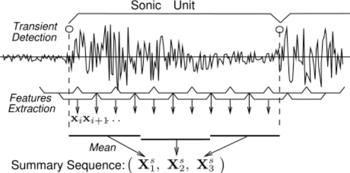
One of the advantages of the classifiers using alignment ker-nels is their ability to compare feature trajectories instead of isolated vectors. In order to exploit this ability, the choice of the segments to be compared has to be addressed. We believe that the feature trajectories are “meaningful” and distinctive of an instrument over the musical notes. How-ever, as the segmentation of an audio file into musical notes is a very complex task, we choose to perform an automatic segmentation into so-called sonic units. The sonic units are time segments which are supposed to be very close to musical notes.
We proceed as follows: First, silence frames are detected as in [5] and are removed from the data. Then an onset
2A source is a music recording such that different sources
constitute different recording conditions or different perform-ers/instrument instances.
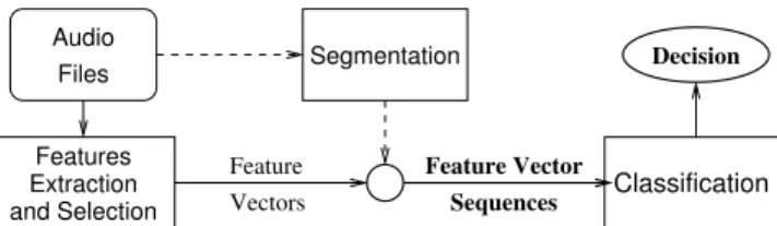
Files Audio Classification Segmentation Decision Features Extraction and Selection Feature Vectors Feature Vector Sequences
Figure 1: Principle of Sequences Classification
detector is run, using an algorithm proposed by Leveau and Daudet [7]. This algorithm detects transients, which are supposed to be note attacks. Finally, the sonic units are defined as the intervals between two successive onsets, as represented in Figure 2. In order to cope with the onset detector errors, the length of the sonic units is forced to be between 5 frames (0.1 s) and 125 frames (2 s), thus forbiding too short or too long segments.
The inputs of the classification systems are then the fea-ture vector sequences corresponding to these sonic units, as represented in Figure 1. Therefore, a classification decision is taken for each sonic unit.
3.2.3 Classification
The SVM classification software used for this study is based on the “SVM-Light” implementation by Joachims [6], which was extended in order to include the alignment kernels. The parameter C is set to 1, based on the results of previous work [5]. We test 9 values of the parameters σ2 for each kernel, between 0.25 and 32.
For the GMMs and HMMs, we use Murphy’s MATLAB tool-box [11]. We model the notes by a left-right 3-state HMMs, with an 8-component GMM in each state.
The training of the HMMs is performed with the EM algorithm over the separated sonic units. The states are supposed to capture respectively the attack, sustain and re-lease of each sonic unit. In order to have the same number of Gaussian components as for the HMM classifier, we tested a 24-component GMM system, but its performance was lower than a 8-component GMM. Therefore, we only present the results of the latter system.
The alignment kernels presented in Section 2.3 use a form of the DTW algorithm. The chosen weighting coefficients mπ(i) are equal to 1 for a “horizontal” or “vertical” step and
2 for a unitary “diagonal” step, so that the normalization coefficient Mπis independent of the alignment path.
Since in our database, the amount of data differs from one instrument to another, the score which we use to com-pare the classification systems is the average recognition rate, i.e. the average of all the classes recognition rates. With the figures (all expressed in percents), we also specify the radius of the largest 95% confidence interval (corresponding to the worst case), which will be referred to as confidence. 3.3 First Results
The results of our first experiments are given in Table 1. In these tests, we classify the feature vectors sequences corre-sponding to the sonic units, with 6 systems. The calculation of the SVM solutions using the alignment kernels Kξ and
Kχare not presented since the executions did not terminate
in acceptable running times. An explanation of this phe-nomenon may be the absence of normalization in the com-putation of these kernels (see Eq. 4). Consequently, the kernel values depend on the sequences length and the ob-tained gram matrix may be ill-conditioned, resulting in a bad convergence of the optimization algorithm.
We observe that the HMM system shows significantly better results than the GMM classifiers (+1.6% improvement
GMM+DF HMM 71.5 73.1 RBF-SVM+DF ξ-SVM+DF 76.2 75.9 GDTW-SVM DTAK-SVM 63.9 68.6
Table 1: Recognition Rates: Classification of Sonic Units. Confidence: 1%. We have chosen the best parameter σ for each SVM kernel: σ = 1 for the RBF kernel, σ = 2 for the kernel ξ and σ = 0.5 for the two alignment kernels.
whereas the 95% confidence interval radius is 1%), which suggests that taking into account the temporal dependency of the feature vectors does improve the classification perfor-mance. However, the “static” SVM systems perform better than both GMM and HMM classifiers. We believe that the reason lies in the fact that the latter classifiers are generative, assuming mixture of Gaussian densities which may not be appropriate for this problem, whereas SVMs are discrimina-tive classifiers that model the classes “boundaries” without supposing any special form of the probability densities.
However, we see that the SVM classifiers using the align-ment kernel GDTW and DTAK turn out to be ineffective. Indeed, they achieve the lowest classification scores among the systems we test. As these kernels appear not to be ap-propriate for our problem when used on feature vectors se-quences over the entire sonic units, we adopt another strat-egy where the classifiers are run on so-called summary se-quences.
3.4 Summary Sequences Classification
In this new approach, whose principle is represented in Fig-ure 2, the sonic units are split in a small number of subseg-ments of the same length. Then, the mean of the feature vectors is computed over each of the subsegments. Finally, the summary sequences (the sequences of these means), are classified so that a decision is made over every sonic unit. We run two sets of experiments, using 3 and 5 subsequences for each sonic unit. We choose these small numbers because the sonic units can be as short as 5-frames length.
Since the number of subsegments is constant, the length of these subsegments depends on the sonic unit total length. This choice may seem odd, as the summary sequence con-struction is in fact a kind of linear time-warping transfor-mation, which may interfere with the alignment algorithm embedded in the kernels. However, it is a way to overcome the normalization problem explained in Section 3.3 and thus use the kernels Kξand Kχ.
3 subsegments 5 subsegments GMM+DF 72.7 73.1 HMM 72.8 70.5 RBF-SVM+DF 76.7 75.5 ξ-SVM+DF 76.9 75.5 DTAK-SVM 75.2 73.7 GDTW-SVM 73.4 71.5 Kξ-SVM 77.8 76.5 Kχ-SVM 77.4 77.2
Table 2: Recognition Rates: Classification of Summary Se-quences. Confidence: 0.9%. In boldface are the best scores of the reference systems and of the alignment kernels.
The results of these experiments are presented in Ta-ble 2. The scores of the SVM classifiers are obtained with
Features Extraction Mean Sonic Detection Transient Summary Sequence: Unit . . . ` Xs 1, Xs2, Xs3 ´ xi+1 xi
Figure 2: Sonic unit segmentation and summary sequence. Here is represented a 3-subsegment summary sequence: the sonic unit is divided in 3 equal-length segments; the mean of the feature vectors xi is computed over each of the
subseg-ments; the summary sequence is then the sequence of these means (XS
1, XS2, XS3).
the best parameter σ2among those tested. We first observe
that the use of summary sequences achieves improved overall performance. Indeed, the scores of almost all the classifiers are higher than when considering every feature vector of the sonic units. The use of the means of the vectors over the sub-segments seem to attenuate the influence of the outliers, thus resulting in more robust decisions. This also explains why the systems show better performances with 3 subsegments than with 5.
We run the experiments using only one subsegment, thus classifying one isolated feature vector for each sonic unit. In this case, the alignment kernels are equivalent to the ref-erence “static” SVMs. The scores are lower than with 5 subsegments: the best recognition rate is 74.1%, obtained with the ξ-SVM system. The use of the features mean value alone does not improve the classification performance, which suggests that taking into account the sequential structure of the data is important.
However, additional tests using the kernels GDTW and DTAK with constant 3-frame and 5-frame subsegments (hence with a variable number of subsegments) show worse performances than with only one subsegment, although this transformation preserves more faithfully the sequential structure. This confirms that these kernels are not adapted to our problem.
For this classification of summary sequences, the clas-sifiers using the alignment kernel Kξ and Kχ achieve better
performances than the other classifiers. With 3 subsegments, the improvement is significant for the Kξ-SVM: its score is
77.8% average recognition rate whereas the best static sys-tem achieves 76.9%. These alignment kernels are also more efficient than the other classifiers when using 5 subsegments per sonic unit.
4. CONCLUSION
We have tested four examples of so-called alignment ker-nels, which allow one to use the powerful SVM classifiers on sequential data and to take into account the dependency be-tween the successive feature vectors. These kernels compute a similarity measure between two vectors sequences using a DTW-like alignment algorithm. We have compared their performances with other approaches for sequences classifi-cation in the music instrument recognition appliclassifi-cation. For two of these kernels, the results show an improvement of the recognition rates in comparison to the other classifiers when the systems are run on what we called summary sequences of sonic units. This indicates that alignment kernels are a promising approach which could be applied to other fields of
audio classification, allied with a well-chosen segmentation. The main drawback of the alignment kernels which have been found efficient is the complexity of the resulting SVMs. This prevents us from running them on whole sonic units sequences. Thus, a useful development would be to explore ways to overcome this increase of complexity, e.g. by a sub-sampling or by reducing the number of kernel evaluations. Another perspective for future work is the study of the in-fluence of the weighting coefficients mπ of the alignment
al-gorithm (see Section 2.3), as they are potentially important kernel parameters.
REFERENCES
[1] C. Bahlmann, B. Haasdonk, and H. Burkhardt. On-line handwriting recognition with support vector machines—a kernel approach. In Proc. of the 8th IWFHR, pages 49–54, 2002.
[2] M. Cuturi, J.-P. Vert, O. Birkenes, and T. Matsui. A kernel for time series based on global alignments. In IEEE International Conference on Acoustics, Speech and Signal Processing, pages 413–416. IEEE, April 2007. [3] R. Duda, P. Hart, and D. E. Stork. Pattern
Classifica-tion. Wiley-Interscience, 2001.
[4] A. Eronen. Musical instrument recognition using ica-based transform of features and discriminatively trained hmms. In 7th International Sumposium on Signal Pro-cessing and its Applications, 2003.
[5] S. Essid. Classification automatique des signaux audio-fr´equences : reconnaissance des instruments de musique. PhD thesis, ´Ecole Nationale Sup´erieure des T´el´ecommunications, Paris, 2005.
[6] T. Joachims. Svm-light toolbox. http://svmlight. joachims.org/.
[7] P. Leveau, L. Daudet, and G. Richard. Methodology and tools for the evaluation of automatic onset detection algorithms in music. In ISMIR, 2004.
[8] A. A. Livshin and X. Rodet. Musical instrument iden-tification in continuous recordings. In DAFX, 2004. [9] M. F. McKinney and J. Breebaart. Features for audio
and music classification. In International Symphosium on Music Information Retrieval, 2003.
[10] A. Meng. Temporal Feature Integration for Music Or-ganisation. PhD thesis, Technical University of Den-mark, DTU, 2006.
[11] K. Murphy. Hmm matlab toolbox. http://www.cs. ubc.ca/~murphyk/Software/HMM/hmm.html.
[12] G. Peeters. A large set of audio features for sound de-scription (similarity and classification) in the cuidado project. Technical report, IRCAM, 2004.
[13] J. Platt. Probabilistic outputs for support vector ma-chines and comparison to regularized likelihood meth-ods. In Advances in Large Margin Classifiers, 1999. [14] L. R. Rabiner. A tutorial on hidden markov models and
selected applications in speech recognition. Proceedings of the IEEE, 77(2):257–286, 1989.
[15] B. Scholkopf and A. J. Smola. Learning with Ker-nels: Support Vector Machines, Regularization, Opti-mization, and Beyond. MIT Press, Cambridge, MA, USA, 2001.
[16] H. Shimodaira, K. ichi Noma, M. Nakai, and S. Sagayama. Dynamic time-alignment kernel in sup-port vector machine. In NIPS 2002. MIT Press, 2002. [17] J.-P. Vert, H. Saigo, and T. Akutsu. Local alignment
kernels for biological sequences, pages 131–154. MIT Press, 2004.