HAL Id: hal-01407664
https://hal.archives-ouvertes.fr/hal-01407664
Submitted on 2 Dec 2016
HAL is a multi-disciplinary open access
archive for the deposit and dissemination of
sci-entific research documents, whether they are
pub-lished or not. The documents may come from
teaching and research institutions in France or
abroad, or from public or private research centers.
L’archive ouverte pluridisciplinaire HAL, est
destinée au dépôt et à la diffusion de documents
scientifiques de niveau recherche, publiés ou non,
émanant des établissements d’enseignement et de
recherche français ou étrangers, des laboratoires
publics ou privés.
Towards Visualizing Hidden Structures
Rémy Dautriche, Alexandre Termier, Renaud Blanch, Miguel Santana
To cite this version:
Rémy Dautriche, Alexandre Termier, Renaud Blanch, Miguel Santana. Towards Visualizing Hidden
Structures. International Conference on Data Mining (ICDM) / PhD Forum, 2016, Barcelone, Spain.
�hal-01407664�
Towards Visualizing Hidden Structures
R´emy Dautriche
∗‡, Alexandre Termier
†, Renaud Blanch
∗and Miguel Santana
‡∗University Grenoble Alps †University of Rennes 1 ‡STMicroelectronics
LIG IRISA F-38920 Crolles
F-38000 Grenoble F-35042 Rennes {surname.name}@st.com {surname.name}@imag.fr [email protected]
Abstract—There is an increasing need to quickly understand the contents log data. A wide range of patterns can be computed and provide valuable information: for example existence of repeated sequences of events or periodic behaviors. However pattern mining techniques often produce many patterns that have to be examined one by one, which is time consuming for experts. On the other hand, visualization techniques are easier to under-stand, but cannot provide the in-depth understanding provided by pattern mining approaches. Our contribution is to propose a novel visual analytics method that allows to immediately visualize hidden structures such as repeated sets/sequences and periodicity, allowing to quickly gain a deep understanding of the log.
I. INTRODUCTION
A large part of the huge volume of data available nowadays are logs of some real world or computer processes. A log is a sequence of timestamped events, where events are of arbitrary complexity but often share a similar structure, usually tuples of values or symbols. Such logs can hold valuable knowledge: for example analyzing a network log can show that an undesired intrusion took place and help to understand the intrusion method.
Possible analysis of computer logs can discover a repeated structure (main “regime”, disruptions of this main regime, or changes between stable regimes. Understanding what consti-tutes a regime is not trivial: it consists of some patterns of repetition in the events, and these patterns can, depending on the data and the use case, be of arbitrary complexity. They can be as simple as a mere repetition of a fixed set of events, or as complex as the respect of a complex sequencing of the events combined with periodicity constraints in the repetition. It would be of tremendous help to people analyzing logs to have a way to view “at a glance” how such structures exist over the trace, with the most prominent of those structures at each period of the trace as well their evolution over the trace. Existing methods for analyzing traces fall short to these expectations. Many methods are based on data visualization. They exploit various aggregation techniques to show the raw data of the trace in an understandable way while trying to minimize visual clutter. These methods do not explicitly show the structures described above. Depending on the level of abstraction chosen, some of these structure can be identified by the user’s eye. On the other end of the spectrum are data mining methods, more precisely pattern mining methods [1], [2]. These methods are designed to find repeated structures such as frequent itemsets, frequent sequences of various kinds, or periodic patterns. However, their output is served as a
(long) list, where results have to be examined one by one. Most visualization techniques for pattern mining results focus on the problem offering a navigational interface over the set of results, and we are not aware of any approach showing different patterns in context withing the data, allowing an “at a glance” understanding of complex structure evolution in the data.
The contribution of this paper is to propose a novel vi-sual analytics technique to understand at a glance the main structures existing in the data, as well as their evolution over time. This technique is designed for traces, and combines a data visualization approach with techniques inspired from pattern mining, but simplified for the purpose of making an understandable visualization.
Our experiment demonstrates the interest of our approach on a real use case: the execution trace of an embedded system and shows how.
The paper is organized as follows: Section II starts by exposing related work for visualizing the complex structures discovered by pattern mining methods. Then, Section III provides the main definitions necessary for the paper, and Section IV describes our algorithm to compute the strutures. Section V explains our structure visualization technique. The interest of our approach is demonstrated experimentally in Section VI, and Section VII concludes the paper and gives some perspectives.
II. RELATEDWORK
Many research have been done to propose visualization techniques for traces. Most of them focus on providing an overview of the whole trace using various aggregation tech-niques to mitigate the aliasing when rendering a large volume of data. Smart Traces uses multiple views that show different aggregation level [3]. Viva aggregates separately the event producers and the time axis and uses a treemap to visualize the results [4]. Refer to the survey on performance visualization tools for a complete review [5]. However, to our knowledge, there exists no techniques to visualize the structures in a trace to help the understanding of the main regime of the system and the potential perturbations.
There has been a long interest to provide visualization techniques helping to sift through the output of pattern mining algorithms. These are the closer work to our approach, we give below an overview of the existing work in this field.
The initial approach was based on using parallel coor-dinates [6], [7] to visualize association rules and frequent itemsets. An itemset with k items (a k-itemset) is represented with curves linking k vertical axis. The thickness of the links encodes the support of the itemset. The items are placed on vertical axis and ordered by groups. Items belonging to the same group are ordered according their frequency in the dataset. The number of vertical axis depends on the longest itemset to represent. The different items are linked together by lines that connect the vertical axis, thus, a line visually presents an itemset. The pre-ordering done on the axis aims to improve the readability of the representation by minimizing intersections between the lines. The main limitation using parallel coordinates is the lack of scalability. When many patterns need to be visualized, the visualization becomes too clutter with a large number of crossing lines making difficult the reading of a pattern.
CloseViz [8] adopts a different strategy. It visualizes only closed patterns with a single line and represents the items using a circle. It has the advantage of reducing significantly the amount of patterns to visualize. It is based on previous works FIsViz [9], WiFIsViz [10] and FpViz [11].
FIsViz [9] encodes the itemsets with polylines in a 2D rendering. The horizontal axis has k nodes for a k-itemset. The support of the items are encoded on the vertical axis. Similarly than with parallel coordinates, this technique quickly becomes tedious to read with many line crossing. WiFIsViz [10] and FpViz [11] aims to solve this issue by grouping the patterns us-ing common prefixes and horizontal lines instead of polylines. While the visualization benefits from these improvements, discovering relationships between the patterns and insightful information about the dataset remains a difficult task.
Other visualization techniques use a radial layout. FP-Viz [12] is a visualization tool for frequent itemsets. The items are placed on concentric circles and are represented by circular segments whose length encode its frequency. Therefore a k-itemset is rendered with k circular segments. The support of an itemset is encoded using a color-scale from green to red. When working with a large amount of itemsets, the information becomes tedious to read due to a high clutterness.
Bothorel et al. [13] proposed an other technique based on a circular layout, placing the itemset on concentric circles instead of items. The itemsets having the same cardinality are located on the same circle. The 1-itemset are disposed on the external cicle and the k-itemsets on the kth circle. Then, the frequent itemsets of each two neighbor circles are linked together. To improve the readability, an edge bundling algorithm is applied to simplify the graph between all the consecutive circles.
PowerSet viewer [14] is an other frequent itemset visu-alization tool. The screen space is divided into horizontal bands, one band contains the itemsets of a given cardinality, the 1-itemset being on the top. An itemset is represented by a rectangle and its frequency is encoded in the color. This technique allows to have an overview of the frequent itemsets in the data but lack representation of the support, and is limited
to a single type of pattern.
Note that there is a promising line of research in that field is to provide interactive interfaces for navigating the space of patterns, such as MIME from Goethals et al. [15]. Such work are not directly related to ours as they are designed around interactions with the user to explore a potentially huge space of patterns, while we focus on a smaller space of patterns but aim at an immediate understanding of the visualization.
All the previous work make the understanding of the individual items of the itemset a priority. They also rely on the complete set of frequent itemsets. Our approach is different: we consider patterns that are short (only 2 or 3 items, fixed length) but we put the focus on the different structures organizing these items: set, sequence, periodicity. Our visualization is built around this idea: the structures are the main information shown by the visualization, avoiding combinatorial explosion while showing valuable and usually unseen information.
III. DEFINITIONS ANDNOTATIONS
When analyzing logs or more generally time-oriented data, the goal is to understand the global and local trends inside the data and to find the outliers. A large panel of knowl-edge discovery and data mining (KDD) techniques focus on searching frequent patterns for meaningful information with no previous knowledge on the data. They return the results under the form of frequent patterns. Such patterns can be itemsets [16], periodic itemsets [1] or sequential patterns [17]. Depending on the nature of the pattern, the amount of in-formation conveyed vary. For instance, knowing the frequency of an itemset gives less information about the dataset than knowing the frequency of a sequence which itself convey less information than the frequency of a periodic sequence and so on. The more complex is the nature of a pattern, the more information is given to the analyst. Moreover, revealing how an itemset specializes into a sequence with the same items can also indicate relevant information or help filtering-out some parts of the dataset. In this section, we give basic definition in the context of mining logs and introduce the notion of structure.
A. Basic Definitions
Logs store a sequence of events. Each event has different properties depending on the nature of the logged system or application but common characteristics remain stable. All the events have a timestamp that corresponds to the moment when it has occurred. We note ts(e) the timestamp of the event e.
Each event has also a type, noted as et(e). We note the set of event types as T = {et0, et1, . . . , etn} and |T | is the
total number of event types in the data. For instance, in the case of web server logs, the event type can be the HTTP request whether it is a GET, POST, etc. When working with execution traces, the event type is the operation executed such as a context switch, an entry or exit of an interrupt or a system call.
We also consider that events are generated by “event pro-ducers” that we call actors. An actor is an entity that produces at least one event of the dataset. We note A = {a0, a1, . . . , an}
the set of actors producing at least one event in the dataset. When working with network logs, an actor can be an IP address. In the context of debugging embedded systems using execution traces, an actor is an interrupt, a process, a kernel module, etc. We note actor(e) the actor of the event e.
Our dataset D is a set of events contained in the log chrono-logically ordered {e0, e1, . . . , en}. Given an event e ∈ D,
its identifier id(e) is its position in the dataset. We have ∀ ei, ej∈ D, ts(ei) < ts(ej) if and only if id(ei) < id(ej).
The set of items I = T × A = {i0, i1, . . . , in} is the set of
all the event types in the data tagged by an actor. This ensures a finer-grained detailed patterns: it enables to differentiate an event type et produced by the actor ai from an event type
et produced by the actor aj (i.e a system call performed
by two different processes will be differentiated in the set of items). An item x occurs in the dataset D if and only if ∃ e ⊆ D, actor(e) ⊆ A, et(e) ⊆ T , et(e) × actor(e) = x.
An itemset, noted X = {x0, x1, . . . , xn} where xi is an
item i.e. xi ∈ I is an unordered set of items. A sequence,
noted S = hx0, x1, . . . , xni, where xi is an item i.e. xi ∈ I,
is an ordered set of items. A sequence S is a specialization of the itemset X if and only if ∀xi∈ S, xi∈ X.
A sequence S ⊆ X occurs in the dataset D if and only if ∀ xi, xj ∈ S, j − i = 1, ∃ em, en ∈ D, ts(em) <
ts(en), id(en) − id(em) = 1, et(em) × actor(em) =
xi, et(en) × actor(en) = xj. An itemset X occurs in the
dataset D if and only if there is at least one sequence S that occurs in D so that S is a specialization of X.
B. Structure
The most basic information computable for an itemset X is its frequency i.e. its number of occurrences in D. The support of an itemset X, noted supp(X), is the total number of occur-rences of its specialized sequences: supp(X) =P
isupp(Si),
with Si⊆ X and supp(Si) the number of occurrences of the
sequence Si in D.
A more sophisticated information about an itemset is the repartition of its specialized sequences. An itemset having k items, a k-itemset, contains k × k sequences of k items.
As an example, the sequences hA, Ai, hA, Bi, hB, Ai and hB, Bi are all specializations of the 2-itemset {A, B}.
We define as dominant the sequence S that has the highest support supp(S) among the specialized sequences of the itemset X. We note the dominant sequence of an itemset X as SX. This information is important to understand time-oriented
data: when considering a couple of events ei and ej, it is
insightful to know whether ei occurs before ej in most cases
or not. If not, none of these sequences brings more information about the data than the itemset {ei, ej}.
Knowing whether a sequence is periodic or not also brings meaningful insights about the log. Given a sequence S and a period p, we define (S, p) the set of consecutive occurrences of S separated by p items in the dataset. A sequence is periodic
if |(S, p)| is superior to a minimum threshold ρ. The coverage of a periodic sequence is defined as supp(S)|(S,p)| .
This provides information about whether S is very periodic or occurs mostly at irregular time intervals. Thus, for a given itemset X, we can compute the periodicity of each of its specialized sequences and determine what is the maximal periodicity among all the sequences of an itemsets, noted as pX.
With the combination of the support of an itemset, the repartition of its sequences with their periodicity, it becomes possible to find the sub-parts of the dataset that are mostly pe-riodic as well as whether the dataset contains mainly itemsets (no dominant sequences) or sequences.
We formalize this intuition with the concept of structure for an itemset. We define a structure as follows:
Definition 1. A structure is a quadruple (X, supp(X), SX, supp(SX), pX) with X ∈ X , SX the
dominant sequence of the itemset, supp(SX) the support of
SX and pX the maximal periodicity among the specialized
sequence of the itemset.
Note that in this paper we focus on the properties of itemset, sequence and periodicity, but other properties could easily be integrated in our tuple notation.
Let consider the following example:
hA, Bi hA, Bi {A, B} hB, Ai hB, Ai 25% 20% 80% 75%
In this example, the itemset X = {A, B} containing the items A and B is present in the dataset D respectively 20% and 80% of the time under the sequences hA, Bi and hB, Ai. The dominant sequence is SX = hB, Ai and its support is
supp(SX) = 0.8. The period p of each sequence as well
as a coverage of the sequences respecting this period has been computed. There is respectively 25% and 75% of the sequences hA, Bi and hB, Ai that are covered by the periods. The maximal periodicity of X is pX = 0.75. It gives a
structure noted ({A, B}, hB, Ai, 0.8, 0.75).
In this paper, we propose a novel interactive technique to visualize these structure, normally hidden to the users and show how it make apparent the underlying structures in the data such as periodic behaviors and perturbations.
IV. STRUCTURECOMPUTATION
In this section, we explain our algorithm to compute effi-ciently all the parameters of the structures. The goal of our tool is to show information usually hidden with the support of the structures. Therefore, it is important to keep the patterns as simple as possible and being able to quickly compute all the information necessary for the structures. Moreover, the computed results do not need to have an exact precision since they will serve as the input of a visualization. To fulfill these constraints, we designed an algorithm that computes the
patterns in a naive way but in a time short enough to be used in an interactive visualization.
Algorithm 1 Build structures
Input: Dataset D, itemset I, minimum sequence supportρ, number of time windows W
Output: all the structures that occur in the time windows of D
function BUILDSTRUCTURES(D, I, ρ, W ) structs ← [ ]
T W ←SLICEDATASET(D, W )
for all w ∈ T W do . in parallel for each w f reqItems ←BUILDFREQITEMS(w)
S ←BUILDSEQUENCES(f reqItems) seqOccs ←FINDSEQOCC(W, S) P ←FINDPERIOD(seqOccs)
structsw←BUILDSTRUCT(seqOccs, P, ρ)
ADD(structs, structsw)
return structs
The function SLICEDATASET splits the dataset D into W time windows. Slicing the dataset is an important parameter to set the precision of the results. It greatly influences the nature of the patterns discovered by the algorithms. When working with time-oriented data, the analysis becomes more local as the number of time windows to slice the time dimension increases. The task of the analyst may be to analyze globally the dataset to study the high-level properties of the structures. In this case, the dataset will be sliced in a few number of time windows. In contrary, comparing local behaviors can support the discovery of perturbations by detecting a different sets of structures in a time window. For each time slice, all the parameters of a structure described in section III are computed for all the possible itemsets. Doing this produces local results detailed for each time slice and makes possible to detect regular behavior across of the windows as well as perturbations that happened in a time slice. The structures are computed for each time window in parallel.
The function BUILDFREQITEMS compute the number of occurrences for each item xi ∈ I. It returns a set of items
f reqItems so that the occurrences of all the items x ∈ f reqItems covers 80% of the total number of the occurrences. By doing so, we are able to discard a large number of items that occur a few times and mitigates the computational time of the algorithm. Also, as the visualization aims to show the tendency inside the data, the sequences having a very low support are unlikely to be visible on the final rendering. Thus, discarding the least items that occur the least in the dataset prevent the sequences whose support supp(S) is very low.
The function BUILDSEQUENCES generates exhaustively all the possible sequences from the items contained in f reqItems. It returns a set S.
FINDSEQOCCfind all the occurrences for the sequences in f reqItems. This function is the most time consuming task of the algorithm so an efficient algorithm has to be used. We have implemented the SOG algorithm [18]. It is based on
bit parallelism and q-Grams to perform exact multiple pattern matching in linear time. In our case, the alphabet Σ is the set of items I, whose size |Σ| = |I| = |T × A|, can potentially be very large. The pattern to search in the dataset are the sequences for which we limit their size to be small. We have selected the SOG algorithm since it is the best performing algorithm for multiple pattern matching with a large alphabet size and a small pattern length [19]. We use 2-gram in our implementation: benchmark shows that using 3-gram is much slower and memory consuming than using 2-gram for up to 105 patterns.
The method FINDPERIOD takes as parameter all the posi-tions of the occurrences for each sequence. For each sequence, it performs a Fast Fourier Transform (FFT) and select the period p which allows to maximize |(S, p)|.
The final step, implemented in the functionBUILDSTRUCT
is to construct the structures from the results previously computed. It returns all the structures sorted according to support of the itemsets.
V. STRUCTUREVISUALIZATION
Visualizing the structures as defined in the previous section can reveal meaningful information about the underlying be-havior hidden in the data. According to Shneiderman [20], a good visualization technique has to provide a pipeline as Overview first, zoom and filter, then details-on-demand. When designing our technique, we followed this guideline and integrated an overview to visualize all the structures with a detailed representation of a single structure.
We begin by explaining which tasks the visualization tool has to support and what are the benefits it brings to leverage the difficulty of analyzing the structures. We continue with the description of the design of the visualization to render in a clear way a huge amount of structures, providing an overview of the dataset to understand the global trends and perturbations. The structure overview is coupled with a log overview, a stacked graph of the actors. Finally, we explain how a structure selected by the user is rendered in a detailed visualization. Figure 2 shows the whole interface with the different views described below.
A. Goals
In this work, we propose a visualization technique to enable the user to quickly understand the hidden structures in the data and designed to address the following goals:
1) Quickly understand the underlying structures contained in the dataset. Data mining algorithms provide a very large number of patterns in most cases. These results contain meaningful insights to support the understanding of the dataset. However, it is a very complex and time consuming task to take advantage of them and this task requires an expert. Providing an intuitive visualization technique is mandatory to harness the patterns and to shorten the time needed for the analysis.
2) Simplified parameters settings. Data mining techniques have different parameters to tune their output. The
visualization has to provide user interactions to simplify the exploration of the parameter space.
To better support the understanding of the structures, the visualization has to show the nature of the patterns whether it is an itemset, a sequential pattern and if it is periodic. For a given itemset, the information about the sequences repartition has also to be conveyed by the visual representation as well as if the sequences are periodic or not. Therefore, the visualization takes as input the support of the itemsets, the repartition of its sequences and the percentage of sequences covered by its period if any.
B. Log Overview
When analyzing logs, it is important to understand the repartition of the events across time. We chose to integrate a stacked graph, located at the top of the visualization, to represent the event density for the whole dataset (Figure 2a). The layers correspond to the actors of the log. To build the graph, we slice the trace into p time windows where p is the horizontal resolution in pixels of the screen space available. For each time window, we compute the event density of each actor and stack the values.
We chose a stacked graph [21] for its readability and for its capacity to convey two bits of information at any time of the trace: (1) the global number of events is visualized on the overall shape of the graph and (2) the thickness of a layer encodes the number of events an actor has produced at a specific time.
C. Structures Overview
The algorithm to compute the structures takes as parameter a number of time windows. Since the task cannot be pre-determined, this parameter is controlled interactively by the user at the moment of the analysis. By enabling this interac-tions, our tool supports the study of the evolution of behavioral patterns from a global to a local point of view.
1) Many Structures Visualization: To provide a clear vi-sualization that does not overwhelm the user by the amount of information, a structure has to be represented in a compact yet clear way. Let consider a structure S = (X, supp(X), SX, supp(SX), pX). The different components
of the structure are mapped on visual parameters. Figure 2a shows the structures visualized below the log overview.
A structure S is represented with a rectangle whose support supp(X) is encoded in the height of the rectangle. The vertical space is completely filled with all the itemset. Its width is constrained by the size of the time slice. In each time window, the structures are ranked according to the support supp(X): the greater its support, the higher its position. By doing so, more visual space is given for the most frequent itemsets which are concentrated at the top of the rendering. It ensures that the most active actors are quickly detected by the eye.
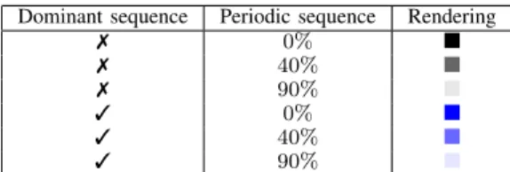
Next, the color encodes the information indicating whether an itemset has a dominant sequence or not. We define a thresh-old ρ to determine if the itemset has a dominant sequence. If ρ ≤ supp(SX), the itemset X has a dominant sequence. In this
Dominant sequence Periodic sequence Rendering
7 0% 7 40% 7 90% 3 0% 3 40% 3 90%
TABLE I: Visual representations of a structure
Fig. 1: Visualization of a structure. Each branch corresponds to one of its specialized sequence SX that occurs at least once
in the dataset. The thickness of the first and second segments respectively encode supp(SX) and pX. The branch colored in
red represents the sequence currently highlighted by the user while exploring the data. On the top left are rendered all the items belonging to the itemset of the structure.
case, the rectangle is rendered in blue otherwise, the rectangle of the itemset is filled with black. Areas of the logs where the data are more structured can be quickly spotted.
Lastly, we encode in the channel alpha (i.e. in the opacity) of the rectangle the periodicity of the sequence SX, pX.
The more a sequence is periodic, the more transparent is the rectangle representing the structure. When working with dataset where the structures are mostly periodic, it is important to fade out the periodic data since it corresponds to the correct behavior. Table I shows different rendering of an itemset depending on the value of the parameters.
When hovering a structure, all the rectangles representing SX become red (Figures 2b, 3) as well as the layer of the
actors present in the sequence. This shows the distribution of a single sequence over the whole dataset. A visualization of the structure also appears next to the cursor to show a detailed representation of the itemset, its sequences and periodicity. D. Visualizing Structure Details
Following the Shneiderman’s guidelines, more details can shown when requested by the user. When hovering a structure, a tooltip appears representing all the values of the structures. On the overview, to better make apparent the regular behavioral patterns, partial information about the itemsets and their specialized sequences are shown, hiding important information: how an itemset specializes into its sequences and what are precisely the items.
The tooltip shows these information using a Sankey diagram (Figure 1). Traditionally used to represent flow of energy and resources, it encodes here the differ-ent parameters of a structure. The figure represdiffer-ents the structure (X = {C@2401, E@2401, C@Idle}, SX =
hC@Idle, C@2401, E@2401i, supp(SX) = 0.53, pX =
0.46).
On the top left of the tooltip, the items of X are listed next to a square filled with the color of the actor used in the log overview. The root of the diagram (on the left) is the itemset X of the structure, in black to be consistent within the different views as an itemset with no dominant sequence is rendered in black. The itemset split into different branches, one branch per specialized sequence of the itemset that has at least one occurrence in the dataset. The branch are colored according to the user defined threshold ρ that set the minimum coverage of a periodic sequence and their thickness encodes the support of the sequence. The branch corresponding to the highlighted structure is colored in red. At the end of each branch, the sequence is represented using one square per item. Each square is filled with the actor’s color of the item and the event type is written on the square.
On Figure 1, the highlighted branch is half the height of the itemset since supp(SX) = 0.5.
The last segment of the branches corresponds to pX. The
wider the last segment, the higher pX. It shows intuitively to
the user how periodic the sequences are. In our example, we have pX = 0.46, thus the last segment is 0.46× as wide as
the previous segment.
VI. EXPERIMENT
In this section, we present a use case with execution traces for embedded systems. We begin by describing the input data, what are the events, the event producers, the actors and how we built the dataset D. The experiment shows that visualizing structures can efficiently reveal structural behavior and perturbations quickly.
The data are traces recorded during the execution of a streaming multimedia applications used to play music and video.
Multimedia applications receive the video and/or the music as an encoded stream. They have to decode it in real-time and send it to one or several output such as a television or speakers. In order to provide a smooth playback to the end user (i.e. no video artifacts or audio glitches), the decoding process has to respect some QoS properties [22]. Typically, when playing a movie, the decoding application has to output 25 frames per second. Under these conditions, traditional debuggers are irrelevant since using breakpoints pauses the execution and breaks the real-time constraints. Instead, the typical debugging method in this context is to record a trace during the execution of the application and analyze it post-mortem. There exists different tools to record execution traces such as KProbes that comes natively with the Linux kernel [23] or commercial solutions like KPTrace developed by STMicroelectronics [24]. Execution traces basically store all the events that occurred during the execution of an application on a system. It stores low-level events such as entry and exit of interrupts, events that occurred at the operating system level such as the system calls and the context switches and the entry and exit of the user applications. The dataset D contains all the events that
occurred during the execution. The set of actors A are the processes and interrupts that produced at least one event during the execution, noted with their process id (PID) in the tool. The event types T are the instructions executed. It can be a context switch (C), an entry (E) or exit (X) of a system call, an entry or exit of an interrupt respectively noted as I and i in the visualization. Examples of items contained in the set of items I = A × T are C@1234 (a context switch on process 1234), E@4321 (a system call performed by the process 4321) and i@Interrupt 567 (exit of the interrupt 567). In this usecase, we show how understanding the structures in the data supports the developers to debug their application.
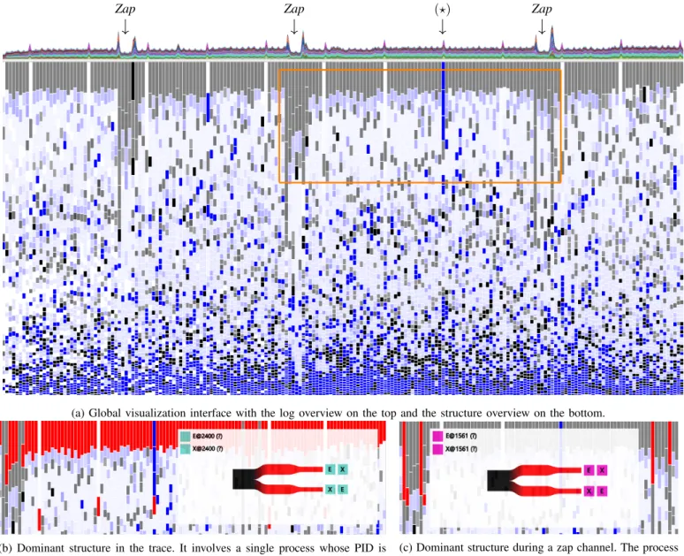
The stacked graph at the top represents the event density for each of these producers, hence a peak on the graph shows a local increase of the number of events on the system. In this use case, the execution trace has been recorded on an embedded system that decodes a multimedia stream for the television. The stream is received through the network on the Ethernet port.
During the execution, the user has changed three times the channel to decode (channel zap). These moments correspond to the three peaks of activity that appear on the stacked graph (see the log overview on Figure 2).
On the structure overview (Figure 2), three horizontal areas appear: a gray area on the top, a clear middle section and a mostly blue area at the bottom. The top grey bar shows that the most frequent structure on the whole trace is a structure that has no dominant sequence and limited periodicity. It involves a single process (the process 2400) that performs a huge amount of system calls (Figure 2b). The itemset has no dominant sequence due to its small size (2 items) and a high frequency. Its behavior is disturbed when a zap occurs: there is a much higher number of frequent itemset involving different processes. The structures show that during a zap, a single process mostly works, performing many system calls (Figure 2c). No periodic sequence appears: this reflects the perturbation of periodic decoding behavior when switching the stream to decode.
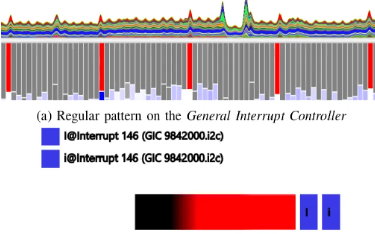
A very periodic sequence occurs regularly among the most frequent structures and appear as white bands on Figure 2, highlighted on Figure 3a. It shows a behavioral pattern at a lower frequency involving an interrupt named GIC, namely General Interrupt Controller(Figure 3). It consists in a general hardware resource to manage the interrupts.
The visualization shows a periodic sequence: it consists in the entry and the exit of the interrupt and shows a periodicity breaking by a blue bar (noted as (?) on Figure 2a). It shows the developer that an abnormal behavior happened in this time window.
The middle section contains a large amount of periodic structures. This is induced by the nature of the application: decoding a multimedia stream is a very periodic task: frames are decoded at a constrained rate (typically 25 frames per second) to ensure a smooth video playback. On the bottom we have many sequences. This is a normal behavior since the functions are called sporadically, generating many entry/exit
Zap Zap (?) Zap
(a) Global visualization interface with the log overview on the top and the structure overview on the bottom.
(b) Dominant structure in the trace. It involves a single process whose PID is 2400 that performs a huge number of system calls.
(c) Dominant structure during a zap channel. The process 1561 performs many system calls.
Fig. 2: Structures of an execution trace. The orange rectangle on Figure 2a corresponds to the area for Figure 2b and Figure 2c. events in the trace.
VII. CONCLUSION
We have presented a novel visual analytic technique that shows the hidden structures in logs. It enables the analysts of such logs to understand “at a glance” the repetitive behaviors that can be complex patterns involving sequences of events and periodicity, depending on the nature of the data. The regular behavior that implies repetitive structures are easily detected as well as the perturbations over the trace. Through an experiment, we have shown the relevance of our technique for the analysis of execution traces, proving our approach can be applied with a broader type of data than computer logs.
Our work opens several perspectives. A direct perspective is to improve the performances of the computation algorithm for the structures to achieve an interactive response time (up to 10ms). The core of our algorithm is the multiple pattern matching SOG algorithm. Existing work has described
a solution to implement it on GPU to reduce significantly the computation time [25].
Other perspectives consist in investigating visualization techniques of more complex structures. In this work, we have used the itemsets, sequences and periodic sequences as patterns. An other type of data structure can include a graph for the study of structures in logs of dynamic graphs. For instance, this could be used to visualize the evolution of structures in social graphs such as Twitter or Facebook. The main challenge relies in the mapping of a larger number of parameters of a structure onto visual attributes while having an uncluttered rendering to keep visualizing such structure “at a glance”.
REFERENCES
[1] P. L´opez Cueva, A. Bertaux, A. Termier, and J.-F. M´ehaut, “Debug-ging embedded multimedia application traces through periodic pattern mining,” in Proceedings of the 10th ACM Internation Conference on Embedded Software, 2012, pp. 13–22.
(a) Regular pattern on the General Interrupt Controller
(b) Visualization of the structure corresponding to the inter-rupt 146. The structure is composed of only one sequence hI@Interrupt146, i@Interrupt146i, that stands for entry and then exit of interrupt 146. The sequence is very periodic.
Fig. 3: Periodic behavior of the interrupt 146 shown on the structure overview and in details.
[2] S. Lagraa, A. Termier, and F. P´etrot, “Scalability bottlenecks discovery in mpsoc platforms using data mining on simulation traces,” in Design, Automation & Test in Europe Conference & Exhibition, DATE 2014, Dresden, Germany, March 24-28, 2014, 2014, pp. 1–6. [Online]. Available: http://dx.doi.org/10.7873/DATE.2014.199
[3] D. K. Osmari, H. T. Vo, C. T. Silva, J. L. D. Comba, and L. Lins, “Visu-alization and analysis of parallel dataflow execution with smart traces,” in 27th Conference on Graphics, Patterns and Images (SIBGRAPI), 2014.
[4] R. Lamarche-Perrin, L. M. Schnorr, and J.-M. Vincent, “Evaluating trace aggregation for performance visualization of large distributed systems,” in Proceedings of the 2014 IEEE Internation Symposium on Performance Analysis of Systems and Software, 2014.
[5] K. E. Isaacs, A. Gim´enez, A. Bhatele, M. Schulz, B. Hamann, and P. T. Bremer, “State of the art of performance visualization,” 2014. [6] L. Yang, “Visualizing frequent itemsets, association rules, and sequential
patterns in parallel coordinates,” in Computational Science and Its Applications - ICCSA 2003, 2003, pp. 21–30.
[7] ——, “Pruning and visualizing generalized association rules in parallel coordinates,” IEEE Transactions on Knowledge and Data Engineering, vol. 17, pp. 60–70, 2005.
[8] C. L. Carmichael and C. K.-S. Leung, “Closeviz: Visualizing useful patterns,” in Proceedings of the ACM SIGKDD Workshop on Useful Patterns, 2010, pp. 17–26.
[9] C. K.-S. Leung, P. P. Irani, and C. L. Carmichael, “Fisviz: A frequent itemset visualizer,” in Advances in Knowledge Discovery and Data Mining, 2008, pp. 644–652.
[10] ——, “Wifisviz: Effective visualization of frequent itemset,” in 2008 8th IEEE Conference on Data Mining, 2008, pp. 875–880.
[11] C. K.-S. Leung and C. L. Carmichael, “Fpviz: A visualizer for fre-quent pattern mining,” in Proceedings of the ACM SIGKDD Workshop on Visual Analytics and Knowledge Discovery: Integrating Automated Analysis with Interactive Exploration, 2009, pp. 30–39.
[12] D. A. Keim, J. Schneidewind, and M. Sips, “Fp-viz: Visual frequent pattern mining,” in IEEE Symposium on Information Visualization (InfoVis 05), 2008, Poster Paper.
[13] G. Bothorel, M. Serrurier, and C. Hurter, “Visualization of frequent item-sets with nested circular layout and bundling algorithm,” in Advances in Visual Computing -9thInternational Symposium, 2013, pp. 396–405.
[14] T. Munzner, Q. Kong, R. T. Ng, J. Lee, J. Klawe, D. Radulovic, and C. K. Leung, “Visual mining of power sets with large alphabets.” Department of Computer Science, The University of British Columbia, Vancouver, BC, Canada, 2005, Technical Report TR-2005-25.
[15] B. Goethals, S. Moens, and J. Vreeken, “MIME: a framework for interactive visual pattern mining,” in Proceedings of the 17th ACM SIGKDD International Conference on Knowledge Discovery and Data Mining, San Diego, CA, USA, August 21-24, 2011, 2011, pp. 757–760. [Online]. Available: http://doi.acm.org/10.1145/2020408.2020529
[16] J. Cheng, Y. Ke, and W. Ng, “A survey on algorithms for mining frequent itemsets over data streams,” Knowledge of Information Systems, vol. 16, pp. 1–27, 2008.
[17] C. H. Mooney and J. F. Roddick, “Sequential pattern mining – ap-proaches and algorithms,” ACM Computer Survey, vol. 45, pp. 19:1– 19:39, 2013.
[18] L. Salmela, J. Tarhio, and J. Kytojoki, “Multi-pattern matching with q-grams,” Journal of Experimental Algorithmics, vol. 11, pp. 1–19, 2006. [19] C. S. Kouzinopoulos and K. G. Margaritis, “Multiple pattern match-ing: Survey and experimental results,” Neural, Parallel, and Scientific Computation, vol. 22, pp. 563–593, 2014.
[20] B. Shneiderman, “The eyes have it: A task by data type taxonomy for information visualization,” in Visual Languages, 1996. Proceedings., IEEE Symposium on, 1996, pp. 336–343.
[21] L. Byron and M. Wattenberg, “Stacked graphs: Geometry & aesthetics,” IEEE Transactions on Visualization and Computer Graphics, vol. 14, pp. 1245–1252, 2008.
[22] O. Iegorov, V. Leroy, A. Termier, J.-F. Mehaut, and M. Santana, “Data mining approach to temporal debugging of embedded streaming applications,” in 2015 International Conference on Embedded Software (EMSOFT), 2015, pp. 167–176.
[23] R. Krishnakumar, “Kernel korer: Kprobes - a kernel debugger,” Linux Journal, vol. 2005, no. 133, 2005.
[24] C. Prada-Rojas, F. Riss, X. Raynaud, S. De Paoli, and M. Santana, “Observation tools for debugging and performance analysis of embedded linux applications,” in Conference on System Software, SoC and Silicon Debug-S4D, 2009.
[25] C. S. Kouzinopoulos, P. D. Michailidis, and K. G. Margaritis, “Multiple string matching on a gpu using cuda,” Scalable Computing: Practice and Experience, vol. 16, no. 2, pp. 121–137, 2015.