HAL Id: hal-00648681
https://hal.inria.fr/hal-00648681
Submitted on 6 Dec 2011
HAL is a multi-disciplinary open access
archive for the deposit and dissemination of
sci-entific research documents, whether they are
pub-lished or not. The documents may come from
teaching and research institutions in France or
abroad, or from public or private research centers.
L’archive ouverte pluridisciplinaire HAL, est
destinée au dépôt et à la diffusion de documents
scientifiques de niveau recherche, publiés ou non,
émanant des établissements d’enseignement et de
recherche français ou étrangers, des laboratoires
publics ou privés.
Moutarde
To cite this version:
Cyril Furtlehner, Yufei Han, Jean-Marc Lasgouttes, Victorin Martin, Fabien Moutarde. Propagation of
information on undirected dependency graphs for road traffic inference. CCT’11 - Chaos, Complexity
and Transport, May 2011, Marseille, France. �hal-00648681�
Propagation of information on undirected dependency graphs
for road traffic inference
Cyril Furtlehner∗ Yufei Han†Jean-Marc Lasgouttes‡
Victorin Martin‡Fabien Moutarde†
∗ INRIA Saclay LRI, France
† ROBOTIC Lab, Mines Paris-Tech France
‡INRIA Paris-Rocquencourt,France
In this paper we will review some properties of the “belief propagation” iter-ative map used to perform Bayesian inference in a distributed way. We use this algorithm as a starting point to address the inverse problem of encoding observation data into a probabilistic model. and focus on the situation when the data have many different statistical components, representing a variety of independent patterns. Asymptotic analysis reveals a connection with some Hopfield model. We then discuss the relevance of these results to the problem of reconstructing and predicting traffic states based on floating car data and show some experiments based on artificial and real data.
1. Introduction
The "belief propagation algorithm", originated in the artificial intelligence
com-munity for inference problems on Bayesian networks.16 It is a non-linear
iter-ative map which propagates information on a dependency graph of variables in the form of messages between variables. It has been recognised to be a generic procedure, instantiated in various domains like error correcting codes, signal processing or constraints satisfaction problems with various names
de-pending on the context:11the forward-backward algorithm for Hidden Markov
Model selection; the Viterbi algorithm; Gallager’s sum-product algorithm in Information theory. It has also a nice statistical physics interpretation, as a
minimiser of a Bethe free energy22or as a solver of TAP equations in the
spin-glass context.10As a noticeable development in the recent years, related to the
connection with statistical physics is the emergence of a new generation of algo-rithms for solving difficult combinatorial problems, like the survey propagation
algorithm13for constraint satisfaction problems or the affinity propagation for
clustering.3
The use we make of this algorithm in this work is twofold. Assuming a set of high dimensional data, in the form of sparse observations covering a finite fraction of segments in a traffic network, we wish to encode the dependencies
between the variables in a MRF in such a way that inference on this MRF with BP is optimal in some way. The paper is organised as follows: in Section 2 we introduce the BP algorithm and review some of its properties. In Section 3 we describe the traffic application and the inference model. In Section 4 we give a statistical physics analysis of this model. Finally in Section 5 we present some preliminary tests of the method.
2. The Belief Propagation Algorithm
We consider a set of discrete random variables x = {xi, i ∈ V} ∈
{1, . . . , q}|V |obeying a joint probability distribution of the form
P(x) = Y a∈F ψa(xa) Y i∈V φi(xi), (1)
where φi and ψa are factors associated respectively to a single variable xi
and to a subset a ∈ F of variables, F representing a set of cliques. The
ψaare called the “factors” while the φiare there by convenience and could be
reabsorbed in the definition of the factors. This distribution can be conveniently
graphically represented with a bi-bipartite graph, called the factor graph;11
F together with V define the factor graph G, which will be assumed to be connected. The set E of edges contains all the couples (a, i) ∈ F × V such
that i ∈ a. We denote da (resp. di) the degree of the factor node a (resp.
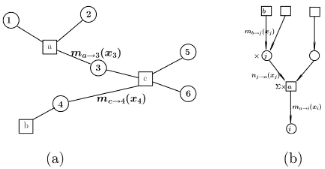
to the variable node i). The factor graph on the Figure 2.1.a corresponds for example to the following measure
p(x1, . . . , x6) = 1
Zψa(x1, x2, x3)ψb(x4)ψc(x3, x4, x5, x6)
with the following factor nodes a = {1, 2, 3}, b = {4} and c = {3, 5, 6}.
a b c 1 2 3 4 6 5 mc→4(x4) ma→3(x3) b i j a ma→i(xi) nj→a(xj) × Σ mb→j(xj) ×
(a)
(b)
Fig. 2.1. Example of factor graph (a) and message propagation rules (b).
Assuming that the factor graph is a tree, computing the set of marginal
dis-tributions, called the belief b(xi = x) associated to each variable i can be
done efficiently. The BP algorithm does this effectively for all variables in one single procedure, by remarking that the computation of each of these marginals
involves intermediates quantities called the messages ma→i(xi) [resp. ni→a]
“sent” by factor node a to variable node i [resp. variable node i to factor node a], and which are necessary to compute other marginals. The idea of BP is
to compute at once all these messages using the relation among them as a fixed point equation. Iterating the following message update rules sketched on Figure 2.1.b: 8 > > < > > : ma→i(xi) ← X xa\xi Y j ∈a/i nj →a(xj)ψa(xa) ni→a(xi) ← φi(xi) Y b∋i mb→i(xi)
yields, when a fixed point is reached, the following result for the beliefs,
b(xi) = 1 Zi φi(xi) Y a∋i ma→i(xi) b(xa) = 1 Za ψa(Xa) Y i∈a ni→a(xi).
This is exact if the factor graph is a tree and only approximate on multiply con-nected factor graphs. As mentioned before, the set of beliefs which is obtained
corresponds to a a stationary point of a variational problem.22Indeed, consider
the Kullback-Leibler divergence between a test joint distribution b(x) with the reference one p(x). The Bethe approximation yield the following functional of
the beliefs, including the joint beliefs ba(xa) corresponding to each factor:
DK L(b, p) = X {x} b({x}) log b({x}) p({x}) ≃ X a,xa ba(xa) log ba(xa) Q i∈abi(xi)ψ(xa)+ X i,xi logbi(xi) φi(xi) def = FB ethe= E − SB ethe
This is equivalent to say that we look for a minimiser of DK L(b, p) in the
following class of joint probabilities:
b(x) = 1 Z Y a ba(xa) Q i∈abi(xi) Y i bi(xi)
under the constraint that X
xa\xi
ba(xa) = bi(xi) ∀a ∈ F, ∀i ∈ a.
For a multi-connected factor graph, the beliefs are then interpreted as pseudo-marginal distribution, it is only when G is simply connected that these are genuine marginal probabilities of the reference distribution p.
There are a few properties of BP that are worth mentioning at this point. At first BP is a fast converging algorithm:
• Two sweeps over all edges are needed if the factor-graph is a tree.
• The complexity scales heuristically like KN log(N) on a sparse factor-graph with connectivity K.
However, when the graph is multiply connected, there is little guarantee on the
convergence15even so in practice it works well for sufficiently sparse graphs.
Another limit in this case, is that the fixed point may not correspond to a true measure, so in this sense the obtained beliefs albeit compatible among each other are considered only as pseudo-marginals. Finally for such graphs the uniqueness of fixed points is not guaranteed, but what has been shown is that:
• stable BP fixed points are local minima of the Bethe free energy;8
• the converse is not necessarily true.18
There are two important special cases, where the BP equations simplify:
(i) For binary variables: xi ∈ {0, 1}. Upon normalisation the messages are
parametrised as:
ma→i(xi) = ma→ixi+ (1 − ma→i)(1 − xi),
which is stable w.r.t. the message update rule. Then the propagation of
infor-mation reduces to the scalar quantity ma→i.
(ii) For Gaussian variables, the factors are necessarily pairwise, of the form
ψij(xi, xj) = exp n −1 2[xixj]Aij »xi xj – o φi(xi) = exp˘hixi¯.
Since factors are pairwise, messages can then be considered to be sent directly from one variable node i to another j with a Gaussian form:
mi→j(xj) = exp`−
(xj− xij)2
2σij
´.
This expression is also stable w.r.t. the message update rules. Information is
then propagated via the 2-component real vector (xij, σij) with the following
update rules: xij ←− 1 Aij X k∈i\j xik σik + hi, σij ←− 1 A2 ij ˆAii+ X k∈i\j 1 σik ˜.
In this case there is only one fixed point even on a loopy graph, not necessarily stable, but if convergence occurs the single variables beliefs provide the exact
marginals.19In fact for continuous variables, the Gaussian distribution is the
only one compatible with the BP rules. Expectation propagation14is a way to
address more general distributions in an approximate manner.
3. Application context
3.1. Problem at hand
Once the underlying joint probability measure is given this algorithm can be very efficient for inferring hidden variables, but in real application it is often the case that we have first to build the model. This is precisely the case for the
application that we are considering concerning the reconstruction and predic-tion of road traffic condipredic-tions, typically on the secondary network from sparse observations. Existing solutions for traffic information are classically based on data coming from static sensors (magnetic loops) on main road axis. These devices are far too expensive to be installed everywhere in all streets on the traffic network and other sources of data have to be found. One recent solution comes from an increasing number of vehicles equipped with GPS and able to exchange data through cellular phone connections for example, able therefore to produce so-called Floating Car Data (FCD). Our objective in this context is to build an inference schema adapted to these FCD, able to run in real time
and adapted to large scales road network, of size ranging from 103to 105in
the number of segments. In this respect, the BP algorithm seems well suited, but the difficulty is to construct a model based on these FCD.
3.2. Statistical modelling and Inference schema
To set the inference schema, we assume that a large amount of FCD sent by probe vehicles concerning some area of interest are continuously collected over a reasonable period of time (one year or more) such as to allow a finite fraction (a few percents) of road segments to be covered in real time. Our approach is defined as follows:
• Historical FCD are used to compute empirical dependencies between contigu-ous segments of the road network.
• These dependencies are encoded into a graphical model which vertices are (segment,timestamps) pairs attached with a congestion state, i.e. typically congested/not-congested.
• Congestion probabilities of the various unvisited segments or in the short-term future are computed with BP, conditionally to real-time data.
On the factor-graph the information is propagated both temporally and spa-tially. In this perspective, reconstruction and prediction are taken on the same footing, even so we expect of course future prediction to be less precise than reconstruction.
This schema is based on a statistical description of traffic data which is obtained by spatial and temporal discretization, in terms of road segments i and discrete time slots t corresponding to time windows of typically a few min-utes, leading to consider a set of vertices V = {α = (i, t)}. At each vertex
is attached a microscopic degree of freedom xα∈ E being a descriptor of the
corresponding segment state like for example, E = {0, 1}, 0 for congested and 1 for fluid. The model itself is based on historical data in form of
em-pirical marginal distributions ˆp(xα), ˆp(xα, xβ) giving reference states and
statistical interactions between degrees of freedom. Finally reconstruction and prediction is produced in the form of conditional marginal probability
distri-bution p(xα|V∗) of hidden variables V\V∗conditionally to the actual state
of variables in the set V∗= of observed variables.
In addition to this microscopic view, it is highly desirable to enrich the de-scription with macroscopic variables able in particular to capture and encode the temporal dynamics of the global system. These can be obtained by some linear analysis, e.g. PCA or with non-linear methods of clustering providing possibly hierarchical structures. Once some relevant variables are identified, we
can expect to have both a macroscopic description of the systems which can potentially be easily coupled to the microscopic one, by adding some nodes into the factor-graph. These additional degrees of freedom would be possibly interpreted in terms of global traffic indexes, associated to regions or compo-nents.
3.3. MRF model and pseudo moment matching calibration
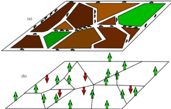
At the microscopic level the next step is to define a MRF, on which to run BP with good inference properties. For the rest of the paper, we consider a
binary encoding xi,t∈ {0, 1}, which we interpret as congested/not-congested
latent state, such that the MRF will actually be an Ising model as illustrated on Figure 3.1. We have to answer the two related questions:
• Given the historical data p(xˆ i,t), ˆp(xi,t, xj,t′) which joint law
P ({xi,t, (i, t) ∈ V})?
• Given new observation {x∗
i,t, (i, t) ∈ V∗} how to infer {xi,t, (i, t) ∈
V\V∗}?
(a)
(b)
Fig. 3.1. Underlying Ising modelling of traffic configurations.
The solution that we have been exploring5 are based on mean-field techniques
in statistical physics. It consists to use the Bethe approximation for the encod-ing and the belief-propagation for the decodencod-ing, such that the calibration of the model is coherent with the inference algorithm. In particular, when there is no real time observation, the reference point is given by the set of historical belief, so we want that running BP on our MRF delivers precisely these beliefs. Stated differently, we look for the φ and ψ defining the MRF in (1) such that the beliefs match the historical marginals:
ba(xa) = ˆpa(xa)
There is an explicit solution to this problem, because BP is know to be coherent
with the Bethe approximation,22a consequence of what is that any BP fixed
point b has to verify
P(x) = Y i∈V φi(xi) Y a∈F ψa(xa) = Y i∈V bi(xi) Y a∈F ba(xa) Q i∈abi(xi) . (2)
A sa result, a canonical choice for the functions φ and ψ is simply
φi(xi) = ˆpi(xi), ψa(xa) = Qpˆa(xa)
i∈apˆi(xi)
(3)
going along with ma→i(xi) ≡ 1 as a particular BP fixed point. In
addi-tion, from the reparametrization property of BP,17any other choices verifying
(2) produces the same set of fixed points with the same convergence proper-ties. Note that more advanced methods than the Bethe Approximation have been proposed, corresponding mainly to various levels of accuracy in the linear
response theory, for matching pseudo-moments12,20,21but at a higher
compu-tational price.
Next, for the decoding part, inserting information in real time in the model is done as follows. In practice observation are in the form of real numbers like speed or travel time. One possibility is to project such an observation onto the
binary state xi= 0 or xi= 1 but in practice this proves to be too crude. Since
the output of BP is anyway in the form of beliefs, i.e. real numbers in [0, 1], the idea is to exploit the full information by defining a correspondence between
observations Yi and probabilities p∗(xi = 1). The optimal way of inserting
this quantity into the BP equations,4 is obtained variationally by imposing
the additional constraint bi = p∗(xi) which results in modified messages sent
from i ∈ V∗, now reading
ni→a(xi) = p∗ i(xi) ma→i(xi) " = p ∗ i(xi) bi(xi) Y a′∋i,a′6=a ma′→i(xi) #
4. Statistical Physics Analysis
Some preliminary experiments of this procedure performed in5 indicate that
many BP fixed point can exist in absence of information, each one
correspond-ing to some congestion pattern like e.g. congestion/free flow. In6we have
anal-ysed the presence of multiple fixed points by looking at a study case and we outline some of the results in this section. In this study we considered a gen-erative hidden model of traffic in the form of a probabilistic mixture, C ≪ N being the number of mixture components, with each component having a sim-ple product form:
Phidden(x) def = 1 C C X c=1 Y i∈V pci(xi). (4)
The interpretation of this model is that traffic congestion is organised in var-ious patterns which can show up at different moments. We then studied the behaviour of our inference model on the data generated by this hidden proba-bility by adding a single parameter α into its definition (3):
φi(xi) = ˆpi(xi), ψij(xi, xj) =
“ pˆij(xi, xj)
ˆ
pi(xi) ˆpj(xj)
”α
where ˆpiand ˆpij are again the 1− and 2− variables frequency statistics that
constitute the input of the model while (4) is assumed to be unknown. In addition we impose some sparsity in the factor graph with help of some se-lection procedure of the links to maintained a reduced mean connectivity K. The typical numerical experiment we perform, given a configuration randomly
sampled from (4), is to reveal gradually the variables xV∗ in a random order
and compute conditional predictions for the remaining unknown variables. We then compare the beliefs obtained with the true conditional marginal
proba-bilities P (xi = x|xV∗) computed with (4), using an error measure based on
the Kullback-Leibler distance:
DKL def =D X x∈{0,1} bi(x) log bi(x) P (xi= x|xV∗) E V∗.
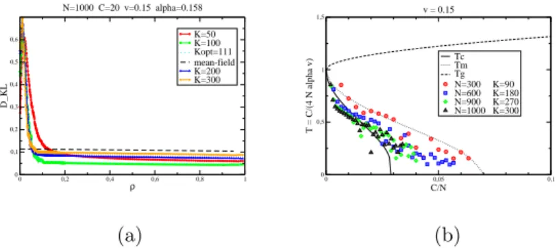
A sample test shown on Figure 4.1.a indicates for example that on a system
0 0,2 0,4 0,6 0,8 1 ρ 0 0,1 0,2 0,3 0,4 0,5 0,6 D_KL K=50 K=100 Kopt=111 mean-field K=200 K=300 N=1000 C=20 v=0.15 alpha=0.158 0 0,05 0,1 C/N 0 0,5 1 1,5 T = C/(4 N alpha v) Tc Tm Tg N=300 K=90 N=600 K=180 N=900 K=270 N=1000 K=300 v = 0.15
(a)
(b)
Fig. 4.1. DK L error as a function of observed variables ρ (a). Phase diagram of the
Hopfield model and optimal points found experimentally (b)
with 103variables, it is possible with our model to infer with good precision a
mixture of 20 components by observing 5% of the variables. To interpret these
results letting si = 2xi− 1, we first identify the Ising model corresponding
to the MRF given by (1):
P(s) = 1
Ze
−βH [s],
with an inverse temperature β and the Hamiltonian
H[s]def= −1 2 X i,j Jijsisj− X i hisi.
The identification reads:
βJij = α 4 log ˆ pij(1, 1) ˆpij(0, 0) ˆ pij(0, 1) ˆpij(1, 0) , βhi= 1 − αKi 2 log ˆ pi(1) ˆ pi(0) + α 4 X j ∈i logpˆij(1, 1) ˆpij(1, 0) ˆ pij(0, 1) ˆpij(0, 0) , Then, in the limit C ≫ 1, N ≫ C and fixed average connectivity K, we get
asymptotically a mapping to the Hopfield model.9The relevant parameters in
in the components. In this limit, the Hamiltonian is indeed similar to the one governing the dynamics of the Hopfield neural network model:
H[s] = − 1 2N X i,j,c ξc iξcjsisj− X i,c hc iξcisi, with ξc i def = p c i(1) −12 √v and hc i = C 2αK√v− 2C√v K X j ∈i Cov(ξc i, ξcj),
with the inverse temperature given by
β = 4αvK
C (adapted to a non-complete graph)
Using mean-field methods, the phase diagram of this model has been
estab-lished.1There are 3 phases separated by the transition lines T
gseparating the
paramagnetic phase from the spin glass phase and Tcseparating the spin glass
phase from the ferromagnetic phase (see Figure 4.1.b). The latter correspond-ing to the so-called Mattis states, i.e. to spin configurations correlated with one of the mixture component, of direct relevance w.r.t. inference. Locating the various models obtained in this diagram, depending on the parameter help to understand whether inference is possible or not with our MRF model.
5. Experiments with Synthetic and Real Data
Using both synthetic and real data we perform two kind of numerical tests: • (i) reconstruction/prediction experiments
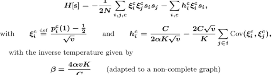
• (ii) automatic segmentation and BP fixed points identification
(a)
(b)
Fig. 5.1. Segmentation and BP fixed point identification (b) for Siouxfalls network (a).
In the first kind of experiments as in the preceding section, the fraction of observed variables ρ is varied and variables with time stamp in t0 (present) or t > t0 (future) are inferred, i.e. reconstructed or predicted respectively. In the type (ii) experiments, on one hand an automatic clustering of the data on reduced dimensional space is performed with machine learning techniques
developed in.7 On the other hand the BP fixed points obtained at ρ = 0 are
reduced dimensional space. A first set of data has been generated with the
traffic simulator “METROPOLIS”,2for a benchmark network called Siouxfalls
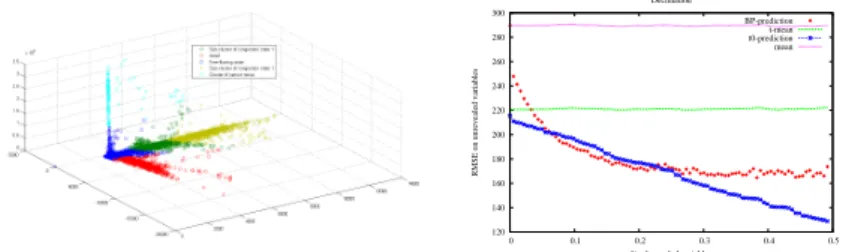
shown on Figure 5.1.a. An example of the automatic clustering of spatial con-figurations with the corresponding BP fixed points associated to free flow and congestion is shown on Figure 5.1.b. To perform tests on real data we have also considered a dataset consisting of travel time measured every 3 minutes over 2 years of a Highway segmented into 62 segments. For this case, we refined the mapping between travel time and latent traffic variables by using for a given travel time tt the index being defined by:
ui = f(tt)
def
= P (tti < tt),
using for each segment i = 1 . . . 62 a weighted cumulative travel time distribu-tion based on the automatic segmentadistribu-tion. On Figure 5.2.a is shown the result of this segmentation while on Figure 5.2.b is shown the result of a prediction with BP where error are computed on travel time.
120 140 160 180 200 220 240 260 280 300 0 0.1 0.2 0.3 0.4 0.5
RMSE on unrevealed variables
% of revealed variables Decimation BP-prediction t-mean t0-prediction mean
Fig. 5.2. (a) Automatic segmentation of Highway data. (b) BP prediction of 3 time
layers in future as a function of the fraction of observed variables at t0. Comparison
is made with a predictor combining recent available observations with historical time dependant mean.
6. Conclusion
In this paper we have reviewed some properties of the Belief-propagation al-gorithm and shown a promising approach for large scale applications in the context of traffic reconstruction and prediction. Concerning this application our method assume that traffic congestion is well represented by multiple dis-tant pattern superposition which needs validation with real data on networks. Our reconstruction schema seems to work already with simple underlying bi-nary indexes, but more work is needed for the dynamical part to be able to perform prediction.
References