HAL Id: hal-02916921
https://hal.archives-ouvertes.fr/hal-02916921
Submitted on 30 Nov 2020
HAL is a multi-disciplinary open access
archive for the deposit and dissemination of sci-entific research documents, whether they are pub-lished or not. The documents may come from
L’archive ouverte pluridisciplinaire HAL, est destinée au dépôt et à la diffusion de documents scientifiques de niveau recherche, publiés ou non, émanant des établissements d’enseignement et de
Some Rainbow Problems in Graphs Have Complexity
Equivalent to Satisfiability Problems
Olivier Hudry, Antoine Lobstein
To cite this version:
Olivier Hudry, Antoine Lobstein. Some Rainbow Problems in Graphs Have Complexity Equivalent to Satisfiability Problems. International Transactions in Operational Research, Wiley, In press. �hal-02916921�
Some Rainbow Problems in Graphs have
Complexity Equivalent to Satisfiability Problems
Olivier Hudry
LTCI, T´el´ecom Paris, Institut polytechnique de Paris 19, place Marguerite Perey, 91120 Palaiseau, France
& Antoine Lobstein
Centre National de la Recherche Scientifique Laboratoire de Recherche en Informatique, UMR 8623,
Universit´e Paris-Sud
Bˆatiment 650 Ada Lovelace, 91405 Orsay Cedex - France [email protected], [email protected]
June 29, 2020
Abstract
In a vertex-coloured graph, a set of vertices S is said to be a rainbow set if every colour in the graph appears exactly once in S. We inves-tigate the complexities of various problems dealing with domination in vertex-coloured graphs (existence of rainbow dominating sets, of rainbow locating-dominating sets, of rainbow identifying sets), includ-ing when we ask for a unique solution: we show equivalence between these complexities and those of the well-studied Boolean satisfiability problems.
Key Words: Graph theory, Complexity theory, Uniqueness of solution, Rainbow sets, Dominating codes, Locating-dominating codes, Identifying codes, Twin-free graphs
1
Introduction
We intend to locate in the classes of complexity several problems linked to the existence of rainbow dominating sets, of rainbow locating-dominating sets, and of rainbow identifying sets in a vertex-coloured graph, including when we ask for a unique solution. To this effect, we shall prove equivalence (up to polynomials) between the complexities of our problems and those of satisfiability problems.
This work is motivated by [1], [2], in particular their Theorem 2.1 (see Proposition 10 below) on the complexity of finding rainbow dominating sets in a vertex-coloured graph. Since locating-dominating sets and iden-tifying sets are particular classes of dominating sets, and since locating-domination and identification are popular nowadays (see the ongoing bibli-ography at [24]), it seems natural to try to extend this theorem to these two classes, including when considering domination at distance r and uniqueness of solution.
1.1 Vertex-Coloured Graphs
Let G = (V, E) be a finite, simple, undirected graph with vertex set V and edge set E, where an edge between v1 ∈ V and v2 ∈ V is indifferently
denoted by v1v2 or v2v1. The order of G is its number of vertices.
If Φ = {1, . . . , c} is a set of colours, then Gcol = (Vcol, E) denotes a
vertex-coloured graph (or simply coloured graph) obtained from G by giving one colour taken in Φ to every vertex v ∈ V , with each colour given to at least one vertex; here it is not necessary that two neighbour vertices receive different colours. When useful, we denote by φ(v) the colour given to v. A subset of vertices V∗ ⊆ V is said to be tropical if every colour appears at least once in V∗. It is said to be rainbow if every colour appears exactly
once in V∗; therefore, any rainbow set has c elements. When it is clear that
we are dealing with a coloured graph, we shall often drop the subscript col. Remark 1 Here, we stick to the definition of a rainbow subset which is used in [1] and [2], because our article is intended to prolong and widen the complexity result therein. However, a different terminology can be found in the literature: a rainbow subset can also designate a vertex subset where each colour appears at most once, whereas in a colourful subset, they appear exactly once; see, e.g., [3] or [9].
Since we shall study domination at distance r and, to this purpose, use the term rainbow r-domination, we have to mention that k-rainbow domi-nation is used with a different meaning in, e.g., [7].
1.2 More Definitions and Notation in Graphs
For any integer r ≥ 2, the r-th power of G is the graph Gr = (V, Er), with Er = {v
1v2: v1, v2∈ V, 0 < dG(v1, v2) ≤ r}.
For any integer r ≥ 1, and for every vertex v ∈ V , we denote by BG,r(v)
(and Br(v) when there is no ambiguity) the ball of radius r centered at v,
i.e., the set of vertices at distance at most r from v: Br(v) = {w ∈ V : 0 ≤ dG(v, w) ≤ r}.
Whenever v ∈ Br(w) (which is equivalent to w ∈ Br(v)), we say that v
and w r-dominate each other. When three vertices v, w, z are such that z ∈ Br(v) and z /∈ Br(w), we say that z r-separates v and w in G (note that
z = v is possible). A set of vertices is said to r-separate v and w if at least one of its elements does.
A subset of vertices V∗ will be indifferently called a set or a code, and
its elements codewords. We denote by IG,V∗,r(v) (and Ir(v) when there is no
ambiguity) the set of codewords that r-dominate v: IG,V∗
,r(v) = BG,r(v) ∩
V∗.
A code V∗ is said to be an r-dominating set or an r-dominating code
(r-D code for short) if for all v ∈ V , we have Ir(v) 6= ∅. One can also find
the terminology dominating set at distance r, or distance r dominating set. A code V∗ is said to be r-locating-dominating (r-LD for short) if for
all v ∈ V , we have Ir(v) 6= ∅, and for any two distinct non-codewords
v1, v2 ∈ V \ V∗, we have Ir(v1) 6= Ir(v2).
A code V∗ is said to be r-identifying (r-ID for short) if for all v ∈ V ,
we have Ir(v) 6= ∅, and for any two distinct vertices v1, v2 ∈ V , we have
Ir(v1) 6= Ir(v2).
In other words: every vertex must be r-dominated by at least one codeword for the three definitions; in addition, every pair of distinct non-codewords (respectively, vertices) must be r-separated by an r-LD (respec-tively, r-ID) code.
Two vertices v1, v2 ∈ V , v1 6= v2, are said to be r-twins if Br(v1) =
Br(v2). Dominating and locating-dominating codes exist for all graphs; on
the other hand, it is easy to see that a graph G admits an r-identifying code if and only if
∀v1 ∈ V, ∀v2∈ V, v16= v2: Br(v1) 6= Br(v2). (1)
A graph satisfying (1) is called r-identifiable or r-twin-free. The following useful remarks are quite trivial and need no proofs.
Remark 2 Let r ≥ 2 be any integer and G = (V, E) be a graph.
(a) A code V∗ is 1-dominating in Gr, the r-th power of G, if and only if it
is r-dominating in G.
(b) A code V∗ is 1-locating-dominating in Gr if and only if it is
r-locating-dominating in G.
Remark 3 A code V∗ is r-ID (respectively, r-LD) if and only if (a) for every vertex v ∈ V , Ir(v) 6= ∅, and (b) for every pair of distinct vertices
v1, v2 ∈ V (respectively, v1, v2∈ V \ V∗), we have
[Br(v1)∆Br(v2)] ∩ V∗ 6= ∅, (2)
where ∆ stands for the symmetric difference.
For the vast topic of 1-domination in graphs, see [18]. For locating-dominating and identifying codes, see the large bibliography at [24].
1.3 Satisfiability Problems
We consider a set X of n Boolean variables xi and a set C of m clauses; each
clause contains literals, a literal being a variable xi or its complement (or
negated variable) xi. A truth assignment for X sets the variable xito TRUE,
also denoted by T, and its complement to FALSE (or F), or vice-versa. A truth assignment is said to satisfy a clause if this clause contains at least one true literal, and to satisfy the set of clauses C if every clause contains at least one true literal. The following decision problems, for which the size of the instance is polynomially linked to n + m, are classical problems in complexity.
Problem SAT (Satisfiability):
Instance: A set X of variables, a collection C of clauses over X , each clause containing at least two different literals.
Question: Is there a truth assignment for X that satisfies C? Problem 3-SAT (3-Satisfiability):
Instance: A set X of variables, a collection C of clauses over X , each clause containing exactly three different literals.
Question: Is there a truth assignment for X that satisfies C?
1.4 A Short Background on Complexity
See, e.g., [4], [16], [23] or [26] for more on this topic; we assume that the reader is already familiar with the classes P, NP and co-NP, with NP-complete problems, and with the notion of polynomial transformation be-tween problems.
For problems which are not necessarily decision problems, a Turing re-duction from a problem π1 to a problem π2 is an algorithm A that solves π1
using a (hypothetical) subprogram S solving π2 such that, if S were a
poly-nomial algorithm for π2, then A would be a polynomial algorithm for π1.
Thus, in this sense, π2 is “at least as hard” as π1. A problem π is
NP-hard (respectively, co-NP-NP-hard) if there is a Turing reduction from some NP-complete (respectively, co-NP-complete) problem to π [16, p. 113].
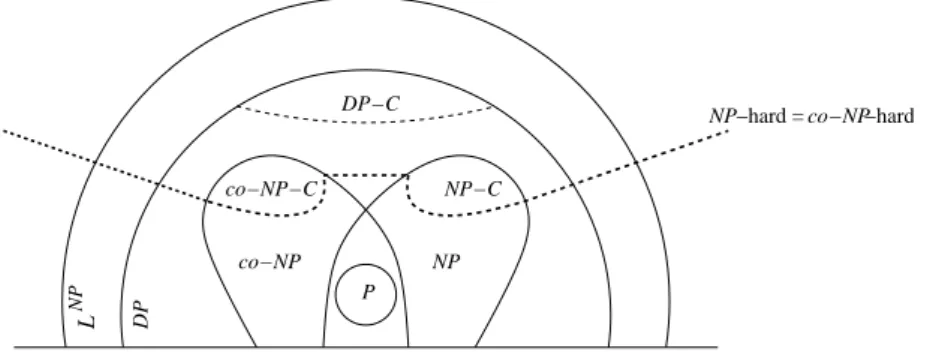
L NP co−NP NP NP−C P DP−C
NP−hard = co−NP−hard
co−NP−C
DP
Figure 1: Some classes of complexity.
Remark 4 Note that these two definitions, NP-hard and NP-hard, co-incide [16, p. 114].
The notions of completeness and hardness can be extended to classes other than NP or co-NP.
We shall also use the class LN P [23] (also denoted by PN P[O(log n)]or Θ 2),
which contains the decision problems which can be solved by applying, with a number of calls which is logarithmic with respect to the size of the instance, a subprogram able to solve an appropriate problem in NP (usually, an NP-complete problem); and the class DP [27] (or DIFP [5] or BH
2 [23], [28])
as the class of languages (or problems) L such that there are two languages L1 ∈ NP and L2 ∈ co-NP satisfying L = L1∩ L2. This class is not to be
confused with NP ∩ co-NP (see the warning in, e.g., [26, p. 412]); actually, DP contains NP ∪ co-NP and is contained in LN P. See Figure 1.
Membership to P, NP, co-NP, DP or LN P gives an upper bound on the
complexity of a problem (this problem is not more difficult than . . .), whereas a hardness result gives a lower bound (this problem is at least as difficult as . . .). Still, such results are conditional in some sense; if for example P = NP, they would lose their interest. But we do not know whether or where the classes of complexity collapse.
The decision problems SAT and 3-SAT are two of the basic and most well-known NP-complete problems [14], [16, p. 39, p. 46 and p. 259]. If we consider their variants U-SAT and U-3-SAT, where the question now is “Is there a unique assignment . . .”, the following result was proved in [22]. Proposition 5 [22, Th. 10] The decision problems U-SAT and U-3-SAT have equivalent complexities, up to polynomials.
Using results from [5] and [26, p. 415], it is then rather simple to obtain the following result.
Corollary 6 (a) The decision problems U-SAT and U-3-SAT are NP-hard. (b) The decision problems U-SAT and U-3-SAT belong to the class DP.
Remark 7 It is not known whether these problems are DP-complete. In [26, p. 415], it is said that “U-SAT is not believed to be DP-complete”. It is shown in [5] that there exists one oracle under which U-SAT is not DP-complete; and one oracle under which it is, if NP6=co-NP.
Note that uniqueness of solutions, which may be seen as part of the wider and rather unexplored issue of the number of solutions of a problem, had been studied earlier in a few papers (see, e.g., [5], [6], [8], [15], [17], [25]).
Let us now turn to the decision problems arising from the definitions given in Section 1.2; they are all stated for a fixed integer r ≥ 1:
Problem DCr / LDCr / IDCr ({r-Dominating / r-Locating-Dominating /
r-IDentifying} Code with bounded size): Instance: A graph G and an integer k.
Question: Does G admit an {dominating / locating-dominating / r-identifying} code of size at most k?
Proposition 8 Let r ≥ 1 be any integer.
(a) [16, p. 75 and p. 190, for r = 1], [19, Prop. 9] The decision problem DCr is NP-complete.
(b) [13, for r = 1], [10] The decision problem LDCr is NP-complete.
(c) [12, for r = 1], [10] The decision problem IDCr is NP-complete.
We have also results on the complexities of these problems when the question is about the uniqueness of the existence of a suitable set:
Proposition 9 Let r ≥ 1 be any integer.
(a) [21, Th. 25] The decision problems U-SAT and U-DCr have
equiva-lent complexities, up to polynomials.
(b) [20, Th. 20] The decision problems U-SAT and U-LDCr have
equiv-alent complexities, up to polynomials.
(c) [20, Th. 35] The decision problems U-SAT and U-IDCr have
equiv-alent complexities, up to polynomials.
As a consequence, by Corollary 6, the problems U-DCr, U-LDCr and
U-IDCr are NP-hard and belong to DP.
What about the same problems (with or without uniqueness of solution) when we consider coloured graphs? Note that it would not be interesting to ask whether there is, e.g., a tropical r-dominating code of size at most k in a coloured graph Gcol: in this case, we can simply observe that with a
graph coloured with only one colour, we are brought back to the basic prob-lem DCr. Much more interesting is to consider the existence of rainbow sets,
that is, to try to locate the following problems in the classes of complexity, and this is what we shall do in the sequel, with the additional requirement that all graphs be connected (see Remark 23):
Problem [U-]{RDCr/ RLDCr/ RIDCr} ([Unique] Rainbow {r-Dominating
/ r-Locating-Dominating / r-IDentifying} Code): Instance: A connected, coloured graph Gcol.
Question: Does Gcol admit a [unique] rainbow {r-dominating /
r-locating-dominating / r-identifying} code?
1.5 Outline of the Paper
In Sections 2.1–2.3, we give results on the NP-completeness of the problems RDC1, RLDC1 and RIDC1.
In Sections 2.4–2.6, we prove that the three problems U-RDC1,
U-RLDC1 and U-RIDC1 have a complexity which is equivalent to that of
U-SAT or U-3-SAT.
In some cases, we have results which hold even for paths or trees, or for graphs with a small number of occurrences for the colours appearing in the graph (typically, 2 or 3).
Then, in Sections 2.7–2.9, we shall extend our results to any r.
For the three types of codes, the general approach is the same, but the results slightly vary, and each type requires proofs which are different in their technical details, and cannot be merged. The starting point is the following result.
Proposition 10 [1, Th. 2.1], [2, Th. 2.1] The problem RDC1 is
NP-complete, even when restricted to coloured paths.
We give the proof, because it will be used and transformed for subsequent proofs. When, during the construction of a coloured graph, we say that a vertex has or is given a unique colour, we mean that this colour, at the end of the construction, appears exactly once. By extension, a vertex with unique colour is said to be unique, so that any unique vertex necessarily belongs to any rainbow set.
Proof of Proposition 10. In view of the subsequent proofs, we change slightly the proof from [1], [2]. The problem is clearly inside NP. We give a polynomial transformation from 3-SAT to RDC1. Let the set C of m
clauses over n variables x1, x2, . . ., xn be an instance of 3-SAT, for which
we may assume that each variable xi appears with its two forms, xi and xi
(otherwise, if it appears only in, say, its negated form, it suffices to take xi = F, and this variable and the clauses where it appears do not need to be
considered anymore).
We write C = {{ℓ1, ℓ2, ℓ3}, {ℓ4, ℓ5, ℓ6}, . . . , {ℓ3m−2, ℓ3m−1, ℓ3m}}, where
each literal ℓj is a variable xi or its complement xi. From this instance,
we define a coloured path P such that P admits a rainbow 1-dominating set if and only if there is an assignment of the variables that satisfies C. Example 12 below is intended to help to understand the notation.
middle M negative N b [1] c u1,4 1 1[0] 1,4 link L positive P artificial A
Figure 2: The gadget W1,4 (i = 1, i(1) = 4). The artificial vertex is
repre-sented by a black circle because it belongs to any rainbow set, the middle vertex by a square because it does not belong to any rainbow 1-dominating set, the other three vertices are unspecified.
We first construct a path
P0 = z1z2S1v1v2v3S2v4v5v6S3. . . Smv3m−2v3m−1v3mSm+1,
and we colour it in the following way. Vertices z1 and z2 are Blue (colour b).
Each vertex Ss, 1 ≤ s ≤ m + 1, receives a unique colour. Each vertex vi,
1 ≤ i ≤ 3m, which corresponds to the literal ℓiand is called a clausal vertex,
is coloured with the colour φ(vi) = i[0].
Next, we define a number of gadgets as follows. Whenever a pair of literals ℓp, ℓq satisfies ℓp = ℓq, we say that they are antithetic to each
other, and the same applies for the corresponding clausal vertices vp and vq.
For each literal ℓi, 1 ≤ i ≤ 3m, we consider the list of all the literals
ℓi(1), ℓi(2), . . . , ℓi(ki), that are antithetic to ℓi (by assumption, there is at
least one). To each literal ℓi(f ), 1 ≤ f ≤ ki, is associated a constraint gadget
Wi,i(f ) consisting of a path on five vertices, Ai,i(f ), Pi,i(f ), Mi,i(f ), Ni,i(f )
and Li,i(f ); vertex Ai,i(f ) is called artificial and has a unique colour, ui,i(f ); vertex Pi,i(f )is the positive vertex of Wi,i(f )and has colour i[f ]; vertex Mi,i(f ) is the middle vertex of Wi,i(f ), and φ(Mi,i(f )) = b ; vertex Ni,i(f ) is the
neg-ative vertex of Wi,i(f ) and has colour i[f −1]; vertex Li,i(f ) is the link vertex of Wi,i(f ) and has colour ci,i(f ) if i < i(f ), colour ci(f ),i otherwise.
Remark 11 (a) In P, the vertex z1 will not be linked to any vertex other
than z2; therefore, z1 or z2 necessarily belongs to any 1-dominating set
in P, and no Blue vertex other than z1 or z2 can belong to any rainbow
1-dominating set in P, i.e., no middle vertex.
(b) Every vertex Ss, 1 ≤ s ≤ m + 1, and every artificial vertex Ai,i(f ),
1 ≤ i ≤ 3m, 1 ≤ f ≤ ki, necessarily belong to any rainbow set.
(c) Every positive vertex Pi,i(ki) (which has colour i[ki]) is unique (see
Remark 13 below) and belongs to any rainbow set.
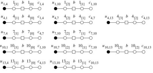
Example 12 Assume that ℓ1 = ℓ7 = ℓ13 = x1, ℓ4 = ℓ10 = x1 and there is
no other occurrence of x1 nor x1 in C. Figure 2 represents the gadget W1,4.
We have k1 = k7 = k13 = 2, k4 = k10 = 3, and ℓ1(1) = ℓ4, ℓ1(2) = ℓ10,
u4,1 4[0] 1 u1,4 [1] 1 10 [1] 10,1 13[1] 13 13,4 7 u7,4 [1] 7[0] c1,4 c1,4 4,7 c1,10 c4,13 c 10 b u u [0] 7 u7,10 [2] 7[1] 4 u4,7 4[1] 1 u1,10 1 c4,7 c1,10 10[2] 10 10,7 13 b u13,10 [2] c7,10 c10,13 c7,10 b 13 u 4 u4,13 4 u10,13 [3] 10[2] c10,13 c4,13 10 b [2] [1] [1] [2] [3] [0] [1] 4 [2] b b b b b b b b [0] [1]
Figure 3: The 12 gadgets from Example 12.
Figure 3 represents the 12 gadgets W1,4, W1,10, W4,1, W4,7, W4,13, W7,4,
W7,10, W10,1, W10,7, W10,13, W13,4, W13,10, produced by ℓ1 = x1, ℓ4 = x1,
ℓ7= x1, ℓ10= x1, ℓ13= x1.
Remark 13 One can see that the colours ci,i(f ) appear exactly twice, on the link vertices of the gadgets Wi,i(f ) and Wi(f ),i, and the same is true for the
colours i[0] (on one clausal vertex and in one gadget), i[1] (in two gadgets),
. . ., except for the “last” colour i[ki], which appears only once, on the positive
vertex Pi,i(ki) (in Figure 3, these colours are 1[2], 4[3], 7[2], 10[3] and 13[2]).
Only the Blue colour appears more than twice.
Finally, the path P is obtained by concatenating P0 and all the different
gadgets, and creating a unique vertex J, which is linked to the last vertex of the last gadget. The gadgets are ordered lexicographically; thus, in our example, we obtain P = P0W1,4W1,10W4,1. . . W13,10J.
Clearly, the construction is polynomial in the size of the instance of 3-SAT.
(a) We assume that there is a solution to 3-SAT, i.e., an assignment of the variables that satisfies C. We construct a rainbow 1-dominating set V∗ by putting the following vertices in V∗: (i) the vertex z
1 and all the unique
vertices; (ii) for every true literal ℓi, the clausal vertices vi (with colour i[0])
and, for every f ∈ {1, . . . , ki}, the positive vertices Pi,i(f ) ∈ Wi,i(f ) and
the link vertices Li,i(f ) ∈ Wi,i(f ); (iii) for every false literal ℓi and for every
f ∈ {1, . . . , ki}, the negative vertices Ni,i(f ) ∈ Wi,i(f ).
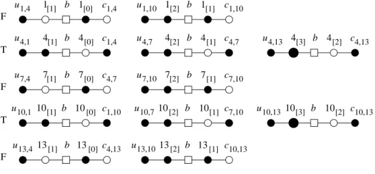
See Figure 4 for the gadgets of Example 12 with x1= FALSE. Note that
some vertices may be codewords for two reasons, (i) and (ii). In Figure 4, this is the case for the two positive vertices with colours 4[3] and 10[3] (the two large black vertices).
4 b u4,1 4[0] 1 b u1,4 [1] 1 10 [1] 10,1 13 b [0] 13,4 7 b u7,4 7[0] c1,4 c1,4 4,7 c1,10 c4,13 c 10 b u u 7 b u7,10 7[1] 4 b u4,7 4[1] 1 b u1,10 1 c4,7 c1,10 10[2] 10[1] 10,7 13 b u13,10 c7,10 c10,13 c7,10 b 13 u 4 b u4,13 4[2] u10,13 10[2] c10,13 c4,13 10 b F T F T F [2] [1] [1] [2] [3] [2] [0] [3] [1] [0] [1] [1] 13 [2]
Figure 4: In black, the codewords in the 12 gadgets from Example 12, with x1 = F, i.e., ℓ1= F, ℓ4 = T, ℓ7 = F, ℓ10= T, ℓ13= F.
We claim that V∗ is both rainbow and 1-dominating.
It is straightforward to check that the Blue colour, the unique colours and every colour i[f ], 1 ≤ i ≤ 3m, 0 ≤ f ≤ ki, appear exactly once in V∗.
All that remains to be checked are the colours ci,i(f ) of the link vertices in
the gadgets Wi,i(f ) and Wi(f ),i; since these two gadgets correspond to two literals that are antithetic, exactly one of them has been set TRUE by the assignment and exactly one of these two link vertices has been taken in the code. So V∗ is rainbow.
For every s ∈ {1, . . . , m}, the clausal vertices v3s−2 and v3s are
1-dominated by Ss ∈ V∗ and Ss+1 ∈ V∗, respectively; since by assumption
there is at least one true literal in each clause, the clausal vertex v3s−1 is
1-dominated by at least one clausal vertex which is a codeword. Inside a gadget, either the negative vertex, or the positive and link vertices, are code-words, and in both cases, every vertex is 1-dominated by V∗. Hence V∗ is
a 1-dominating set.
(b) We assume that there is a solution to RDC1, i.e., a rainbow
1-dominating set V∗. By Remark 11(a), no middle vertex can belong to V∗.
For every clausal vertex vi(with colour i[0]) that is a codeword, we assign
the value to the corresponding variable in such a way that ℓi is TRUE. We
claim that this (partial) assignment is consistent. Assume on the contrary that there is a pair of antithetic literals ℓpand ℓqreceiving the same value by
the assignment just defined, i.e., that the two antithetic clausal vertices vp
and vq are codewords. Assume without loss of generality that p < q. There
is an f ≥ 1 such that ℓq = ℓp(f ), and two gadgets, Wp,p(f ) and Wp(f ),p, both
containing a link vertex with the common colour cp,p(f ).
V∗. Assume first that f > 1. Because Mp,p(f ) ∈ V/ ∗, we have Np,p(f ) ∈
V∗, then P
p,p(f −1) ∈ V/ ∗ (because it has the same colour as Np,p(f )), then
Np,p(f −1) ∈ V∗ (to have one codeword that 1-dominates M
p,p(f −1)), . . .,
Np,p(1) ∈ V∗; but Np,p(1)has colour p[0], like vpwhich is also a codeword, and
this contradicts the fact that V∗ is rainbow. If f = 1, we get immediately
the same conclusion. So Lp,p(f ) must belong to V∗. But the same argument
can be applied to Wp(f ),pand Lp(f ),p, so the two link vertices, which have the same colour, are codewords, which is impossible. Therefore, the assignment defined by V∗ is valid. If necessary, we complete the assignment by giving
the value TRUE to the remaining unassigned variables.
Finally, this assignment satisfies 3-SAT because, for domination reasons, in each clause at least one clausal vertex belongs to V∗, i.e., at least one
literal is true.
So the answer to the initial instance of 3-SAT is YES if and only if the
answer to the constructed instance of RDC1 is YES. △
2
New Results
The first three Subsections of this Section are devoted to the problems RDC1, RLDC1 and RIDC1: we study one variant for RDC1, then we prove
that RLDC1 and RIDC1 are NP-complete, i.e., their complexity is
equiva-lent, up to polynomials, to that of, e.g., SAT.
The following three Subsections show that the same three problems with unique solution have complexity equivalent, up to polynomials, to that of U-SAT.
Then, in Subsections 2.7–2.9, we shall extend our results to RDCr,
RLDCr and RIDCr, for any r > 1.
2.1 Rainbow 1-Dominating Codes
We can go further and ask for a fixed number of occurrences for the colours appearing in the graph. With this number restricted to 2, we have a result of NP-completeness for coloured trees.
Proposition 14 The problem RDC1 is NP-complete, even when restricted
to trees where each colour appears at most twice.
Proof. We consider the construction in the proof of Proposition 10, where every middle vertex Mi,i(f ) in the gadget Wi,i(f ) had been given the colour b. As noticed in Remark 13, the Blue colour is the only colour appearing more than twice in the graph. To get rid of these multiple occurrences, we proceed as follows: (i) we delete the vertices z1, z2 and the edges z1z2 and z2S1;
(ii) for every middle vertex, we set φ(Mi,i(f )) = bi,i(f ) and we create the
1 S (a) r bi,i(f) r 1 S (b)
i,i(f) bi,i(f) i,i(f) 2,i,i(f) z’3,i,i(f) r r 1,i,i(f) z’ z’ 1,i,i(f) z 2,i,i(f) z i,i(f) z3,i,i(f) i,i(f)
Figure 5: (a) The graph Hi,i(f ) of Propositions 14 and 17, with its link to S1; (b) The graph Hi,i(f )′ of Propositions 19 and 28, with its link to S1.
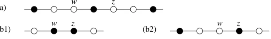
In black, the codewords, in white the non-codewords; black circles are forced codewords. z w w z (a) z (b2) (b1) w
Figure 6: In black, codewords, and in white, non-codewords. The vertices w and z are not 1-separated by any codeword.
Vi,i(f ) = {z1,i,i(f ), z2,i,i(f ), z3,i,i(f )}, Ei,i(f ) = {z1,i,i(f )z3,i,i(f ), z2,i,i(f )z3,i,i(f )},
together with the edge z3,i,i(f )S1. We set φ(z3,i,i(f )) = bi,i(f ) and give a new
colour, say ri,i(f )(for Red), to both z1,i,i(f )and z2,i,i(f ): see Figure 5(a). Now
the new graph is a tree and has no colour appearing more than twice. Since the Red vertices z1,i,i(f ) and z2,i,i(f ) must be 1-dominated by some codeword and cannot both belong to a rainbow set, we see that z3,i,i(f ) necessarily
belongs to any rainbow 1-dominating code (together with exactly one of z1,i,i(f ) and z2,i,i(f )); the consequence is that again, no middle vertex can belong to any rainbow 1-dominating set. The proof then goes exactly as for
Proposition 10. △
2.2 Rainbow 1-Locating-Dominating Codes
We now turn to 1-locating-dominating codes. We obtain the same results as for 1-dominating codes, one for paths without limitation on the occurrences of colours, one for trees where every colour appears at most twice.
Remark 15 On a path, the only configuration for a set which is 1-dominating and not 1-LD is given by Figure 6(a). One can see that this will never occur in the gadgets described in the proof of Proposition 10.
Proposition 16 The problem RLDC1 is NP-complete, even when restricted
Proof. We consider again the construction in the proof of Proposition 10. We duplicate the vertices Ss, 1 ≤ s ≤ m, so the path P0 now reads
P0 = z1z2S1S1′v1v2v3S2S2′v4v5v6S3S3′ . . . SmSm′ v3m−2v3m−1v3mSm+1,
where each S′
s is unique. The proof now goes exactly as previously:
(a) We construct a code V∗ by following the same rules (i)–(iii) as in
the Case (a) of the proof of Proposition 10. It is straightforward to see that all non-codewords are 1-dominated and 1-separated by the code in the gadgets (cf. Remark 15) as well as in P0, since the duplications avoid the
configurations of the type:
v3s−2 ∈ V∗, v3s−1 ∈ V/ ∗, v3s ∈ V/ ∗, Ss+1 ∈ V∗, v3s+1 ∈ V/ ∗, v3s+2 ∈ V/ ∗,
v3s+3∈ V∗
(cf. Figure 6(a)), that could exist in the previous construction. So V∗ is a
rainbow 1-LD set.
(b) Assume that there exists a rainbow 1-LD set V∗. Then we can apply
mutatis mutandis the Case (b) of the proof of Proposition 10, and construct
a valid assignment satisfying 3-SAT. △
Proposition 17 The problem RLDC1 is NP-complete, even when restricted
to trees where each colour appears at most twice.
Proof. Compared to the proof of Proposition 10, we duplicate the vertices Ss, 1 ≤ s ≤ m, like we did for Proposition 16, and, like for Proposition 14,
(i) we delete the vertices z1, z2 and the edges z1z2 and z2S1; (ii) for every
middle vertex, we set φ(Mi,i(f )) = bi,i(f )and we create the same graph Hi,i(f ) and the edge z3,i,i(f )S1, cf. Figure 5(a). Again, the new graph is a tree and
has no colour appearing more than twice, and z3,i,i(f ) necessarily belongs to any rainbow 1-LD code. The proof then goes like the previous ones. △
2.3 Rainbow 1-Identifying Codes
We now consider 1-identifying codes. We do not obtain a result which would be valid for paths, as was the case for the problems RDC1 and RLDC1, but
we do have a result on trees with occurrences of colours at most 2.
Remark 18 On a path, the only three configurations for a set which is dominating and not ID are given by Figure 6(a)–(b1)–(b2).
Proposition 19 The problem RIDC1 is NP-complete, even when restricted
to trees where each colour appears at most twice.
Proof. We consider again the construction for the proof of Proposition 10. (i) We triplicate the vertices Ss, 1 ≤ s ≤ m + 1, so the path P0 now
reads
where Ss′ and S′′s are unique. We also triplicate all the artificial vertices,
and the gadget Wi,i(f )now reads Ai,i(f )A′i,i(f )Ai,i(f )′′ Pi,i(f )Mi,i(f )Ni,i(f )Li,i(f ),
where A′i,i(f )and A′′i,i(f )are unique. Moreover, we triplicate the final vertex J by creating the unique vertices J′ and J′′, together with the edges JJ′ and
J′J′′.
(ii) For each middle vertex Mi,i(f ) ∈ Wi,i(f ), we create the unique
ver-tex Yi,i(f ), which is linked to Mi,i(f ): this will avoid the configuration given by Figure 6(b2), which appears for instance in the first gadget of Figure 4. The graph thus constructed is already not a path anymore.
(iii) We get rid of the multiple Blue colours of the middle vertices by deleting the vertices z1, z2 and the edges z1z2 and z2S1, and creating, for
every middle vertex Mi,i(f ), the graph Hi,i(f )′ = (Vi,i(f )′ , Ei,i(f )′ ), with
Vi,i(f )′ = {z1,i,i(f )′ , z2,i,i(f )′ , z3,i,i(f )′ }, E′
i,i(f )= {z1,i,i(f )′ z2,i,i(f )′ , z2,i,i(f )′ z3,i,i(f )′ },
together with the edge z′
3,i,i(f )S1. The colours are: φ(Mi,i(f )) = φ(z2,i,i(f )′ ) =
bi,i(f ) and φ(z′1,i,i(f )) = φ(z′3,i,i(f )) = ri,i(f ), see Figure 5(b). The only
ver-tex 1-separating z′
1,i,i(f ) and z2,i,i(f )′ is z′3,i,i(f ), so z3,i,i(f )′ belongs to every
1-identifying code. Then z′
1,i,i(f )cannot be a codeword, and z2,i,i(f )′ is a
code-word: observe already that here, we have no choice for these three vertices, unlike in the case of the graphs Hi,i(f ) for rainbow 1-D and 1-LD codes. The graph G just constructed is a tree, and no colour appears more than twice.
(a) We construct a code V∗ in G by following the same rules (i)–(iii) as
in the Case (a) of the proof of Proposition 10. In particular, every artificial vertex and every Yi,i(f ) are codewords, because they are unique, and inside a gadget, either the negative vertex, or the positive and link vertices, are code-words. It is easy to see why the three forbidden configurations of Figure 6 cannot appear in P0. Also thanks to the triplications, inside each gadget,
the artificial, positive and link vertices are all 1-dominated and 1-separated from all vertices by the artificial vertices.
If we have taken Ni,i(f ) in the code, then IG,V∗,1(N
i,i(f )) = {Ni,i(f )} and
IG,V∗
,1(Mi,i(f )) = {Ni,i(f ), Yi,i(f )}.
If we have taken Pi,i(f ) and Li,i(f ) in the code, then IG,V∗,1(N
i,i(f )) =
{Li,i(f )} and IG,V∗,1(M
i,i(f )) = {Pi,i(f ), Yi,i(f )}.
In both cases, IG,V∗
,1(Yi,i(f )) = {Yi,i(f )}, and all vertices are 1-dominated
and 1-separated by V∗: we can conclude that V∗ is a rainbow 1-identifying
set.
(b) Assume that there exists a rainbow 1-ID set V∗. Then we can still
use the same argument as in the Cases (b) of the proofs of Propositions 10 and 16, in particular because every middle vertex Mi,i(f ) still needs to be 1-dominated by a codeword belonging to Wi,i(f )\ {Mi,i(f )}, in order to be
2.4 Unique Rainbow 1-Dominating Codes
We are going to prove that U-SAT and U-RDC1 have equivalent
complexi-ties, up to polynomials; to this effect, we give a polynomial transformation from U-RDC1 to U-SAT (Proposition 20) and a polynomial transformation
from U-3-SAT to U-RDC1 (Proposition 21). One originality of this work is
that we need to go both ways; in particular, we need the first transformation because U-SAT, or U-3-SAT, is not sufficiently well located inside DP. Proposition 20 There exists a polynomial transformation from U-RDC1
to U-SAT.
Proof. We start from an instance of U-RDC1, a coloured graph G = (V, E)
of order n, where V = {v1, v2, . . . , vn}; the set {c1, c2, . . . , cγ} is the set
of γ colours used on V , and the number of occurrences of the colour ci
is λi; we set Λi = Σij=1λj for 1 ≤ i ≤ γ. Without loss of generality, we
can assume that V1 = {v1, . . . , vΛ1} is the set of vertices with colour c1,
Vi = {vΛi−1+1, . . . , vΛi} the set of vertices with colour ci (2 ≤ i ≤ γ), so
that the sets Vi, 1 ≤ i ≤ γ, partition V and the vertices are ranked by
increasing index of colour. For each vertex vi, we denote by v1i, . . ., v s(i) i the
s(i) neighbours of vi.
For each vertex vi, we create the variable xi. The set of clauses for
U-SAT is constructed in the following way:
(a) for every i ∈ {1, . . . , n}, we create the clause {xi, x1i, . . ., x s(i) i };
(b1) for every i ∈ {1, . . . , γ}, we create the clause {xj : vj ∈ Vi};
(b2) for every i ∈ {1, . . . , γ} and for every pair of vertices {vp, vq} ⊆ Vi,
p < q, we create the clause {xp, xq}.
Note that the number of variables and clauses is polynomial with respect to n, the order of G.
Now assume that we have a unique rainbow 1-dominating set V∗ in G.
Define the assignment A1 on the variables xi by A1(xi) = T if and only if
vi ∈ V∗. It is quite easy to see that the clauses described above are all
satisfied: the clauses in (a) because V∗ is 1-dominating, the clauses in (b1) because every colour appears at least once in V∗, and the clauses in (b2)
because every colour appears at most once in V∗.
Is A1 unique? Assume on the contrary that another assignment, A2,
also satisfies the constructed instance of U-SAT, and define the vertex set V+ by the rule v
i ∈ V+ if and only if A2(xi) = T. Since A1 6= A2, we have
V+6= V∗.
Because at least one literal is set TRUE by A2 in each clause from (a),
every vertex vi is in V+ or has a neighbour in V+, so the set V+ is
1-dominating; the clauses in (b1), when satisfied by A2, show that every colour
appears at least once in V+and the clauses in (b2), that every colour appears at most once in V+. Therefore, V+ is a rainbow 1-dominating set, but this contradicts the uniqueness of V∗.
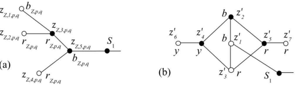
Figure 7: (a) The graph HZ,p,q for Proposition 21; (b) The graph HZ,p,q′
for Proposition 25, with lightened notation. Codewords are in black; all codewords are forced.
So a YES answer for U-RDC1 leads to a YES answer for U-SAT. Assume
now that the answer to U-RDC1 is negative. If it is negative because there
are at least two rainbow 1-D codes, then we have at least two assignments satisfying the instance of U-SAT: we have seen above how to construct a suitable assignment from a rainbow 1-D code, and different rainbow 1-D codes obviously lead to different assignments. If there is no rainbow 1-D code, then there is no assignment satisfying U-SAT, because such an assignment would give a rainbow 1-D code, as we have seen above from A2.
So in both cases, a NO answer to U-RDC1 implies a NO answer to U-SAT.
△ Proposition 21 There exists a polynomial transformation from U-3-SAT to U-RDC1. Moreover, in the connected graph constructed for this
transfor-mation, each colour appears at most thrice.
Proof. We consider again the construction for the proof of Proposition 10. (i) We delete the vertices z1, z2 and the edges z1z2 and z2S1.
(ii) For each pair of antithetic literals ℓp, ℓq, we add one vertex Zp,q
and the edges vpZp,q, Zp,qvq, and set φ(Zp,q) = bZ,p,q; since we assumed
that each variable xi appears under its two forms, xi and xi, every clausal
vertex is linked to at least one vertex of type Z. We then create the graph HZ,p,q with vertex set VZ,p,q = {zZ,1,p,q, zZ,2,p,q, zZ,3,p,q, zZ,4,p,q, zZ,5,p,q} and
edge set EZ,p,q= {zZ,1,p,qzZ,3,p,q, zZ,2,p,qzZ,3,p,q, zZ,3,p,qzZ,5,p,q, zZ,4,p,qzZ,5,p,q},
together with the edge zZ,5,p,qS1. We set φ(zZ,1,p,q) = φ(zZ,5,p,q) = bZ,p,qand
φ(zZ,2,p,q) = φ(zZ,3,p,q) = φ(zZ,4,p,q) = rZ,p,q. See Figure 7(a).
(iii) We give the colour bM,i,i(f ) to every middle vertex Mi,i(f ) ∈ Wi,i(f )
and we create the graph HM,i,i(f ) which is identical to the graph HZ,p,q,
except that we replace Z by M , p by i and q by i(f ), cf. Figure 7(a). The number of vertices linked to S1, apart from v1, is equal to the number
times the number of gadgets. One can already see that, in a rainbow 1-D code, in HZ,p,q and HM,i,i(f ), the vertices zZ,3,p,q and zZ,5,p,q on the one
hand, the vertices zM,3,i,i(f ) and zM,5,i,i(f ) on the other hand, are necessarily codewords, and the other vertices are not. As a consequence, no middle vertex and no vertex Zp,q can belong to any rainbow 1-D code.
In the constructed graph, each colour appears at most thrice.
As in Case (b) of the proof of Proposition 10 about the consistency of the assignment defined by a rainbow 1-D code, two antithetic causal vertices vpand vqcannot both be codewords, but, because Zp,qcannot belong to any
rainbow 1-D code, one of them is a codeword; this extends to all the vertices antithetic to vp, and so, all the clausal vertices corresponding to a variable x
belong to a rainbow 1-D code and none corresponding to x, or the other way round.
(a) Assume that there is a unique assignment satisfying the instance of 3-SAT. We build the set V∗ in the following way: (i) for every true literal ℓ
i,
the clausal vertex vi, with colour i[0], belongs to V∗; (ii) all the vertices
zZ,3,p,q, zZ,5,p,q, zM,3,i,i(f ) and zM,5,i,i(f ), and all the unique vertices belong
to V∗; (iii) for every true literal ℓ
i and f ∈ {1, . . . , ki}, the positive vertex
Pi,i(f ) ∈ Wi,i(f ) and the link vertex Li,i(f ) ∈ Wi,i(f ) belong to V∗; (iv) for
every false literal ℓi and f ∈ {1, . . . , ki}, the negative vertex Ni,i(f ) ∈ Wi,i(f )
belongs to V∗.
This is by now a routine task to check that V∗ is indeed a rainbow
1-dominating set. What is new is that, after the step (i) has been performed, i.e., once the decision has been made for all the clausal vertices, there is no choice left for the completion of a rainbow 1-D code. To prove this claim, all we have to check are the gadgets, since we have already seen that the step (ii) is forced. Consider the literal ℓ1, its first antithetic literal ℓ1(1), and
the gadget W1,1(1), and assume first that ℓ1= T. Then v1 ∈ V∗; this implies
that N1,1(1) ∈ V/ ∗, which implies in turn that L
1,1(1) ∈ V∗, P1,1(1) ∈ V∗ and
N1,1(2) ∈ V/ ∗. So we can go on in the same way for W
1,1(2): L1,1(2) ∈ V∗,
P1,1(2) ∈ V∗ and N
1,1(3) ∈ V/ ∗, and so on until we reach W1,1(k1), the last
gadget for ℓ1. Here, we have L1,1(k1) ∈ V
∗, P
1,1(k1) ∈ V
∗. We can repeat
this argument for all the literals set TRUE by the assignment. Assume now that ℓ1 = F. Then all the antithetic vertices of v1 are codewords, and
for 1 ≤ f ≤ k1, all the link vertices L1(f ),1 are codewords, none of the link
vertices L1,1(f )are codewords, all the negative vertices N1,1(f )are codewords,
none of the positive vertices P1,1(f −1)(when f = 1, this is v1) are codewords
—and the vertex P1,1(k1) is a codeword, because it is unique. This is true
for all false literals, and so we had no choice for the positive, negative and link vertices (and we know from the beginning that the artificial vertices are codewords and the middle vertices are not).
Now assume that there exists another rainbow 1-dominating set, V+. Then, denoting by VC the set of clausal vertices, we have: VC∩ V∗ 6= VC∩
V+. Setting the variable x to TRUE if and only if one clausal vertex v i
corresponding to one literal ℓi = x belongs to V+ (and we have seen that
then all the literals equal to x are in V+, and those equal to x are not), we obtain a second valid assignment, which as before satisfies the instance of 3-SAT. This is a contradiction.
(b) Assume that the answer to U-3-SAT is NO, either because there is no assignment satisfying the instance, or because there are at least two such assignments. In the latter case, this would lead however to two different rainbow 1-dominating sets. On the other hand, if no assignment exists, then no rainbow 1-D code V∗ exists, because V∗ would lead, as before, to a valid
assignment satisfying all the clauses —a contradiction.
Therefore, there is a YES answer to U-3-SAT if and only if there is a
YES answer to U-RDC1. △
Remark 22 We can be more specific than in the last sentence of the proof above: actually, the proof shows that there is zero, one, or more than one solution to the instance of 3-SAT if and only if there is zero, one, or more than one solution, respectively, in the constructed coloured graph; this proves that this construction could also have been used to provide a polynomial transformation from 3-SAT to RDC1, i.e., a proof of NP-completeness for
RDC1. This would not however give a result for paths, like Proposition 10,
nor for trees where each colour appears at most twice, like Proposition 14. Remark 23 If we allow unconnected graphs, then it is easy to build a graph where each colour appears at most twice, by using isolated vertices with a colour that we do not wish elsewhere: instead of building the graph HZ,p,q so
that the vertex Zp,q with the colour bZ,p,qcannot be a codeword, we can simply
create one isolated vertex with this colour. The same is true for HM,i,i(f ).
2.5 Unique Rainbow 1-Locating-Dominating Codes
We have the same results for unique rainbow 1-LD codes as for unique rainbow 1-D codes.
Proposition 24 There exists a polynomial transformation from U-RLDC1
to U-SAT.
Proof. The method is the same as in the proof of Proposition 20, and uses the characterization of LD codes in Remark 3, and in particular (2). Only the clauses in (a) will change, in order to fit the required location-domination property: compared to the previous construction, the clauses in (b1) and (b2) are unchanged, and, keeping the same notation, the new clauses read:
(a1) for every i ∈ {1, . . . , n}, we create the clause {xi, x1i, . . ., x s(i)
i }: here
again, we translate the fact that we look for 1-dominating sets;
(a2) for each pair of vertices vp and vq, we consider the set B1(vp)∆
the clause {xp, xq, xh1, xh2, . . . , xht}; we shall say that {xp, xq} is the first
part of the clause, and {xh1, xh2, . . . , xht} its second part, which exists only
when t > 0 and may contain variables also appearing in the first part, a fact which is unimportant.
Assume that we have a unique rainbow 1-LD code, V∗; as previously,
from V∗ we define an assignment A
1. Then the clauses in (a1) are satisfied
by A1, because V∗is 1-dominating. And the clauses in (a2) also are satisfied:
if at least one of vp and vqis in V∗, then the first part of the clause contains
a true literal; if neither vp nor vq is a codeword, then at least one vertex in
B1(vp)∆ B1(vq) must be, and the second part of the clause contains a true
literal.
The end of the proof is similar to the proof of Proposition 20. △ Proposition 25 There exists a polynomial transformation from U-3-SAT to U-RLDC1. Moreover, in the connected graph constructed for this
trans-formation, each colour appears at most thrice.
Proof. Compared to the transformation from U-3-SAT to U-RDC1
(Propo-sition 21), and after we have duplicated the vertices Ss, 1 ≤ s ≤ m, like we
did for going from Proposition 10 to Proposition 16, the differences are: (i) for each pair of antithetic literals ℓp, ℓq, we create three vertices Zp,q,
Z′
p,q and Zp,q′′ , and the edges vpZp,q, Zp,qZp,q′′ , Zp,q′′ Zp,q′ , and Zp,q′ vq; the
ver-tices Zp,q and Zp,q′ are given the colours bZ,p,q and bZ′,p,q, respectively, while
Zp,q′′ is unique; then, to deal with Zp,q, we create the graph HZ,p,q′ with
ver-tex set {z′
Z,i,p,q : 1 ≤ i ≤ 7} represented in Figure 7(b) where, for simplicity,
we indicate only the second subscript of the vertices z′
Z,i,p,q. The vertex
zZ,1,p,q′ is linked to S1 and the colours are: φ(zZ,1,p,q′ ) = φ(zZ,2,p,q′ ) = bZ,p,q,
φ(z′
Z,3,p,q) = φ(zZ,5,p,q′ ) = φ(z′Z,7,p,q) = rZ,p,q and φ(zZ,4,p,q′ ) = φ(z′Z,6,p,q) =
yZ,p,q(for Yellow). Again for simplicity, we drop the subscripts of the colours
in Figure 7(b). Similarly, we create the graph H′
Z′,p,q for Zp,q′ .
(ii) We give the colour bM,i,i(f ) to every middle vertex Mi,i(f ) ∈ Wi,i(f )
and we create the graph H′
M,i,i(f ) which is identical to the graph HZ,p,q′ ,
except that we replace Z by M , p by i and q by i(f ), cf. Figure 7(b). Remark 26 Assume that V∗ is a rainbow 1-LD code. Because z′
Z,2,p,q and
z′
Z,3,p,q have the same neighbours, at least one of them must belong to V∗;
if however z′
Z,3,p,q ∈ V∗, then zZ,7,p,q′ cannot be 1-dominated by V∗. So
z′
Z,2,p,q ∈ V∗, zZ,3,p,q′ ∈ V/ ∗, and zZ,1,p,q′ ∈ V/ ∗. It is then straightforward to
check that necessarily the Yellow and Red codewords are z′
Z,4,p,q and z′Z,5,p,q,
respectively (and z′
Z,6,p,q∈ V/ ∗, zZ,7,p,q′ ∈ V/ ∗).
As a consequence, no middle vertex and no vertex Zp,q, Zp,q′ can belong
to any rainbow 1-LD code.
In the constructed graph, each colour appears at most thrice.
As in Case (b) of the proof of Proposition 21 about the consistency of the assignment defined by a rainbow 1-D code, two antithetic causal vertices
vp and vq cannot both be codewords; on the other hand, because neither
Zp,q nor Zp,q′ can belong to any rainbow 1-LD code, one of vp and vq is a
codeword, so that Zp,qand Zp,q′ are 1-separated by a codeword. This extends
to all the vertices antithetic to vp; so, all the clausal vertices corresponding
to a variable x belong to a rainbow 1-LD code and none corresponding to x, or the other way round.
The proof then follows the lines of the proof of Proposition 21. △
2.6 Unique Rainbow 1-Identifying Codes
We obtain a better result for unique rainbow 1-ID codes, in the sense that, starting from U-3-SAT, we are able to construct a coloured graph where each colour appears at most twice. But first we go from U-RIDC1 to U-SAT:
Proposition 27 There exists a polynomial transformation from U-RIDC1
to U-SAT.
Proof. Same technique as for Propositions 20 and 24. We start from a twin-free graph and define the clauses of type (a) as follows (it relies on the characterization of Remark 3):
(a1) for every i ∈ {1, . . . , n}, we create the clause {xi, x1i, . . ., x s(i) i };
(a2) for each pair of vertices vp and vq, we consider the set B1(vp)∆
B1(vq) = {vh1, vh2, . . . , vht}; because G is twin-free, we have t > 0. Then we
construct the clause {xh1, xh2, . . . , xht}, which is simply the second part of
the clause defined in the Case (a2) of the proof of Proposition 24.
The end of the proof is similar to the previous two proofs of this type. △ Proposition 28 There exists a polynomial transformation from U-3-SAT to U-RIDC1. Moreover, in the connected graph constructed for this
trans-formation, each colour appears at most twice.
Proof. With respect to the original construction, we triplicate the vertices Ss, 1 ≤ s ≤ m + 1, all the artificial vertices, and the final vertex J. For
each pair of antithetic literals ℓp, ℓq, we add two vertices Zp,q, Zp,q′ and the
edges vpZp,q, Zp,qvq and Zp,qZp,q′ , and set φ(Zp,q) = bZ,p,q; the vertex Zp,q′ is
unique. We give the colour bM,i,i(f ) to every middle vertex Mi,i(f ) ∈ Wi,i(f ).
For each middle vertex Mi,i(f ), we create the unique vertex Yi,i(f ), which is linked to Mi,i(f ).
For every pair of antithetic literals ℓp, ℓq, we create the graph HZ,p,q′
given by Figure 5(b), with the edge z′
Z,1,p,qS1, and for every middle vertex
Mi,i(f ), the similar graph H′
M,i,i(f ) and the edge z′M,1,i,i(f )S1.
We have already observed that z′
Z,2,p,qand zZ,3,p,q′ , not zZ,1,p,q′ , necessarily
belong to any rainbow 1-ID code, and the same is true for z′
M,2,i,i(f ) and
z′
M,3,i,i(f ), and zM,1,i,i(f )′ . Then one can see that exactly one of the two
The end of the proof is the same as that of Propositions 21 and 25. △
2.7 Generalization to r >1: Dominating Sets
We start with an easy lemma, which is actually common to the three prob-lems.
Lemma 29 Let r ≥ 2 be any integer. There is a polynomial transformation from U-RDCr to U-SAT, from U-RLDCr to U-SAT, and from U-RIDCr to
U-SAT.
Proof. Let G = (V, E) be a coloured graph, assumed to be r-twin-free in the case of U-RIDCr, and consider Gr, the r-th power of G. By Remark 2, there
is a unique rainbow 1-D code (respectively, 1-LD code, 1-ID code) in Gr if
and only if there is a unique rainbow r-D code (respectively, r-LD code, r-ID code) in G. Therefore, we have a first transformation, from U-RDCr
to U-RDC1, from U-RLDCr to U-RLDC1, or from U-RIDCr to U-RIDC1.
Then we apply Propositions 20, 24 and 27, with their transformations from
U-RDC1 to U-SAT, from U-RLDC1 to U-SAT, from U-RIDC1 to U-SAT,
and the transitivity of polynomial transformations. △
Then we turn to rainbow r-dominating sets.
Proposition 30 Let r ≥ 2 be any integer. There is a polynomial transfor-mation from U-RDC1 to U-RDCr.
Proof. Let G = (V, E) be any instance of U-RDC1, that is, any coloured
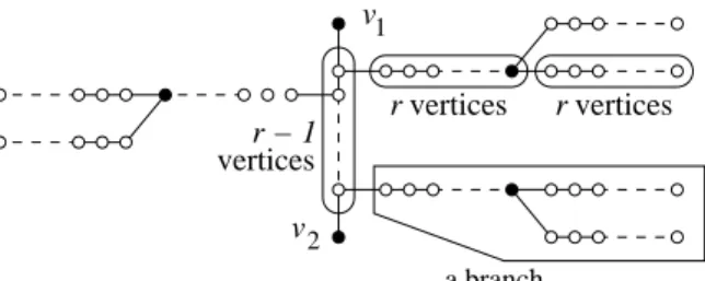
graph, and let e = v1v2 be any edge in G. Let
Ve§= {αe,i: 1 ≤ i ≤ r − 1} ∪ {βe,i,j : 1 ≤ i ≤ r − 1, 1 ≤ j ≤ 3r},
Ee§= {v1αe,1, αe,1αe,2, . . . , αe,r−2αe,r−1, αe,r−1v2} ∪
{αe,iβe,i,1, βe,i,1βe,i,2, . . . , βe,i,rβe,i,r+1, . . . , βe,i,2r−1βe,i,2r : 1 ≤ i ≤ r − 1}
∪ {βe,i,rβe,i,2r+1, βe,i,2r+1βe,i,2r+2, . . . , βe,i,3r−1βe,i,3r : 1 ≤ i ≤ r − 1},
see Figure 8. For i ∈ {1, . . . , r − 1}, the vertex αe,i and all the vertices βe,i,j,
1 ≤ j ≤ 3r, (i.e., the branch linked to αe,i) receive the colour bi,e, which will
appear nowhere else. Then we set
V§= V ∪ (∪e∈EVe§), E§= ∪e∈EEe§,
and G§ = (V§, E§) is the instance of U-RDC
r (the colours in V remain the
same). Note in particular that any two vertices at distance 1 in G are at distance r in G§; this is why we shall say that the edge e is dilated.
We claim that an instance of U-RDC1 is positive if and only if the
corre-sponding constructed instance of U-RDCr is.
(a) First, we assume that there is a YES answer for U-RDC1: there is a
unique rainbow 1-dominating code V∗
vertices r v vertices r r − 1 vertices v 1 2 a branch
Figure 8: How the edge e = v1v2 ∈ E gives Ve§ and Ee§. The black vertices
on the branches are the vertices βe,i,r.
the (r − 1)|E| vertices βe,i,r, e ∈ E, 1 ≤ i ≤ r − 1 (they are represented as
black vertices in Figure 8). Note that W r-dominates exactly V§\ V . Then
V1+= V∗
1 ∪ W is a rainbow r-dominating set in G§. Is V1+ unique?
Assume on the contrary that V2+ is another rainbow r-D code in G§.
Because βe,i,r is the only vertex r-dominating the two extremities of its
branch, βe,i,2r and βe,i,3r, and for rainbow reasons, we have
(V§\ V ) ∩ V2+= W. Let V∗
2 = V2+\ W = V2+ ∩ V . Clearly, V2∗ is a rainbow 1-D code in G,
different from V∗
1, a contradiction.
(b) Next, we assume that the answer to U-RDC1 is NO: either there is
no rainbow 1-dominating code in G, or there is more than one. In the latter case, we have more than one rainbow r-D code in G§: simply add the set W
to the codes in G. So we assume that we are in the first case. If there is a rainbow r-D code V+ in G§, then again V+\ W would be a rainbow 1-D
code in G, a contradiction. In all cases, the answer to U-RDCr is also NO.
△ Corollary 31 Let r ≥ 1 be any integer. The decision problem RDCr is
NP-complete.
Proof. We can use Remark 22 here: the above proof of Proposition 30 shows that there is zero, one, or more than one solution to the instance of U-RDC1
if and only if there is zero, one, or more than one solution, respectively, in the constructed coloured graph G§; this proves that we have a
polyno-mial transformation from RDC1 to RDCr, i.e., a proof of NP-completeness
for RDCr, since RDC1 is NP-complete (Propositions 10 or 14) and RDCr
obviously belongs to NP. △
However, a better result can be obtained.
Proposition 32 Let r ≥ 1 be any integer. The decision problem RDCr is
q 1,1 p 1 q h,r−1 p 2 p p 3 h
G
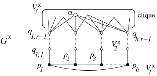
α clique x q1,r−1 3 x V 2 x V 1 x VFigure 9: The graph G×. Black vertices are forced codewords. White ver-tices are forced non-codewords.
Proof. Apply the construction from the proof of Proposition 30, which yields a tree, to the path constructed in the proof of Proposition 10. △ For r > 1, we do not have results with a fixed number of occurrences of the colours. We can now conclude for the problem U-RDCr.
Proposition 33 Let r ≥ 1 be any integer. The decision problems U-SAT and U-RDCr have equivalent complexities, up to polynomials.
Proof. There is a polynomial transformation from U-3-SAT to U-RDC1
(Proposition 21), from U-RDC1 to U-RDCr (Proposition 30), and from
U-RDCr to U-SAT (Lemma 29). △
2.8 Generalization to r >1: Locating-Dominating Sets
In order to dilate the edges, we need, as with the branches and the set W in the case of dominating codes, a graph which has all its codewords (and non-codewords) forced.
Let r ≥ 2 and h = 2r + 1. Let G×1 = (V1×, E1×) be the cycle of length h, with V1×= {pi : 1 ≤ i ≤ h}. Then we construct G×2 = (V2×, E2×), with V2×=
{qi,j : 1 ≤ i ≤ h, 1 ≤ j ≤ r − 1} and E2×= ∪1≤i≤h{qi,jqi,j+1 : 1 ≤ j ≤ r − 2}.
The set of edges between G×1 and G×2 is E1,2× = {piqi,1 : 1 ≤ i ≤ h}. Next,
we construct G×3 = (V3×, E3×) with V3× = {si : 1 ≤ i ≤ 2h− 1 − (r − 1)h}
and E3×= {si1si2 : 1 ≤ i1 < i2 ≤ |V3×|}, i.e., G×3 is a clique.
We set V×= V×
1 ∪ V2×∪ V3×, see Figure 9.
In order to define the set E2,3× of edges between {qi,r−1 : 1 ≤ i ≤ h}
and V3×, we introduce, for every vertex v ∈ V2×∪ V3×, the signature of v as the set Br(v) ∩ V1× of the elements of the cycle that r-dominate v, and we
wish to have nonempty and distinct signatures. Since (a) the h vertices in V1× can provide 2h− 1 such signatures;
(b) |V2×∪ V×
3 | = |V2×| + |V3×| = 2h− 1;
(c) because h is sufficiently large, the vertices qi,j in V2× have nonempty and
(d) a vertex in V3× which is linked (respectively, not linked) to qi,r−1 is at
distance equal to (respectively, greater than) r from pi;
we can see that it is possible to construct E2,3× in such a way that the vertices in V3×have nonempty signatures which are different inside V3×, and different from those for V2×. In particular, in V3×there is a vertex which has signature equal to V1×; we denote this vertex by α. Note also that we could not have more vertices with this signature property.
We set E× = E×
1 ∪ E1,2× ∪ E2× ∪ E2,3× ∪ E3× and G× = (V×, E×). The
order of G×is n×= 2h− 1 + h. Then we give colours to G×in the following
way: the vertices in V1×\ {pr+1} are unique, the other vertices share the
Blue colour.
Lemma 34 The only rainbow r-LD code in G× is the cycle V× 1 .
Proof. Every rainbow r-LD code must contain the h − 1 unique vertices, plus one Blue vertex. Consider the four vertices w1, w2, w3, w4 in V3× with
signatures {p1}, {p2}, {p1, pr+1} and {p2, pr+1}, respectively. No vertex
in V3×, no vertex in V2×, can r-separate w1 and w3, w2 and w4, only pr+1
can. On the other hand, V1× is a rainbow r-LD code, because now the signatures are simply the sets IG×,V×
1 ,r(v), for v ∈ V
×
2 ∪ V3×= V×\ V1×: by
construction, they are all nonempty and distinct. △
Proposition 35 Let r ≥ 2 be any integer. There is a polynomial transfor-mation from U-RLDC1 to U-RLDCr.
Proof. We start from an instance of U-RLDC1, i.e., a coloured graph
G = (V, E) of order n.
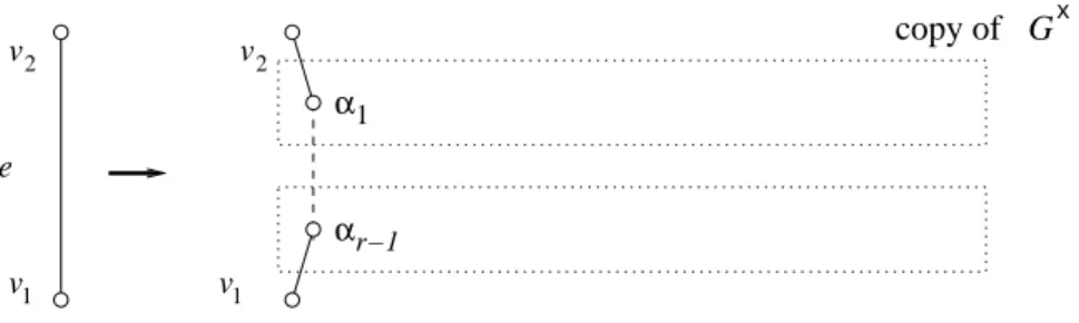
For each edge e = v1v2 ∈ E that we want to dilate, we “paste” r − 1
copies of the graph G×, by deleting the edge e = v
1v2 and creating the edges
v1α1, α1α2, . . ., αr−1v2, where the αi’s are copies of the vertex α in G×;
see Figure 10. We denote by G§ = (V§, E§) the graph thus constructed.
The colours in G§ are given as follows: the colours in V are unchanged, the
vertices in each copy of V1×\ {pr+1} are unique, and the other vertices in
each copy of G× share the colour b
i, i.e., one different colour for each copy.
The order of G§is |V |+|E|(r−1)(2h+h−1). Since r, hence h = 2r+1, is
fixed, this does not affect the polynomiality of our construction with respect to n, the order of G.
We claim that there is a unique rainbow 1-LD code in G if and only if there is a unique rainbow r-LD code in G§.
(a) Assume first that there is a unique rainbow 1-LD code V∗
1 in G. We
construct the following code V1+ in G§: we add to V∗
1 the set W of all the
vertices in all the cycles G×1 in all the copies of G×. Note that these vertices
in W do not r-dominate any vertex in V . Obviously, V1+ is a rainbow r-LD code in G§. Is it unique?
αr−1 α1 v1 v1 e G v2 v2 x copy of
Figure 10: How the edge e = v1v2∈ E is dilated for Proposition 35.
The argument is similar to the one for dominating codes: assume on the contrary that V2+ is another rainbow r-LD code in G§. The intersection of
V§\ V with V+
2 is equal to W , because, since the vertices in V do not
r-separate between any vertices in any copy of the clique G×3, except possibly the vertex α, we can still apply the argument of Lemma 34, and it is still true that, in addition to the unique vertices, we must take as codewords all the copies pi
r+1, 1 ≤ i ≤ |E|(r − 1), of the vertex pr+1. Let V2∗ = V2+\ W =
V2+∩ V . Clearly, V∗
2 is a rainbow 1-LD code in G, different from V1∗, a
contradiction.
(b) Next, we assume that the answer to U-RLDC1 is NO: either there is
no rainbow 1-LD code in G, or there is more than one. In the latter case, we have more than one rainbow r-LD code in G§: simply add the set W to
the codes in G. So we assume that we are in the first case. But if there is a rainbow r-LD code V+ in G§, then again V+\ W would be a rainbow 1-LD code in G, a contradiction. In both cases, the answer to U-RLDCr is
also NO. △
The following consequences are immediate.
Corollary 36 Let r ≥ 1 be any integer. The decision problem RLDCr is
NP-complete.
Proposition 37 Let r ≥ 1 be any integer. The decision problems U-SAT and U-RLDCr have equivalent complexities, up to polynomials.
2.9 Generalization to r >1: Identifying Sets
Lemma 38 Let r ≥ 1 be any integer. Let G = (V, E) be the (non coloured) path β1β2. . . β3r+1. Then V∗= {βr+1, . . . , β2r} is included in any r-identifying
code.
Proof. Apply Lemma 4 in [11] with n = 3r + 1. Note that β2r+1 also
belongs to any r-identifying code, but we do not need it for our purpose. △ We colour the previous path in the following way: for i ∈ {1, . . . , r}, φ(βi) =
Lemma 39 The coloured path defined above admits V+= {βi: r + 1 ≤ i ≤
3r + 1} as its unique rainbow r-identifying code.
Proof. A rainbow r-ID code must contain V∗ and the unique vertices. The
vertices βi, 1 ≤ i ≤ r, cannot be codewords for rainbow reasons. It is easy
to check that V+ is indeed a rainbow r-ID code, and is the only one. △ Proposition 40 Let r ≥ 2 be any integer. There is a polynomial transfor-mation from U-RIDC1 to U-RIDCr.
Proof. Let G = (V, E) be any instance of U-RIDC1, that is, any coloured
graph, and let e = v1v2 be any edge in G. Let
Ve§= {βe,i,j: 1 ≤ i ≤ r − 1, 1 ≤ j ≤ 3r + 1},
Ee§= {v1βe,1,1, βe,1,1βe,2,1, . . . , βe,r−2,1βe,r−1,1, βe,r−1,1v2} ∪
{βe,i,1βe,i,2, βe,i,2βe,i,3, . . . , βe,i,3rβe,i,3r+1: 1 ≤ i ≤ r − 1},
i.e., in order to dilate all the edges, we have split every edge e with r − 1 vertices βe,i,1 which are the starting points of copies of the path defined for
Lemma 38. Then we set
V§= V ∪ (∪e∈EVe§), E§= ∪e∈EEe§,
and G§ = (V§, E§). The set V keeps its colours unchanged. Each path is
coloured as was done for Lemma 39, with its specific colours that will be nowhere else. Note that the set {βe,i,j : r + 1 ≤ j ≤ 3r + 1} r-dominates
exactly the set {βe,i,j : 1 ≤ j ≤ 3r + 1}, for all e and i.
We claim that the instance of U-RIDC1 we started from, is positive if
and only if the coloured graph G§ admits a unique rainbow r-ID code.
(a) First, we assume that there is a unique rainbow 1-ID code V1∗ in G. Let W be the set consisting of the |E|(2r + 1)(r − 1) vertices βe,i,j, e ∈ E,
1 ≤ i ≤ r − 1, r + 1 ≤ j ≤ 3r + 1. Note that W r-dominates exactly V§\ V .
Then V1+= V1∗∪ W is a rainbow r-identifying set in G§. Is V+
1 unique?
Assume on the contrary that V2+ is another such code in G§. We have
(V§\ V ) ∩ V+
2 = W . Let V2∗= V2+\ W = V2+∩ V . Clearly, V2∗ is a rainbow
1-ID code in G, different from V1∗, a contradiction.
(b) Next, we assume that the answer to U-RIDC1 is NO: either there is
no rainbow 1-ID code in G, or there is more than one. In the latter case, we have more than one rainbow r-ID code in G§: simply add the set W to the codes in G. So we assume that we are in the first case. If there is a rainbow r-ID code V+in G§, then again V+\ W would be a rainbow 1-ID code in G,
a contradiction. In both cases, the answer to U-RIDCr is NO. △
As previously, we have the following easy consequences.
Corollary 41 Let r ≥ 1 be any integer. The decision problem RIDCr is
Proposition 42 Let r ≥ 1 be any integer. The decision problem RIDCr is
NP-complete, even when restricted to coloured trees.
Proposition 43 Let r ≥ 1 be any integer. The decision problems U-SAT and U-RIDCr have equivalent complexities, up to polynomials.
3
Conclusion
We recapitulate all the above results and summarize them in Table 1 below. (i) The decision problem RDC1 was known to be NP-complete, even
for paths [1], [2]. We proved that it is NP-complete, even when restricted to trees where each colour appears at most twice (Proposition 14). For all r ≥ 2, we proved that the decision problem RDCr is NP-complete, even for
trees (Proposition 32).
We proved that the decision problems U-RDC1 and U-SAT have
equiva-lent complexities, up to polynomials, and settled the case when each colour appears at most thrice (Propositions 20 and 21). For all r ≥ 2, we proved that the decision problems U-RDCr and U-SAT have equivalent
complex-ities, up to polynomials (Proposition 33). Using Corollary 6, we have the following result.
Proposition 44 For all r ≥ 1, the decision problem U-RDCr is NP-hard
and belongs to the class DP.
(ii) We proved that the decision problem RLDC1 is NP-complete, even
for paths (Proposition 16), and when restricted to trees where each colour appears at most twice (Proposition 17). For all r ≥ 2, we proved that the decision problem RLDCr is NP-complete (Corollary 36).
We proved that the decision problems U-RLDC1and U-SAT have
equiv-alent complexities, up to polynomials, and settled the case when each colour appears at most thrice (Propositions 24 and 25). For all r ≥ 2, we proved that the decision problems U-RLDCr and U-SAT have equivalent
complex-ities, up to polynomials (Proposition 37). Using Corollary 6, we have the following result.
Proposition 45 For all r ≥ 1, the decision problem U-RLDCr is NP-hard
and belongs to the class DP.
(iii) We proved that the decision problem RIDC1is NP-complete, even when
restricted to trees where each colour appears at most twice (Proposition 19). For all r ≥ 2, we proved that the decision problem RIDCr is NP-complete,
even for trees (Proposition 42).
We proved that the decision problems U-RIDC1 and U-SAT have
equiv-alent complexities, up to polynomials, and settled the case when each colour appears at most twice (Propositions 27 and 28). For all r ≥ 2, we proved