Statistical Characterization of Round-Trip Times with Nonparametric Hidden Markov Models

HAL Id: hal-02010099

https://hal.archives-ouvertes.fr/hal-02010099

Submitted on 6 Feb 2019

HAL is a multi-disciplinary open access

archive for the deposit and dissemination of

sci-entific research documents, whether they are

pub-lished or not. The documents may come from

teaching and research institutions in France or

abroad, or from public or private research centers.

L’archive ouverte pluridisciplinaire HAL, est

destinée au dépôt et à la diffusion de documents

scientifiques de niveau recherche, publiés ou non,

émanant des établissements d’enseignement et de

recherche français ou étrangers, des laboratoires

publics ou privés.

Statistical Characterization of Round-Trip Times with

Nonparametric Hidden Markov Models

Maxime Mouchet, Sandrine Vaton, Thierry Chonavel

To cite this version:

Maxime Mouchet, Sandrine Vaton, Thierry Chonavel. Statistical Characterization of Round-Trip

Times with Nonparametric Hidden Markov Models. IFIP/IEEE IM 2019 Workshop: 4th International

Workshop on Analytics for Network and Service Management (AnNet 2019), Apr 2019, Washington

DC, United States. �hal-02010099�

Statistical Characterization of Round-Trip Times

with Nonparametric Hidden Markov Models

Maxime Mouchet, Sandrine Vaton

IMT Atlantique, IRISA, UBL Brest, France

Thierry Chonavel

IMT Atlantique, Lab-STICC, UBL Brest, France

Abstract—The study of round-trip time (RTT) measurements on the Internet is of particular importance for improving real-time applications, enforcing QoS with traffic engineering, or de-tecting unexpected network conditions. On large timescales, from 1 hour to several days, RTT measurements exhibit characteristic patterns due to inter and intra-AS routing changes and traffic engineering, in addition to link congestion. We propose the use of a nonparametric Bayesian model, the Hierarchical Dirichlet Pro-cess Hidden Markov Model (HDP-HMM), to characterize RTT timeseries. The parameters of the HMM, including the number of states, as well as the values of hidden states are estimated from delay observations by Gibbs sampling. No assumptions are made on the number of states, and a nonparametric mixture model is used to represent a wide range of delay distribution in each state for more flexibility. We validate the model through three applications: on RIPE Atlas measurements we show that 80% of the states learned on RTTs match only one AS path; on a labelled delay changepoint dataset we show that the model is competitive with state-of-the-art changepoint detection methods in terms of precision and recall; and we show that the predictive ability of the model allows us to reduce the monitoring cost by 90% in routing overlays using Markov decision processes.

I. INTRODUCTION

The Internet is the subject of continuous measurements of its performance, whether the goal is to detect attacks such as denial-of-service, to route packets on better-performing paths (traffic engineering), or to improve protocols design. Among the various quality of service metrics that can be obtained, the round-trip time (RTT) is of particular importance as it directly impacts real-time services as well as user experi-ence. While various statistical models for RTTs have been proposed in the literature, they either focus on short-time delay prediction with autoregressive models and recurrent neural networks [1], [2], [3], or on modelling delay distributions on longer timescales but most of the time without accounting for temporal dependencies [4], [5]. However on timescales from 1 hour to several days, the delay exhibits some stability and characteristic patterns due to changes in the routing and the traffic level which claim for models with time dependency and some kind of ”hidden” states.

Hidden Markov Models (HMM) with a fixed number of states have been applied to different types of network measure-ments. In [6] a discrete-time HMM is used to model packet losses, while in [7] a continuous-time HMM models both packet losses and delays. In [8] a HMM is used to model inter-packet times and packet sizes. Because the number of

hidden states is not known a-priori, these studies empirically choose a number of states (which is not learned from data), or use information theoretic approaches to choose a realistic number of states and prevent overfitting.

We propose the use of a Bayesian nonparametric time-series model, the hierarchical Dirichlet process hidden Markov model (HDP-HMM) to capture these patterns in a statistical model. Nonparametric Bayesian methods are concerned with the estimation of models where the number of parameters is allowed to change with observations. Such a method has been recently applied to Internet measurements in [9]. In contrast to this work, where an infinite mixture model is proposed to characterize the distribution of delays of several hosts observed at a major Internet backbone link, we propose a model for the delay of a single origin-destination pair over time, with moreover an exact inference of the Markov chain transition probability matrix.

Our model is validated through three applications. 1) We show on RIPE Atlas measurements that the hidden states inferred by the model match well with the IP and AS path observed in traceroutes. 2) Although changepoint detection is not the only goal of our study we show on a labelled changepoint dataset that the HDP-HMM performs at least as well as state of the art detection methods. 3) We also exploit the Markovian property of the model and its ability to capture time dependency and so forecast future RTT values to solve a parsimonious monitoring problem in a routing overlay and reduce by 90% the number of measurements without degradation of the QoS.

II. MIXTURE MODELS AND HIDDENMARKOV MODELS

The distribution of delay observations on large timescales is often multimodal. A classical approach to model those distri-butions is to use mixture models. A mixture model is defined by a mixture proportion vector π such that πk := P(zt= k),

and by observation parameters θk (e.g. θk = (µk, σk) for a

Gaussian mixture model). The generative model is defined by zt| π ∼ π and yt| {θk}k=1K , zt∼ pθ_zt where zt is the hidden

state and ytis the observation.

Hidden Markov models (HMMs) are discrete-time time-series models. They take into account time dependency be-tween successive values. They are defined by transition prob-abilities between states πkl := P(zt = l | zt−1 = k) and by

observation parameters θk. The generative model is defined as

zt| {πk•}Kk=1, z1:t−1∼ πzt−1• and yt| {θk}

K

k=1, z1:T ∼ pθ_zt.

Mixtures and HMMs are parametric models in the sense that they have a fixed number of parameters K. For an HMM with Kstates the model parameters are φ = {πk•, θk}Kk=1. The task

of inferring parameters is typically handled by using maximum likelihood estimation (MLE): φMLE = arg maxφp(y1:T| φ),

where p(y1:T| φ)is the likelihood of data given parameters.

In general it is not feasible to maximize directly the like-lihood with respect to φ, there is no closed-form solution. A classical approach is to use a two-steps iterative algo-rithm called Expectation-Maximization (EM). However, the EM algorithm is not able to estimate the order K of the model, which is supposed to be known. A possible solution is to change the maximization criterion by adding a penalty term, such as the Akaike information criterion (AIC) or the Bayesian information criterion (BIC), to the log-likekihood. But this requires to test a large number of values for K. Another important problem with EM is that it may converge to local and not global maxima of the likelihood. It therefore requires a very good initialization point. For those two reasons parametric HMMs with EM estimation are not suitable when a large number of timeseries have to be processed.

III. NONPARAMETRICBAYESIAN MODELS

In contrast to MLE, the Bayesian approach involves defin-ing priors on parameters. The posterior distribution of the parameters given the data is proportional to the likelihood of the data given the parameters, times the prior: p(φ | y1:T) ∝

p(y1:T| φ)p(φ). As in the MLE case, direct maximization

of p(φ | y1:T) with respect to φ may be difficult. Note the

particular case of the conjugate prior where the posterior belongs to the same family as the prior.

However Markov Chain Monte Carlo (MCMC) techniques can be used in very general situations for inference [10]. Alter-natively, variational Bayesian methods can also be considered. The principle of MCMC methods such as Gibbs sampling or Hastings Metropolis is to use simulation techniques to draw a large number of samples φ from p(φ|y1:T).

In this section we describe two nonparametric models based on the Dirichlet process prior: the Dirichlet Process Mixture Model (DPMM) and the Hierachical Dirichlet Process Hidden Markov Models (HDP-HMM). We will then show how these models can be combined to create a very flexible model for the characterization and clustering of RTT timeseries. A. Motivation for nonparametric models

We provide in Table I a taxonomy of the different models discussed in this article. Mixture models and DPMM do not take into account time dependencies, contrary to HMM and HDP-HMM. On the other hand, mixture models and HMM assume a finite and known number of ”hidden” states, whereas DPMM and HDP-HMM allow for unknown and unbounded numbers of states.

In many cases network performance metrics such as delays are quite stable over time, and are switching randomly from

TABLE I TAXONOMY OF MODELS

Model # states Temporal dependency Mixture Model Fixed No

Hidden Markov Model Fixed Yes Dirichlet Process Mixture Model ∞ No Hierarchical Dirichlet Process

Hidden Markov Model ∞ Yes

time to time between different ”baseline” values. These base-line values may correspond to different IP paths, or traffic engineering configurations at a lower layer. Measurement noise as well as network congestion result in noisy values around these baselines. HMM (or noisy Markov chains) are appropriate models to capture the idea of a stable state which is not observed directly. But the problem with standard HMMs is that they are not flexible enough to automate the processing of a large number of timeseries, in particular because they assume that the number of states is fixed. HDP-HMMs make very weak assumptions on the number of states which is considered as random and unbounded. Note that to add even more flexibility to the model, we will not assume a parametric model of RTT in each hidden state. We will consider that the distribution of RTTs in each hidden state is also non parametric and that it can be modeled as a DPMM. All in all, our model is a HDP-HMM with DPMM conditional distributions. B. Dirichlet Process Mixture Models

The main tool of nonparametric Bayesian methods is the Dirichlet process (DP) [11]. A DP is a stochastic process, the realizations of which are probability distributions. It is parameterized by a concentration parameter α and a base distributionH and denoted as G ∼ DP (α, H). It can be seen as a process indexed by partitions (A1, . . . , An) (n > 0) of

the space E on which H is defined, with realizations that are n-variate Dirichlet random variables: (G(A1), . . . , G(An)) ∼

Dir(αH(A1), . . . , αH(An)).

It can be proved that a Dirichlet Process G ∼ DP(α, H), can also be defined via the stick-breaking constructive ap-proach proposed in [12]. The idea is to build a discrete distri-bution by assigning probabilities πk (k = 1, 2, . . .) to samples

θk drawn independently from H. As the probabilities πkmust

sum to 1, we divide a unit-length stick. The stick of length 1 is first broken into two parts, one of the two parts is again broken into two, and the process continues indefinitely. Each time the stick is broken the proportions are drawn from a Beta(1, α) distribution. The obtained portions π = [π1, π2, . . .] tend to

a Griffiths-Engen-McCloskey distribution π ∼ GEM(α) and clearly Pkπk= 1.

The typical prior on weights for a mixture model with K states is the K-dimensional Dirichlet distribution such that π | α ∼ Dir(α/K, . . . , α/K)since this is a conjugate prior. α is a concentration parameter influencing whether the weights will be shared equally among the components or concentrated on a few components. The DPMM is obtained by taking K

to infinity and replacing the prior on the mixture weights by a stick-breaking process: π ∼ GEM(α).

The parameter of the distribution of observations yt given

a precise value of hidden state zt= kis distributed according

to the base distribution H.

C. Hierarchical Dirichlet Process Hidden Markov Models In a standard HMM each row {πkl}l=1,K of the transition

matrix weights the distribution of zt given that zt−1 = k.

In the case of HMMs with Dirichlet process priors we cannot simply place any prior DP (α, H) on each row of the transition matrix.

Indeed one has to make sure that weights πkl will weight,

for all k, the same emission distribution [yt| zt= l]. To do

so we need to consider as a base distribution for each row {πkl}l=1,∞ a discrete valued distribution G0. G0 is supposed

to follow a Dirichlet process: G0∼ DP (γ, H)where H is the

base distribution at the top of the hierarchy. Each row k is now defined as a DP (α, G0). We therefore have a hierarchy of two

levels of DP and the obtained model is called a Hierarchical Dirichlet Process HMM (HDP-HMM) [13].

In the case of data with persistent states, such as RTT observations where the sampling frequency is usually higher than frequency of state changes (e.g. routing changes), the HDP-HMM may oversegment the data (i.e. favor transitions to other states instead of staying in the same state). The sticky extension, introduced in [14], allows to bias the model towards self-transitions. A parameter κ is introduced to control this bias and the prior on row k of the state transition matrix is redefined as DP (α + κ, 1

α+κ(αG0+ κδθk)). This permits to

give more weight to the parameter θk of the k-th emission

distribution when already in state k. This model is called a sticky HDP-HMM.

D. Inference in the HDP-HMM with DPMM emissions As shown in [14] it is possible to combine the HDP-HMM model with DPMM to create very flexible models. The idea is to consider that the base distribution H at the top of the hierarchy, which represents the distribution of observations y given the values of states z, is a DPMM. This permits more flexibility than assuming parametric emission distributions (Gaussian, Exponential...). Any distribution is now possible, without any assumption on the shape of the distribution.

We denote the weights of the k-th mixture as Ψk•to avoid

confusion with the k-th row of the transition matrix πk•. In the

HDP-HMM with DPMM emissions observations are generated as follows:

zt| {πk•}∞k=1, zt−1∼ πzt−1•

st| {Ψk•}∞k=1, zt∼ Ψzt•

yt| {θk,j}∞k,j=1, zt, st∼ pθ_zt,st

Inference of the weights β of G0, transition probabilities πks,

mixtures weights Ψks, and emission distributions parameters

θs can be performed via several MCMC methods.

The direct assignment sampler ([13], [14] in the sticky case) has a time complexity of O(T K) where K is the number of

states instantiated and doesn’t rely on approximations but has a slow mixing rate (i.e. it is slow to reach the target posterior distribution). The beam sampler [15] has a worst-case time complexity O(T K2_{)but shows improved mixing rate. In this}

work we choose the blocked Gibbs sampler [14] which has a O(T L2_{)time complexity where L is an upper bound on the}

number of states. This sampler is more costly than the others and relies on an approximation of the Dirichlet process, but is shown in [14] to have better convergence rate than other samplers.

E. Modelling RTTs using the HDP-HMM

We seek to learn RTT models from active measurements performed at regular intervals. In practice measurements are often performed at higher frequency that the one of network state changes (e.g. every minute while significant changes occurs on hourly timescales). To improve the clustering of timeseries with persistent states we use the sticky extension of the HDP-HMM.

Several models have been proposed to model delays such as a Weibull [5] or a Normal mixture model [4]. However the distribution of the delay is prone to change over time. For example in some states it might follow a normal distribution, while in some states the delay might follow an exponential distribution. We propose to use a nonparametric observation model as shown in Section III-D. We use the conjugate prior to the Normal distribution with unknown mean and variance, the Normal-Inverse-χ2_{(NIX) distribution, for the components}

of the mixture model.

In our experiments we only constrain the expected mean of the gaussian components into a realistic range by set-ting it to the empirical mean of the data. As we have no a-priori knowledge on the concentration parameters of the DPs, we place weakly informative priors on them [14]: α + κ ∼ Gamma(1, 0.01), γ ∼ Gamma(1, 0.01). Note that as the number of data points grows, the effects of the prior diminishes.

IV. VALIDATION ANDAPPLICATIONS

As there exists no RTT dataset with ground-truth on the network ”state” we propose to validate the model through three applications: clustering of RIPE Atlas measurements, detection of delay changes, and reduction of the monitoring cost in routing overlays using Markov decision processes (MDP). A. Statistical Analysis of RIPE Atlas Measurements

RIPE Atlas is one of the most comprehensive source of network measurements at the scale of the Internet. At the time of writing, more than 11 millions RTT observations were recorded every hour. While these observations offer valuable insights on the performance and health of the Internet, the conclusions that can be drawn from them are limited by the scale of the analysis. As we will demonstrate the HDP-HMM learned model allows an analyst to quantify the performance of a path, such as the time spent in a particular network state.

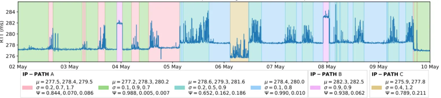
02 May 03 May 04 May 05 May 06 May 07 May 08 May 09 May 10 May 276 278 280 282 284 RTT (ms) at-vie-as1120.anchors.atlas.ripe.net vn-sgn-as24176.anchors.atlas.ripe.net IP PATH A = 277.5, 278.4, 279.5 = 0.2, 0.7, 1.7 = 0.844, 0.070, 0.086 = 277.2, 278.3, 280.2 = 0.1, 0.9, 0.7 = 0.988, 0.005, 0.007 = 278.6, 279.3, 281.6 = 0.2, 0.5, 0.9 = 0.652, 0.162, 0.186 = 278.4, 280.0 = 0.1, 0.8 = 0.990, 0.010 IP PATH B = 282.3, 282.5 = 0.9, 0.9 = 0.938, 0.062 IP PATH C = 275.9, 277.8 = 0.4, 1.2 = 0.789, 0.211

Fig. 1. Segmentation of RTT observations between at-vie-as1120 and vn-sgn-as24176 using an HDP-HMM with DP-GMM emissions. Each color identifies a state.

In this work we focus on two usages of Atlas measurements: to validate the obtained segmentation by correlating hidden states with IP paths observed in traceroutes, and to demonstrate the interpretability of the HMM parameters.

1) Correlation between hidden states and IP paths: We hypothesized earlier that the distribution of delay observations is conditioned on the underlying network state, such as the inter and intra-AS routing configuration, as well as the traffic level. If this is the case, we should observe that changes in IP path result in changes in the HDP-HMM hidden state. As we will see the opposite is not necessarily true. For a given IP path different RTT distributions, and thus different hidden states, can be observed due to changes in traffic levels or at a lower layer. In order to study this correlation we rely on Atlas anchoring mesh measurements. These measurements are setup between every anchors pairs in a full-mesh topology and provide ICMP delay measurements every four minutes as well as ICMP traceroute measurements every fifteen minutes, both on forward and reverse paths. Our dataset consists of IPv4 RTT measurements between all Atlas anchors and the at-vie-as1120 anchor, from the 2nd to the 9th of May 2018. Considering the subset of anchors that were online over the time period, we collected 301 series of 2520 data points.

We learned the HDP-HMM model following Section III-E and producing segmentation results such as those of Fig. 1. Using a Julia implementation of the sampler we can infer the parameters of a 2520 points RTT timeseries with 500 iterations of the sampler in less than 5 seconds on a 2.80GHz Intel Core i7-7600U CPU. 40% of the one-week long series had 1 state, 30% 2 states, 12% 3 states, and the remaining 18% less than 11 states. For every observation and its inferred hidden state we then counted how many different IP paths were observed in the corresponding traceroute measurements. As shown in Figure 2, the majority of states learned over all the paths matches only one AS path and one IP path. For example there are 595 states which always correspond to the same AS path over the 746 states learned. Stated differently only 21% of the states learned can match two AS paths or more. States associated with more than one AS path can be explained by delay differences too small to be separated into two clusters.

Conversely one IP or AS path may be associated to more

than one state. In the traceroutes associated to the anchor pairs of Figure 1, only three different IP paths are identified for 6 hidden states (represented by different colors). In this particular case all the IP paths match the same AS path, and all changes occur in the transit provider AS (Cogent, 130.117.0.0/16, 154.54.0.0/16). We observe that new hidden states are learned when the distribution of the delay changes, potentially due to congestion. Being able to detect these events, invisible in traceroutes, allows for more thorough analysis of Internet path performances, as shall be demonstrated in future works.

1 2 3 4 Number of unique AS-level paths 0 200 400 600 Number of states 1 2 3 4 5 6 7 8 Number of unique IP-level paths

Fig. 2. Distribution of the number of states associated with a given number of unique AS and IP-level paths.

2) Interpretation of the model parameters: An advantage of HMMs over other timeseries models (e.g. autoregressive models or neural networks) is that there is a notion of hidden states and the parameters are easily interpretable with respect to the application domain. In our case the transition matrix gives us information about the frequency and the duration of network configuration changes and the relation between them, while the observations distributions gives us in particular the mean value of the delay and its variance in each state.

Figure 1 shows one of the series learned, where each color identifies a state learned by the model and with the corresponding parameters (components means µ, variances σ, and weights Ψ). We can distinguish two types of states: states where the delay stays relatively constant (such as the blue one), and states where the delay experiences high variations (such as the cyan one). This is reflected by the number of

components learned for the mixture model associated to each state, and the standard deviation of the components. Two gaussians are associated to the blue state, one of which has most of the weight (ψ = 0.990) and a small standard deviation (σ = 0.1). Three gaussians with higher standard deviations (σ = 0.2, 0.5, 0.9) are associated to the cyan state. States with a high variance could possibly be explained by intra-domain load-balancing (since Atlas pings flow ID is not constant), congestion, or in-path devices delaying the processing of ICMP packets. However asserting the cause of such variations and studying the possibility of detecting them from delay measurements is to be done in future works.

The average duration spent by a HMM in state i is given by 1/(1 − πii) where πii is the probability of self-transition

for state i. In the example of Figure 1, the average duration of the pink state is 40 timesteps while the average duration of the green state is 100 timesteps (with one timestep being equal to four minutes).

B. Changepoint detection

Detecting significant changes in RTT values over time is of great interest for network management, network reliability, and security. The use of changepoint detection methods allows to filter out temporary delay fluctuations in order to avoid false alarms. In [16] changepoint detection is performed by mini-mizing the objective function Pm+1

i=1 C(y(τi−1+1):τi) + βf (m)

where C is a cost function that measures the stability or unstability of the delay over a range of successive delay values and βf(m) is a penalty to prevent overfitting. In order to evaluate these methods, with various cost functions and penalties, [16] has produced a publicly available human-labelled changepoint dataset. Although changepoint detection is not our primary focus, the existence of a dataset with some groundtruth allows us to evaluate the quality of the segmentation performed by the HDP-HMM.

In [16] several classification performance metrics are computed: the precision # True Positive

# True Positive+# False Positive, the recall # True Positive

# True Positive+# False Negative, and the F2-score 54×Precision+RecallPrecision×Recall .

The weighted F2-score is computed on the weighted recall, which gives more importance to large RTT changes. We have reproduced the results of [16] and compared the segmentation obtained with HDP-HMM to the two best performing methods: a Poisson cost function, and a nonparametric changepoint detection method, both with a MBIC penalty. The labelled dataset contains 50 RTT series of varying lengths for a total of 34,008 hours of observations. We have performed the following steps to detect changes with the HDP-HMM: 1) learn the model, 2) compute the most likely hidden state se-quence, 3) define changepoints as changes in the hidden states sequence. We have computed the classification performance metrics on each series. The cumulative distribution functions of the performance metrics are displayed on Figure 3. While the precision of changepoint detection with HDP-HMM is similar to the two best performing methods of [16], the recall is significantly improved. This means that the model detected more true changes. In other words, our model is more sensitive

to small changes in the delay without generating unnecessary false alarms.

Note that changepoint detection is only one feature made possible by HDP-HMM modelling. The benefits of such an approach go much further than simply detecting changes as it produces a temporal model, that is useful for delays dynamics characterization and prediction, which is not the case of standard changepoint detection methods.

C. Parsimonious monitoring

In comparison to simpler models, such as mixture models, HMMs account for temporal dependencies, and as such allow for prediction. We exploit this ability to reduce the monitoring cost in routing overlays.

Nodes are connected in a full-mesh topology and one seeks to choose the lowest delay path between an origin and a destination. The possible paths between source and destination are monitored in order to evaluate their delay and choose the best path, but the goal is to limit the frequency of measurements. Current approaches use all-pair probing which makes the probing cost prohibitive (O(n2_{)with n, the number}

of nodes).

We have proposed a method to balance the number of measurements with the routing error [17]. This method is based on a Markov modelling of the dynamics of delay on each path. The problem of deciding or not to measure a path and of selecting the ”best” path between source and destination is then represented as a Markov decision process (MDP). Given the current knowledge of paths delays, our method gives which path to monitor, and when.

Interpretation of the parsimonious monitoring problem as a MDP is possible because of the Markov model used for the paths’ delays. The performance of the method strongly depends on the accuracy of the models. Accurate models permit to forecast future delays without constantly probing the path provided the path delays are stable enough. In order to characterize each path’s delay we have used a sticky HDP-HMM model with DPMM emission distributions.

We briefly summarize here the main results obtained, and refer the reader to [17] for more details on the problem formulation and solution. In order to validate our approach, we have simulated an overlay using delay measurements from RIPE Atlas. We have built a 30-nodes topology by choosing five anchors on each of the six continents. For each origin-destination pairs we only retained the two paths (direct or one-hop) which were the shortest most of the time. We then considered the problem of dynamically deciding to monitor or not path A or path B and to route the traffic on the path supposed to be the shortest one.

In Figure 4 we show the average additional delay over the optimal path for different path selection methods. Some path selection methods are static: path A or path B, or the path which is the best one most of the time, are constantly selected to route the traffic. The two methods at the bottom of Figure 4 are dynamic: constantly monitor paths A and B and at each time slot select the shortest path, or use the

0.0 0.25 0.5 0.75 1.0 Precision 0.00 0.25 0.50 0.75 1.00 CDF 0.0 0.25 0.5 0.75 1.0 Recall 0.0 0.25 0.5 0.75 1.0Recall_w 0.0 0.25 0.5 0.75 1.0F2 0.0 0.25 0.5 0.75 1.0F2_w cpt_np&MBIC cpt_poisson&MBIC HDP-HMM

Fig. 3. Comparison of the HDP-HMM with the changepoint detection methods evaluated in [16].

0

5

10

15

20

25

30

Average additional delay over the optimal path (ms)

MDP

Always

measure

Never

measure

Path B

Path A

static path selection

optimized path selection

Fig. 4. Comparison of the average delay for a static path selection and an optimized path selection with different monitoring policies. Box bounds correspond to the 25 and 75th percentile, middle bar is the median, and whiskers indicates min. and max. values.

MDP approach to limit the number of measurements and dynamically decide if path A should be monitored, if path B should be monitored and on which path traffic should be routed. It is clear that dynamically choosing the shortest path leads to a reduction in the average delay over a static path selection. The relatively low median values (3-5 ms) are due to the fact that we choose the two shortest paths for every OD pair. In practice delay differences between the paths may be larger. The three bottom boxes show the simulation results for different monitoring policies. In the MDP policy the average number of measurements is 0.17 (max 0.65) per time slot so 91% lower than the constant cost of 2 for the always measure policy, while the delay achieved is very close to what we get when always measuring, confirming the good fit of the HDP-HMM models to the delay series.

V. CONCLUSION

We’ve shown that the HDP-HMM, a nonparametric Bayesian model, can be used to estimate HMM parameters, including the number of states, from RTT observations. We have checked on real Internet measurements that the states learned map well to AS paths. Such a flexible model enabled us to achieve precise clustering of delay series. It can also be used to forecast delays and limit the monitoring cost in a network management context such as the routing overlay problem taken as an example. Many applications of the model are yet to be explored. Sequential learning may be used to design parsimonious monitoring schemes without the need for historical measurements, and to detect new network states

in real-time (e.g. for incident detection). The hidden state sequences could be used to align different measurements series and detect correlated changes. The model could also be applied to other delay measurements such as DNS response times, and potentially other QoS metrics.

REFERENCES

[1] M. Yang, J. Ru, X. R. Li, H. Chen, and A. Bashi, “Predicting Internet end-to-end delay: a multiple-model approach,” in Proceedings IEEE 24th Annual Joint Conference of the IEEE Computer and Communications Societies., vol. 4, March 2005, pp. 2815–2819 vol. 4.

[2] E. Kamrani, H. R. Momeni, and A. R. Sharafat, “Modeling internet delay dynamics for teleoperation,” in Proceedings of 2005 IEEE Conference on Control Applications, 2005. CCA 2005., Aug 2005, pp. 1528–1533. [3] S. Belhaj and M. Tagina, “Modeling and prediction of the internet end-to-end delay using recurrent neural networks,” Journal of Networks, vol. 4, no. 6, pp. 528–535, 2009.

[4] Y. Sato, S. Ata, I. Oka, and C. Fujiwara, “Using mixed distribution for modeling end-to-end delay characteristics,” 01 2005.

[5] J. A. Hernandez and I. W. Phillips, “Weibull mixture model to charac-terise end-to-end Internet delay at coarse time-scales,” IEE Proceedings - Communications, vol. 153, no. 2, pp. 295–304, April 2006. [6] K. Salamatian and S. Vaton, “Hidden Markov Modeling for Network

Communication Channels,” SIGMETRICS Performance Evaluation Re-view, vol. 29, no. 1, pp. 92–101, Jun. 2001.

[7] W. Wei, B. Wang, and D. Towsley, “Continuous-time hidden Markov models for network performance evaluation,” Performance Evaluation, vol. 49, no. 1, pp. 129 – 146, 2002, performance 2002.

[8] A. Dainotti, A. Pescap´e, P. S. Rossi, F. Palmieri, and G. Ventre, “Internet traffic modeling by means of Hidden Markov Models,” Computer Networks, vol. 52, no. 14, pp. 2645 – 2662, 2008.

[9] R. Fontugne, J. Mazel, and K. Fukuda, “An empirical mixture model for large-scale RTT measurements,” in 2015 IEEE Conference on Computer Communications (INFOCOM), April 2015, pp. 2470–2478.

[10] C. P. Robert and G. Casella, Monte Carlo Statistical Methods. Springer-Verlag, 1998.

[11] T. S. Ferguson, “A Bayesian Analysis of Some Nonparametric Prob-lems,” The Annals of Statistics, vol. 1, no. 2, pp. 209–230, 1973. [12] J. Sethuraman, “A constructive definition of Dirichlet priors,” Statistica

Sinica, vol. 4, pp. 639–650, 1994.

[13] Y. W. Teh, M. I. Jordan, M. J. Beal, and D. M. Blei, “Hierarchical Dirichlet Processes,” Journal of the American Statistical Association, vol. 101, no. 476, pp. 1566–1581, Dec. 2006.

[14] E. B. Fox, E. B. Sudderth, M. I. Jordan, and A. S. Willsky, “A sticky HDP-HMM with application to speaker diarization,” The Annals of Applied Statistics, pp. 1020–1056, 2011.

[15] J. Van Gael, Y. Saatci, Y. W. Teh, and Z. Ghahramani, “Beam sampling for the infinite hidden markov model,” in Proceedings of the 25th International Conference on Machine Learning, ser. ICML ’08. New York, NY, USA: ACM, 2008, pp. 1088–1095.

[16] W. Shao, J. L. Rougier, A. Paris, F. Devienne, and M. Viste, “One-to-One Matching of RTT and Path Changes,” in 2017 29th International Teletraffic Congress (ITC 29), vol. 1, Sept 2017, pp. 196–204. [17] S. Vaton, O. Brun, M. Mouchet, P. Belzarena, I. Amigo, B. J. Prabhu,

and T. Chonavel, “Joint minimization of monitoring cost and delay in overlay networks: optimal policies with a Markovian approach,” Journal of Network and Systems Management, 2018.