HAL Id: hal-01689868
https://hal.inria.fr/hal-01689868
Submitted on 22 Jan 2018
HAL is a multi-disciplinary open access
archive for the deposit and dissemination of
sci-entific research documents, whether they are
pub-lished or not. The documents may come from
teaching and research institutions in France or
abroad, or from public or private research centers.
L’archive ouverte pluridisciplinaire HAL, est
destinée au dépôt et à la diffusion de documents
scientifiques de niveau recherche, publiés ou non,
émanant des établissements d’enseignement et de
recherche français ou étrangers, des laboratoires
publics ou privés.
Efficient Decentralized Collaborative Mapping for
Outdoor Environments
Luis Contreras-Samamé, Olivier Kermorgant, Philippe Martinet
To cite this version:
Luis Contreras-Samamé, Olivier Kermorgant, Philippe Martinet. Efficient Decentralized Collaborative
Mapping for Outdoor Environments. International Conference on Robotic Computing, Jan 2018,
Laguna Hills, United States. �hal-01689868�
Efficient Decentralized Collaborative Mapping for Outdoor
Environments
Luis Contreras, Olivier Kermorgant and Philippe Martinet
Abstract—An efficient mapping in mobile robotics may involve the participation of several agents. In this context, this article presents a framework for collaborative mapping applied to outdoor environments considering a decentralized approach. The mapping approach uses range measurements from a 3D lidar moving in six degrees of freedom. For that case, each robot performs a local SLAM. The maps are then merged when communication is available between the mobile units. This allows building a global map and to improve the state estimation of each agent. Experimental results are presented, where partial maps of the same environment are aligned and merged coherently in spite of the noise from the lidar measurement.
I. INTRODUCTION
In the area of mobile robots, many tasks are related with exploration and re-construction of the environments. These tasks involve problems as Simultaneous Localization and Mapping (SLAM), in which the mobile robot is placed in an unknown environment and must estimate the map of its surroundings as well as its pose (position and orientation) relative to the map. This is a complex task since determining the robot’s localization typically requires prior knowledge of its surroundings, and on the other hand, map building of its surroundings requires knowledge of the robot’s localization. In order to build a map, the robot has to traverse the unknown environment and incrementally collect measurements of its surroundings and new pose. Furthermore, the presence of uncertainty and noise in the measurements from the sensors, produces accumulate errors over time that consequently distort the robots estimate of its position and map.
The mapping of a large area may require the use of a group of robots that build the maps in a reasonable amount of time considering accuracy in the map construction [1]. So, a set of robots extends the capability of a single robot by merging measurements from group members, providing each robot with information beyond their individual sensors range. This allows a better usage of resources and executes tasks which are not feasible by a single robot. Multi-robot mapping is considered as a decentralized approach when each robot builds their local maps independently of one another and merges their maps upon rendezvous. On the other hand, a centralized approach would require all data to be merged at a single computation unit.
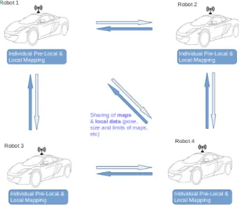
The proposal of this article is a collaborative decentralized mapping framework for efficient merging of 3D maps (see Figure 1 ) where:
• In the first stage named “Pre-Local Mapping”, each
indi-vidual robot builds its map and sends a certain part of it to The authors are from the Laboratoire des Sciences du Num´erique
de Nantes (LS2N), Ecole Centrale de Nantes (ECN), France.
Emails: {Luis.Contreras, Olivier.Kermorgant,
Philippe.Martinet}@ls2n.fr
This article is based upon work supported by the Sustain-T Erasmus Mundus Project.
Fig. 1. Architecture of our Collaborative Decentralized Mapping System
the other robots based on our proposed Sharing algorithm. Low-cost GPS data is used for the first alignment between maps represented in a global frame.
• For the second stage named “Local Mapping”, the
reg-istration process considers the first alignment previously mentioned and includes an intersecting technique of maps to reduce the required bandwidth.
This article is organized as follows: Section II presents
the current works developed in this field. We then detail our
approach in Section III. Finally, experimental results are
presented and analyzed in Section IV, from data acquired on the campus of cole Centrale de Nantes.
II. RELATED WORKS
One of the topic to consider in mapping is the type of sensor used in the robot navigation. In this context, lidar has become a useful range sensor for these applications [2] [3]. Nonetheless, when the lidar scan rate is higher than its tracking, distortion may occur in the map building. In this case, standard registration methods as ICP [4] can be applied to match laser returns for different scans.
Bosse and Zlot [5] [6] [7] use a 2-axis lidar and matches geometric structures of a set local point generated by the lidar in order to build a point cloud [7]. The mapping system includes an IMU and uses loop closure to reconstruct large maps. This approach is based on batch processing to build maps with accuracy and hence is not applicable to real-time mapping.
In the proposed approach, we consider a Pre-Local Mapping stage, which extracts and matches geometric features in
Carte-sian space based on [8]. Our system uses these pre-local clouds inside a more global (at least 2 maps) registration process, ensuring both computation speed and accuracy.
The map representation is crucial when merging and com-munication are considered. Occupancy grids and feature maps are popular approaches in this domain [9]. In this context, in [10], the authors presented method for 3D merging of occupancy grid maps based on octrees [11], [12], [13], [14], [15], [16]. The corresponding experiments consisted in using two simulated robots that traverse an simulated environment and take sensor observations about the scenario for the maps construction. These maps are stored in files and finally merged offline. Furthermore, an accurate transformation between maps was supposed being known, however in real applications, the transform matrix between two robots map is usually only coarsely estimation from sensor observations.
This work was extended in [17], where the subset of points included in the common region is extracted prior to the merge. Then, the merging process refines the transformation estimate between maps by ICP registration [4]
In this paper, we assume two types of environment repre-sentation during the process: 3D point clouds format for the local stage and grid representation for the global one. We also consider a technique to exchange maps between robots while optimizing the registration step. The overall method is part of the decentralized paradigm, where map merging is executed in different units while traversing the environment. In order to ensure communication range, we consider a meeting point for the vehicles in order to exchange their maps and other data [18].
We now present an overview of our contribution.
III. METHODOLOGY
In this section the general overview of the approach is first described. We then focus on each of the stages leading to merged maps for each vehicles according to their communi-cation capabilities.
A. Overview
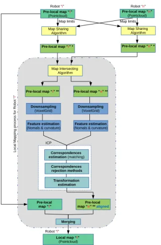
Figure 2 describes the general scheme of our collaborative mapping system implemented on a robot. Each mobile robot executes the mapping task using its on-board lidar sensor and computer. In the beginning, each vehicle independently esti-mates the 3D-map of the environment using a method based on the LOAM (Lidar Odometry And Mapping) technique [8], [19]. This method constructs an environment map represented in the respective local coordinate systems of each vehicle using range measurements from a 3D lidar moving in 6-DOF. Then all the robots use a common reference frame for their maps, where the absolute pose information for each robot is provided by GPS prior to the map construction. All this first stage is indicated as Pre-Local Mapping and those initial maps in point cloud format are denoted as Pre-Local maps.
Afterwards all the vehicles send information about its Pre-Local maps (as bounding cubic lattice of the point cloud) to a Sharing Algorithm, which processes that data for then deciding what part of the Pre-Local map is sent to another robot.
For the next stage, indicated as the Local Mapping, it is necessary for robots to merge the resultant Pre-Local maps into one large and new Local map. During this registration
Pre-local map “i” *
Robot “i”
Downsampling
(VoxelGrid)
Feature estimation
(Nomals & curvature)
Pre-local map “n” *
Downsampling
(VoxelGrid)
Feature estimation
(Nomals & curvature)
Correspondences estimation (matching) Correspondences rejection methods Transformation estimation ICP
Pre-local map “i” ** Pre-local map “n” **
Pre-local
map “i” map “Pre-local n” ** aligned
Map Intersecting Algorithm Merging Local map “i” (Pointcloud) L o ca l M a p p in g p ro ce ss f o r R o b o t “ i ” Robot “i” Map Sharing Algorithm Pre-local map “i” (Pointcloud) Robot “n” Map Sharing Algorithm Pre-local map “n” (Pointcloud)
* Certain part of the Pre-Local Map after Map Sharing Algorithm
** Certain part of the Pre-Local Map* after Map Intersecting Algorithm
Map limits Map limits
Fig. 2. System Architecture for one robot
process, a Map Intersecting Algorithm is executed to extract the intersecting volumes from each map. Finally, a refinement for maps alignment is performed by an Iterative Closest Point (ICP) algorithm, which leads to a consistent local map.
We now detail each mentioned stages. B. Pre-Local Mapping Stage
As previously mentioned, each mobile robot executes a Pre-Local Mapping system based on the LOAM method [8] using as devices a computer and a lidar sensor.
Fig. 3. Architecture of Pre-Local Mapping Stage based on [8]
Figure 3 illustrates the block diagram of this stage, where ˆP
is the generated point cloud. For each sweep, ˆPis registered
in the lidar coordinates {L}. The combined point cloud during
each sweep k generates Pk. This Pk is processed by an
algorithm named Lidar Odometry, which runs at a frequency around 10Hz and receives this point cloud and computes
the lidar motion (transform Tk) between two consecutive
lidar motion. The resultant undistorted Pk is processed at a frequency of 1Hz by performing the matching and registration of the undistorted cloud onto a map. Finally, using the GPS in-formation of the vehicle pose during, it is possible to coarsely project the map of each robot into a common coordinate frame for all the robots. This projected cloud is denoted as the Pre-Local Map.
We now detail the lidar odometry and mapping scheme that is used to build the local map of each robot.
1) Lidar Odometry: Lidar odometry is based on feature
points extraction from the point cloud. The feature points are selected for sharp edges and planar surface patches. For that, we consider that S is the set of consecutive points i returned by
the laser scanner in the same scan, where i ∈ Pk. An indicator
to evaluate the smoothness of the local surface is defined as:
c = 1 | S | . k XL (k,i)k k X j∈S,j6=i (X(k,i)L − X(k,j)L ) k, (1)
where X(k,i)L and X(k,j)L are the coordinates of two points from
the set S.
Moreover, a scan is split into four subregions to uniformly distribute the selected feature points within the environment. The criteria to select the feature points as edge points is related to maximum c values, and by contrast the planar points selection to minimum c values. When a point is selected, it is thus mandatory that none of its surrounding point are already selected, the other conditions being that selected points on a surface patch can not be approximately parallel to the laser beam, or on boundary of an occluded region.
When the correspondences of the feature points are found based on the method proposed in [8], then the distances from a feature point to its correspondence are computed. The min-imization of the overall distances of the feature points allows to obtain the so-called lidar odometry. That motion estimation is modeled with constant angular and linear velocities during a sweep.
Let us define Ek+1 and Hk+1 as the sets of edge points
and planar points extracted from Pk+1, for a sweep k + 1. The
lidar odometry relies on establishing a geometric relationship
between an edge point in Ek+1 and the corresponding edge
line:
fE(X(k+1,i)L , T L
k+1) = dE, i ∈ Ek+1, (2)
where Tk+1L is the lidar pose transform between the starting
time of sweep k + 1 and the current time t. Tk+1L contains
information about the sensor rigid motion in 6-DOF, Tk+1L =
[tx, ty, tz, θx, θy, θz]T, in which tx, ty, and tz are translations
along the axes x, y, and z from {L}, respectively, and θx, θy,
and θz are rotation angles, following the right-hand rule.
Similarly, the relationship between an planar point in Hk+1
and the corresponding planar patch is: fH(X(k+1,i)L , T
L
k+1) = dH, i ∈ Hk+1, (3)
Equations (2) and (3) can be reduced to a general case for
each feature point in Ek+1 and Hk+1, obtaining a nonlinear
function, as:
f (Tk+1L ) = d, (4)
in which each row of f is related to a feature point, and d possesses the corresponding distances. The Levenberg-Marquardt method [20] is used to solve Equation (4). For
that case, the Jacobian matrix (J) of f with respect to Tk+1L
is computed. Then, the minimization of d through nonlinear iterations allows to solve the sensor motion estimation,
Tk+1L ←− Tk+1L − (J
T
J + λdiag(JTJ))−1JTd, (5)
where λ is the Levenberg-Marquardt gain.
Finally, the Lidar Odometry algorithm produces a pose
transform TL
k+1 that contains the lidar tracking during the
sweep between [tk+1, tk+2] and simultaneously a undistorted
point cloud ¯Pk+1. Both outputs will be used by the Lidar
Mappingalgorithm, detailed in the next section.
2) Lidar Mapping: This algorithm is used only once per
sweep and runs at a lower frequency (1Hz) than the Lidar
Odometryalgorithm (10Hz). The technique matches, registers
and projects ¯Pk+1 (provided by the the Lidar Odometry
algorithm) as a map into the own coordinates system of the vehicle “i” {V i}. To understand the technique behavior, let us
define Qk as the point cloud accumulated until sweep k, and
TkV i as the sensor pose on the map at the end of sweep k,
tk+1. The algorithm extends TkV i for one sweep from tk+1to
tk+2, to get Tk+1V i , and projects ¯Pk+1on the robot coordinates
system {V i}, denoted as ¯Qk+1. Then, by optimizing the lidar
pose TV i
k+1, the matching of ¯Qk+1with Qk can be obtained.
In this step the feature points extraction and the finding feature points correspondences are computed in the same way as in previous step (Lidar odometry), the difference just lies
in that all points in ¯Qk+1 share the time stamp, tk+2.
In that case, the nonlinear optimization is solved also by
the Levenberg-Marquardt method, registering ¯Qk+1 on the a
new accumulated map. To get a points uniform distribution, down-sampling process is performed to the map cloud using a voxel grid filter [21] with a voxel size of 5cm cubes. Finally, since we have to work with multiple robots, we use a common coordinates system for their maps, {W }, coming from rough GPS position estimation.
We now present the map sharing stage, happening when two robots are in communication range.
C. Map Sharing Stage
After the generation of Pre-Local Maps, the robots would have to exchange their maps to start the maps alignment process. In several cases the sharing and processing of maps of large dimensions can limit negatively the performance of the system with respect to runtime and memory usage. A sharing technique is presented in order to overcome this problem, in which each vehicle builds only sends a certain part of its map to the other robots.
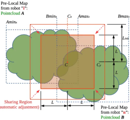
Figure 4 depicts the behavior of the proposed method, in which point clouds A and B represent the Pre-Local Maps from two different robots “i” and “n” respectively. In each robot the algorithm first receives only information about the 3D limits of the maps (i.e. bounding cubic lattice of the point clouds) and then decides what part of its map will be shared to the other robot.
Algorithm 1 presents the pseudo-code of the map sharing initial stage. This function sorts in ascending order the array
Pre-Local Map from robot ”i”: Pointcloud A
Pre-Local Map from robot ”i”: Pointcloud A Pre-Local Map from robot ”n”: Pointcloud B Pre-Local Map from robot ”n”: Pointcloud B Sharing Region (automatic adjustment)Sharing Region (automatic adjustment) Aminx Aminx Amaxx Amaxx Bminx
Bminx CCxx BmaxBmaxxx
Cy Cy C C L L L L L L LL Linit Linit
Fig. 4. Graphical representation of the Map Sharing technique (Top view of plane xy). Ax−min, Ax−max, Bx−minand Bx−maxrepresent the point cloud limits along the x-axis
Data: Point Cloud A, Vectors Amin, Amax, Bmin and
Bmax, Scalars Linit, Lstep, N pmax
Result: Point Cloud Asel
begin
Asel ← ∅;
Cx = 0; Cy = 0; Cz = 0;
(V 2x, V 3x) =
GetV alues(Aminx, Amaxx, Bminx, Bmaxx);
(V 2y, V 3y) =
GetV alues(Aminy, Amaxy, Bminy, Bmaxy);
(V 2z, V 3z) =
GetV alues(Aminz, Amaxz, Bminz, Bmaxz);
Cx = (V 2x+ V 3x)/2;
Cy = (V 2y+ V 3y)/2;
Cz = (V 2z+ V 3z)/2;
N p = P ointSize(A);
for (L=Linit ; N p > N pmax ;L = L - Lstep)do
Sminx= Cx− L ; Smaxx = Cx+ L;
Sminy = Cy− L ; Smaxy = Cy+ L;
Sminz = Cz− L ; Smaxz = Cz+ L;
foreach a ∈ A do if Sminx < ax< Smaxx
and Sminy < ay < Smaxy andSminz < az <
Smaxz then Asel= Asel+ a; end N p = P ointSize(Asel); end end
Algorithm 1: Selection of Point Cloud to share with another robot
of components along each axis of the vectors Amin, Amax, Bmin, Bmax and returns the 2nd and 3rd values from this sorted array, denoted (V 2) and (V 3) respectively. Next, for each axis, the average of the two values obtained by the function GetV alues() is used in order to determine the
Cartesian coordinates (Cx,Cy,Cz) of the geometric center of
the sharing region.
This map sharing region is a cube whose edge length 2L is determined iteratively. Actually, the points from A contained
in this cube region are extracted to generate a new point
cloud Asel. In each iteration the cube region is reduced until
the number of points from Asel is smaller than the manual
parameter N pmax, which represents the number of points
maximum that the user wants to exchange between robots.
Once the loop ends, Asel is sent to the other robot. Similarly
on the other robotic platform “n”, the points from B included
in this region are also extracted to obtain and share Bsel with
the another robot “i”.
We now focus on the local mapping, that is the map merging on a given mobile unit.
D. Local Mapping Stage
In this section the Local Mapping is detailed, considering that the process is executed on the robot “i” with a shared map coming from robot “n”.
1) Preparation for Registration step: The computed
inter-secting volume of the two maps Asel and Bsel is denoted
Aint and Bint and can be obtained from the exchanged map
bounds [17]. In order to improve the computation speed, point
clouds Aintto Bintfirst go through a down-sampling process
in order to reduce the number of points to align of our clouds. The chosen voxel size is 3.5 m cubes in our experimentation. The next step is the feature descriptors estimation, where are computed the surface normals and curvature of the input clouds. This information highly improves the feature points matching, which is the most expensive stage of the ICP algorithm [22]. The normal-point clouds generated after this
step are denominated as AintN and BintN. Those normal point
clouds are then used and aligned in the next step.
2) Registration step with ICP: Environment data used in
this work are aligned with Iterative Closest Point (ICP) algo-rithm [23]. The algoalgo-rithm refines an initial alignment between clouds, which basically consists in estimating the best
transfor-mation to align a source cloud BintN) to a target cloud AintN
by iterative minimization of an error metric function. At each iteration, the algorithm determines the corresponding pairs
(b0,a0), which are the points from AintN BintN respectively
with the least Euclidean distance.
Then, least squares registration is computed and the mean squared distance E is minimized with regards to estimated translation t and rotation R:
E(R, t) = 1 Nb0 Nb0 X i=1 k a’i− (R b’i+ t) k 2 , (6)
The resultant rotation matrix and translation vector can be express in a homogeneous coordinates representation (4×4
transformation matrix Tj) and are applied to BintN. The
algorithm then re-computes matches between points from
AintN and BintN, until the variation of mean square error
between iterations is less than an defined threshold. The final ICP refinement for n iterations can be obtained by multiplying
the individual transformations: TICP = Q
n
j=1Tj. Finally the
transformation TICP is applied to the point cloud Bselto align
and merge with the original point cloud A. Each robot thus performed its own merging according to limited data shared from other agents within communication range.
We now present the experimental results to illustrate the proposed method.
IV. RESULTS
In this section we present results validating the presented concepts and the functionality of the system. As we consider ground vehicles, the ENU(East-North-Up)-coordinate system is used as external reference of the world frame {W }, where y-axis corresponds to North and the scene x-y-axis corresponds to East, but coinciding at the initial position the GPS coordinates [Longitude: -1.547963, Latitude: 47.250229]. The experiments
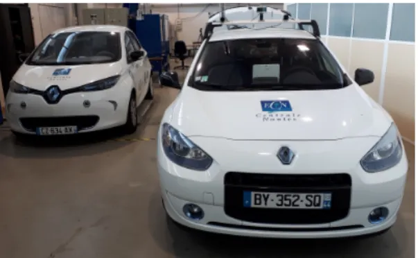
Fig. 5. Vehicles used during the tests
were performed using two vehicles, a Renault Fluence and a Renault Zoe (see Figure 5) customized and equipped with
a Velodyne VLP-16 3D lidar, with 360◦ horizontal field of
view and a 30◦ vertical field of view. All data come from
the campus outdoor environment in an area of approximately 290m x 170m. The vehicles traversed that environment follow-ing different paths and collected sensor observations about the world, running the real-time mapping process on two laptops Core-i5 independently on each vehicle.
Fig. 6. Paths followed during the test (top view). Image source: Google Earth
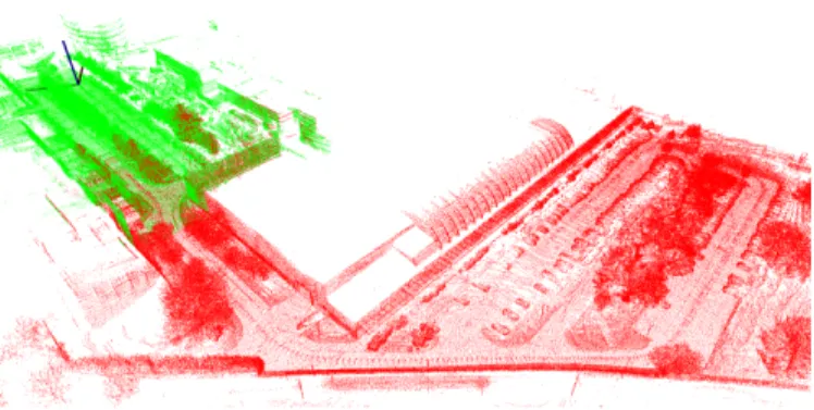
In this experiment the vehicles build clouds (green and red) from different paths (see Figure 6). The results of the Pre-Local Mapping of this experiment are shown in Figure 7. The map of the first robot is shown in green, and in red for the second robot.. Figure 7 depicts the “sharing region” from 2nd robot to 1st robot and the “intersecting region” determined during the alignment process in the 2nd vehicle. For that test, the number of points maximum to exchange
between robots, N pmax, was set to 156000 points. Once the
Sharing stage ends, the systems of each robot performs ICP transform refinement to obtain an improved transform between each map. Figures 8 and 9 depict the Pre-Local point clouds
Fig. 7. Pre-Local Maps for 1st robot (green one) and 2nd robot (red one) projected in common coordinates system prior to ICP refinement. Sharing and alignment region in 2nd robot (top view)
during the alignment process in each robot. Once the refined transformation is obtained, it is then applied to the second map, resulting in merged maps.
(a) (b)
Fig. 8. Alignment of maps with ICP refinement in 1st robot (a) Green and red maps represent the target and source clouds pre ICP, top view (b) Green and blue maps represent the target and aligned source clouds post ICP, top view
(a) (b)
Fig. 9. Alignment of maps with ICP refinement in 2nd robot (a) Green and red maps represent the target and source clouds pre ICP, top view (b) Green and blue maps represent the target and aligned source clouds post ICP, top view
Quantitative alignment results of the ICP are shown in Table I. On the 1st robot the algorithm converged to the value of displacement of 0.693 m and 1.572 m along the x-axis and y-axis respectively. On the other hand on the 2nd robot, the algorithm converged to a value of displacement of -1.110 m and -1.557 m along the x-axis and y-axis respectively. Those
results reconfirm the alignments on opposite directions for both robots, since we must consider that each robot performs a relative registration process considering its Pre-Local map as target cloud for alignment reference.
TABLE I
REFINEMENT TRANSFORMATION MATRICES
Figure 10 shows the results of the final merging in the 1st robot, in which the red map corresponds to the Pre-Local shared by the 2nd robot already aligned to the green map, that represents the Pre-Local map from 1st robot. The fusion of these maps generates the Local Map in the 1st robot. The
Fig. 10. 3D-Map merging result in 1st robot (different view) experiments showed also the importance of selection of maps intersecting region for the alignment, avoiding the divergence of the registration algorithm. Our proposed maps sharing tech-nique develops a transcendental position in the performance of the entire mapping collaborative system. Finally, the sharing algorithm remains a suitable candidate to exchange efficiently maps between vehicles considering the use of maps of the large dimensions.
V. CONCLUSION ANDFUTURE WORK
We presented a framework for decentralized mapping sys-tem for mobile robots. The work has demonstrated that maps from different robots can be successfully merged, from a coarse GPS initial registration to assess the initial intersecting volume. The system uses range measurements from a 3D lidar, generating a local map for each robot. The complete system solves the mapping problem in an efficient way that runs individually online on computers on-board two vehicles for preliminary experiments.
Online tests have been performed on two cars, leading to merged maps on each vehicle. Future works will consider heterogeneous vehicles, such as a fleet of ground and aerial robots where the view points are less similar and where both communication and computing capabilities are a crucial aspect of the whole process.
REFERENCES
[1] P. Dinnissen, S. N. Givigi, and H. M. Schwartz, “Map merging of multi-robot slam using reinforcement learning.” in SMC. IEEE, 2012. [Online]. Available: http://dblp.uni-trier.de/db/conf/smc/smc2012.html# DinnissenGS12
[2] A. N¨uchter, K. Lingemann, J. Hertzberg, and H. Surmann, “6D SLAM - 3d mapping outdoor environments: Research articles,” J. Field Robot., Aug. 2007. [Online]. Available: http://dx.doi.org/10.1002/rob.v24:8/9 [3] S. Kohlbrecher, O. V. Stryk, T. U. Darmstadt, J. Meyer, and U. Klingauf,
“A flexible and scalable SLAM system with full 3d motion estimation,” in in International Symposium on Safety, Security, and Rescue Robotics. IEEE, 2011.
[4] F. Pomerleau, F. Colas, R. Siegwart, and S. Magnenat, “Comparing ICP variants on real-world data sets - open-source library and experimental protocol.” Auton. Robots, 2013. [Online]. Available: http://dblp.uni-trier. de/db/journals/arobots/arobots34.html#PomerleauCSM13
[5] R. Zlot and M. Bosse, “Efficient large-scale 3d mobile mapping and surface reconstruction of an underground mine.” in FSR, ser. Springer Tracts in Advanced Robotics, K. Yoshida and S. Tadokoro, Eds. Springer, 2012. [Online]. Available: http://dblp.uni-trier.de/db/conf/fsr/ fsr2012.html#ZlotB12
[6] M. Bosse, R. Zlot, and P. Flick, “Zebedee: Design of a spring-mounted 3-d range sensor with application to mobile mapping,” IEEE Transactions on Robotics, Oct 2012.
[7] M. Bosse and R. Zlot, “Continuous 3d scan-matching with a spinning 2d laser,” in 2009 IEEE International Conference on Robotics and Automation, May 2009.
[8] J. Zhang and S. Singh, “Loam: Lidar odometry and mapping in real-time,” in Robotics: Science and Systems, 2014.
[9] M. Montemerlo, S. Thrun, D. Koller, and B. Wegbreit, “Fastslam 2.0: An improved particle filtering algorithm for simultaneous localization and mapping that provably converges,” in In Proc. of the Int. Conf. on Artificial Intelligence (IJCAI, 2003.
[10] J. Jessup, S. N. Givigi, and A. Beaulieu, “Merging of octree based 3d occupancy grid maps,” in 2014 IEEE International Systems Conference Proceedings, March 2014.
[11] P. Payeur, P. Hebert, D. Laurendeau, and C. M. Gosselin, “Probabilistic octree modeling of a 3d dynamic environment,” in Proceedings of International Conference on Robotics and Automation, Apr 1997. [12] J. Fournier, B. Ricard, and D. Laurendeau, “Mapping and exploration
of complex environments using persistent 3d model,” Fourth Canadian Conference on Computer and Robot Vision (CRV ’07), 2007. [13] K. Pathak, A. Birk, S. Schwertfeger, and J. Poppinga, “3d forward
sensor modeling and application to occupancy grid based sensor fusion,” in International Conference on Intelligent Robots and Systems (IROS), IEEE Press. IEEE Press, 2007.
[14] N. Fairfield, G. Kantor, and D. Wettergreen, “Real-time slam with octree evidence grids for exploration in underwater tunnels,” J. Field Robotics, 2007.
[15] A. Hornung, K. M. Wurm, M. Bennewitz, C. Stachniss, and W. Burgard, “Octomap: An efficient probabilistic 3d mapping framework based on octrees,” Auton. Robots, Apr. 2013. [Online]. Available: http://dx.doi.org/10.1007/s10514-012-9321-0
[16] A. Hornung, K. M. Wurm, and M. Bennewitz, “Humanoid robot localization in complex indoor environments,” in 2010 IEEE/RSJ In-ternational Conference on Intelligent Robots and Systems, Oct 2010. [17] J. Jessup, S. N. Givigi, and A. Beaulieu, “Robust and efficient multirobot
3-d mapping merging with octree-based occupancy grids,” IEEE Systems Journal, 2015.
[18] N. E. ¨Ozkucur and H. L. Akin, “Supervised feature type selection for topological mapping in indoor environments,” in 21st Signal Processing and Communications Applications Conference, SIU 2013, Haspolat, Turkey, April 24-26, 2013, 2013, pp. 1–4. [Online]. Available: http://dx.doi.org/10.1109/SIU.2013.6531556
[19] J. Zhang and S. Singh, “Visual-lidar odometry and mapping: low-drift, robust, and fast,” in 2015 IEEE International Conference on Robotics and Automation (ICRA), May 2015.
[20] R. I. Hartley and A. Zisserman, Multiple View Geometry in Computer Vision, 2nd ed. Cambridge University Press, ISBN: 0521540518, 2004. [21] R. Rusu and S. Cousins, “3d is here: Point cloud library (pcl),” in Robotics and Automation (ICRA), 2011 IEEE International Conference on, May 2011.
[22] S. Rusinkiewicz and M. Levoy, “Efficient variants of the ICP algorithm,” in Third International Conference on 3D Digital Imaging and Modeling (3DIM), Jun. 2001.
[23] P. J. Besl and N. D. McKay, “A method for registration of 3-d shapes,” IEEE Trans. Pattern Anal. Mach. Intell., Feb. 1992. [Online]. Available: http://dx.doi.org/10.1109/34.121791