HAL Id: hal-02337955
https://hal.archives-ouvertes.fr/hal-02337955
Submitted on 29 Oct 2019
HAL is a multi-disciplinary open access
archive for the deposit and dissemination of
sci-entific research documents, whether they are
pub-lished or not. The documents may come from
teaching and research institutions in France or
abroad, or from public or private research centers.
L’archive ouverte pluridisciplinaire HAL, est
destinée au dépôt et à la diffusion de documents
scientifiques de niveau recherche, publiés ou non,
émanant des établissements d’enseignement et de
recherche français ou étrangers, des laboratoires
publics ou privés.
Distributed modeling approach of discrete
manufacturing systems by Parts of Plant
Alexandre Philippot, M Sayed Mouchaweh, Véronique Carré-Ménétrier
To cite this version:
Alexandre Philippot, M Sayed Mouchaweh, Véronique Carré-Ménétrier. Distributed modeling
ap-proach of discrete manufacturing systems by Parts of Plant. 2009 European Control Conference
(ECC), Aug 2009, Budapest, Hungary. �hal-02337955�
Article · March 2015 CITATIONS 0 READS 32 3 authors:
Some of the authors of this publication are also working on these related projects:
Intelligent diagnosisView project
high machining processView project Alexandre Philippot
Université de Reims Champagne-Ardenne 79 PUBLICATIONS 202 CITATIONS
SEE PROFILE
M. Sayed Mouchaweh Institut Mines-Télécom Lille Douai 128 PUBLICATIONS 827 CITATIONS
SEE PROFILE
Véronique Carré-Ménétrier
Université de Reims Champagne-Ardenne 61 PUBLICATIONS 236 CITATIONS
SEE PROFILE
All content following this page was uploaded by Alexandre Philippot on 30 June 2016.
Abstract—The paper presents an original approach to model a discrete manufacturing system by Parts of Plant (PoP). This approach takes into account technical and technological specifications of each plant elements. The aim of this works is to realize a reliable simulation of discrete manufacturing systems in design stage before production stage. Models are distributed and established from the functional chain of a process. They take into account the distribution of information through each PoP with its sensors, pre-actuators and actuators. A PoP library is proposed with their corresponding model. An application example is used to illustrate the approach.
I. INTRODUCTION
simulation is the execution of a model, represented by a computer program that gives information about the dynamic behavior of a system being investigated. This simulation allows evaluating system performances at the design stage. Hence, the latter becomes more flexible and convenience to obtain a more reliable system fulfilling the desired objectives. The simulation stage is based on the use of a model of the system. The model construction depends on several factors as the level of modeling and desired objective: analysis [1], [2], synthesis [3], [4], verification [5], [6], diagnosis [7], [8] or simulation [9].
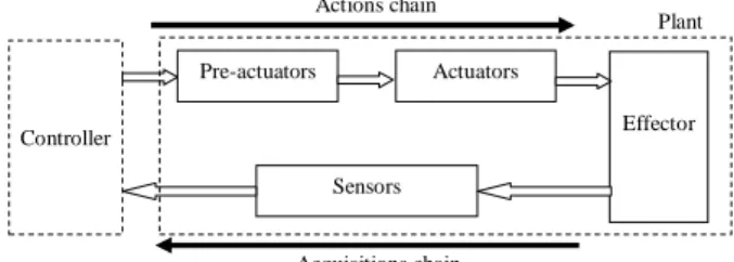
Manufacturing systems can be represented as Discrete Event Systems (DES) [10]. They are composed of elements called “Part of Plant” (PoP). Each PoP can be modeled thanks to its states and its events. Generally, plant is composed of pre-actuators, actuators and sensors (Fig. 1). Each plant component is also divided in sub-components characterized by the technology used to produce them [11]. This division implicates a modular modeling where each sub-component is a PoP. However, in literature, plant is often modeled as a set of “pre-actuators / “pre-actuators / sensors”. These models are often an abstraction of the behavior according to the modeling objectives. For example, a pneumatic cylinder can be modeled as an automatonwith 4 states in verification [5], with 12 states in synthesis [3] or with 18 states in analysis [9].
A. Philippot is with the Centre de Recherche en STIC, Moulin de la Housse, 51687 REIMS, University of Reims, France (corresponding author to provide phone: +33 326-918-616; fax: +33 326-913-106; e-mail: alexandre.philippot@univ-reims.fr).
M. Sayed-Mouchaweh is with the Centre de Recherche en STIC, Moulin de la Housse, 51687 REIMS, University of Reims, France (e-mail: moamar.sayed-mouchaweh@univ-reims.fr).
V. Carré-Ménétrier is with the Centre de Recherche en STIC, Moulin de la Housse, 51687 REIMS, University of Reims, France (e-mail: veronique.carre@univ-reims.fr). Effector Actions chain Acquisitions chain Controller Pre-actuators Actuators Sensors Plant
Fig. 1. Functional line of a process
The aim of this paper is the construction of PoP models for the simulation. These PoP models can be then used for the diagnosis of the system. The basic idea of diagnosis is to collect sequences of observations (or symptoms), in order to decide whether or not a system is working normally (fault detection). Then if a fault is detected, it reports (fault isolation) which fault has occurred (deterministic diagnosis) or the most likely to have occurred (probabilistic diagnosis). Diagnosers are considerate as observers of the behavior and consequently must be re presented by a model.
The interest of the use of PoP is to avoid the combinatory explosion of large DES modeling, [12]. The global model of the system is constructed based on the local models (PoP) which must communicate together. This communication is necessary in order to take into account the interactions among PoP. For that, a protocol (set of rules) is used to define the messages (information) to be exchanged among PoP models. Each PoP model is represented by Moore automata [10]. A Moore automaton is a Finite State Machine (FSM) where the outputs are determined by the current state. To represent the system dynamics evolution, a clock is added to each PoP Moore automaton in order to measure time between events.
The paper is structured as follows. In section 2, a library of the Parts of Plant commonly used in discrete manufacturing systems is presented. In section 3, the models for these different PoP are detailed. These models take into account the technology specifications used to produce them. Then, these models are used through a simulation tool to give information about the dynamic behavior of the system being investigated. An example illustrating these models is found in section 4.
II. PARTSOFPLANTLIBRARY
In manufacturing systems, controller sends commands to the plant to realize actions and receives information about the plant status, in response to these actions, through incoming sensors data. Plant is composed of actions and acquisitions chains (Fig. 1). The actions chain is composed of pre-actuators which
Distributed Modeling Approach of discrete manufacturing systems
by Parts of Plant
A. Philippot, M. Sayed-Mouchaweh and V. Carré-Ménétrier, CReSTIC-URCA
transform the controller commands into power. The latter is then transformed by the actuators into actions realized by the effectors. The acquisitions chain informs the controller about the effectors situation thanks to sensors.
A. Pre-actuators
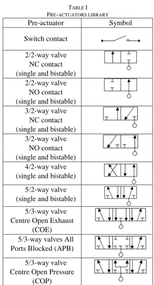
Pre-actuators can be classified in three types: electrics, pneumatics or hydraulics [11]. Electrics pre-actuators are, in most cases, switch contacts or motor controller (e.g. variable-speed drive, regulator…). Switch contacts are discrete and can be open or closed whereas motor controller agrees continuous signals. In the paper, only switch contacts are studied. Readers can found more information on electrics pre-actuators and their symbol in the standard C03-207 of the Technical Union of Electricity (http://www.ute-fr.com/FR/).
Pneumatics valves are pneumatics pre-actuators. They convert pneumatic power in compressed air transmitted to actuators (cylinders). Valves are composed of several exhaust ports and a slide with several positions. The behavior of a valve is characterized by a duo “number of ports/number of positions”. Consequently, a 5/2-way valve, 5 exhaust ports and 2 positions, will have a different behavior of a 2/2-way valve (Fig. 2). Valves can be controlled in single solenoid or bistable. A single valve has only one relax state thanks to a spring whereas bistable valve has two possible relaxes positions according to the last command sent. The control power of pneumatics valves can be electric, pneumatic, mechanic or combined. Another specification, if there is any pressure in relax position, the valve is said to be normally closed (NC). If there is pressure in the valve, then the valve is said to be normally open (NO). All symbols and explanations about pneumatics valves can be found in [11].
Hydraulics valves are also pre-actuators but with hydraulic fluid as power. They are used only with hydraulics actuators and have often the same characteristics as pneumatics valves. Table I enumerates the set of pre-actuators commonly used in a library.
B. Actuators
Actuators are generally divided into three families [11]. The first is the electrics actuators as motors (induction motor, electric stepping motor, DC motor, AC motor,…), as well as solenoid, resistor, etc…. Readers can found more information about electrics actuators and their symbol in the standard C03-207 of the Technical Union of Electricity ( http://www.ute-fr.com/FR/).
2/2-way valve 5/2-way valve
1 3 1
2 2
5 4
Fig. 2. 2/2-way and 5/2-way valves
TABLE I PRE-ACTUATORS LIBRARY Pre-actuator Symbol Switch contact 2/2-way valve NC contact (single and bistable)
2/2-way valve NO contact (single and bistable)
3/2-way valve NC contact (single and bistable)
3/2-way valve NO contact (single and bistable)
4/2-way valve (single and bistable)
5/2-way valve (single and bistable)
5/3-way valve Centre Open Exhaust
(COE) 5/3-way valves All Ports Blocked (APB)
5/3-way valve Centre Open Pressure
(COP)
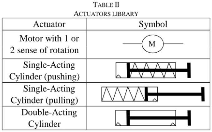
The second family is the pneumatics actuators. The most used ones of this family are the pneumatics cylinders. The latter (sometimes known as air cylinders) are mechanical devices which produce force, often in combination with movement, and are powered by compressed gas (typically air). They convert the potential energy of compressed gas into kinetic energy. They transform pressure in action and force a piston to move in the desired direction, to grow, pull, bend, grip, raise, put together, etc.... Pneumatic cylinders are always associated to one or several pneumatics valves. As the motors, there are many types of pneumatics cylinders as Single-Acting Cylinder (SAC) moving in one direction and Double Acting Cylinders (DAC) moving in both directions. Although SACs and DACs are the most common types of pneumatic cylinders, there exists also rotary air cylinders (actuators that use air to impart a rotary motion), rodless air cylinders (actuators that use a mechanical or magnetic coupling to impart force), etc.
The third type is the hydraulics actuators which produce an important mechanical effort and precision. Hydraulics cylinders are commonly used but in this paper only motors and pneumatics cylinders are studied (Table II).
TABLE II ACTUATORS LIBRARY Actuator Symbol Motor with 1 or 2 sense of rotation M Single-Acting Cylinder (pushing) Single-Acting Cylinder (pulling) Double-Acting Cylinder C. Sensors
Sensors provide information about the response of PoP due to the actuators actions. There are several kinds of sensors as the ones indicating positions (digital sensors) or the ones measuring pressures, temperatures, flow rate, speed ... (analogical sensors). In this paper, we do not treat the analogical sensors but only digital ones with a binary response (active or inactive status) [11]. Sensor’s technology (proximity switch, electro-mechanical, inductive, capacitive, infrared …) has no influence on their functioning.
III. PARTS OF PLANT MODELING
To model each Part of Plant of the libraries (Tables I, II and digital sensors), we have chosen Moore automata. A Moore automaton is a finite state automaton where the outputs are determined by the current state (Fig. 3). It can be defined as a 6-tuple (Q, q0, Σ, Λ, T, G) consisting of the following:
• a finite set of static’s states (Q)
• an initial state x0 which is an element of (Q)
• a finite set of events called the input alphabet (Σ)
• a finite set of events called the output alphabet (Λ)
• a transition function (T : Q × Σ → Q) mapping a state and the input alphabet to the next state
• an output function (G : Q → Λ) mapping each state to the output alphabet
Each PoP is modeled as a block where inputs/outputs must be identified. In this section, a methodology is presented for the definition of each PoP with an example for illustration.
A Moore automaton with x, y, z as inputs and a, b as outputs y b q1 b q3 b q0 a q2 y z z x,y x,z
Fig. 3. A Moore automaton
Pre-actuator
Commands Positions
Fig. 4. Pre-actuator block
A B A C B
pre-actuator 2 positions pre-actuator 3 positions
Fig. 5. Positions of pre-actuator
A. Pre-actuators block
Pre-actuator block receives commands of the controller as input and gives their position in output (Fig. 4). In this paper, we issue assumptions that the displacement from a position to other one is considered as instantaneous. Pre-actuators can take 2 or 3 positions according to their technology. Then, to keep the same notation, we have chooses to define the position of them by letters (Fig. 5). Consequently, left position is always noted by A, right position by B and intermediate position by C. To illustrate our purposes, let us take the case of a 5/2-way bistable valve accepting two commands: Out1 allowing positioning the valve in A and Out2 allowing positioning the valve in B. These 2 positions cannot be simultaneously set to 1. The valve technology makes that the change from a position to other one is instantaneous. There is always only one possible position.
For the modeling, it is necessary to know the valve positions according to all possibilities of inputs. A truth table is established with an expert (Table III). When the command
Out1 is sent alone, then the valve is on position A, and when
the command Out2 is sent alone, then the valve is on position B. However, when Out1 and Out2 are sent or when there is no command, e.g. /Out1./Out2, then the valve keeps the last position. In this case, the last position is memorized and indicated in Table III by the letter “M”. However, at the initialization of the process, it is impossible to know the valve’s position. Consequently, we must add an initial state to the model but without output in order to avoid giving wrong information. Anyway, adding an initial state depends on the pre-actuator technology.
The corresponding model is given in Fig. 6 where, from the initial state q0, the model are waiting for an input information
without “Memory” effect to go to state q1/A or q2/B. The
passage of the state q1/A to the state q2/B is achieved by the
transition /Out1.Out2. The return of the state q2/B towards the
state q1/A is occurred by transition Out1./Out2.
TABLE III
TRUTH TABLE OF 5/2-WAY BISTABLE VALVE MODEL
A B /Out1./Out2 M M Out1./Out2 1 0
Out1.Out2 M M /Out1.Out2 0 1
/Out1.Out2 Out1./Out2 A q1 B q2 Out1./Out2 /Out1.Out2 q0
Fig. 6. 5/2-way bistable valve model
B. Actuators block
Based on Fig. 1, we can note that actuators are preceded by pre-actuators. Thus, actuators block receives the valves positions in its input to provide at its output the actuator functional state (Fig. 7).
Let us take a Double-Acting Cylinder (DAC). This latter is piloted by a pneumatic valve with 2 positions. It accepts the position of this one in input (A or B). In output, the DAC can take 4 states: (i) piston rod back, (ii) piston rod out, (iii) piston rod going back, (iv) piston rod going out. The truth table of the DAC block (Table IV) is provided by an expert. When the valve is in position A, the piston rod of the cylinder must go out. Consequently, the model goes to a dynamic state V->,
marked by a star *. After that, it arrives in a stable state VOUT
where the piston rod is totally out. Conversely, when the valve is in position B, the piston rod comes back and goes to a dynamic state V<- to arrive in a stable state VIN where the
piston rod of the cylinder is totally back. As the pre-actuators blocks, at the initialization state of the process, it is impossible to know if the piston rod of the cylinder is back or totally out. Consequently, we add an initial state to the model without output to avoid giving wrong information.
After the choice of a cylinder type, the dynamic aspect can be established by the time of displacement of the piston rod. This latter needs time to arrive from a stable position to other one. This time is called “Time of stroke” and noted Ts. It
defines of the piston rod stroke s and of the speed v by: Ts = s/v
. However, the speed of a cylinder is a function of the piston rod area A (depending of the piston rod diameter) and of the volumetric rate of the compressed gas R (which is also a function of the presence or not of a pneumatic device like a pressure-reducing valve). Then, the speed is represented by: v = R/A.
Actuator Behaviour of actuator Positions of
pre-actuator
Fig. 7. Actuator block
TABLE IV
TRUTH TABLE OF DAC MODEL
VIN V-> VOUT V
<-A 0 1* 1 0 B 1 0 0 1*
All these technical and technological characteristics are primordial to the modeling. They are often available by the provider in the technical documentation or otherwise can be determined by learning cycles. To integrate this dynamic into models, we have defined a timed Moore automaton where dynamic states are represented by a circle in dotted line. A timed Moore automaton can be defined as a 11-tuple (Q, q0, Σ,
Λ, T, G, Q*, Ts, ∆, t, Ψ) with the 6-tuple (Q, q0, Σ, Λ, T, G) of
a Moore automaton and the following:
• a finite set of dynamic’s states (Q*)
• a Time of stroke (Ts)
• a variable of temporary allocation (∆)
• a local clock between 2 events (t)
• a finite set called operand (Ψ) for allocation (->) and equality test (:=)
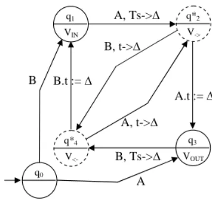
For the DAC example, the model is given in Fig. 8. From the initial state q0 and according to the inputs, the model
evolves towards state q1/VIN or q3/VOUT. From the state q1/VIN,
representing the piston rod in position come back, the cylinder can go out if it accepts position A from the valve. In this transition, the time of stroke Ts is appointed to variable ∆. The
model stays in dynamic state q*2/V-> until the local clock t
becomes equal at the time of stroke. In this case, the model is considered in a state q3/VOUT where the piston rod is out. On
the contrary, if during its exit, the model accepts a new position B from the valve, then the variable ∆ is affected by a new value corresponding to the current time t. The model goes to a dynamic state q*4/V<- where t is re-initialized to 0. The
cylinder goes back to the state q1/VIN at the end of time ∆
defined by the last value of t. The functioning from the state q3/VOUT is similar. As the pre-actuators, the addition of an
initial state depends of its technology.
C. Sensors block
The sensor block broadcasts information on the presence or not of a product or an actuator (Fig. 9). Then, the state of the sensor is sent to the controller. Consequently, the truth table of the sensor model is function of an input E and deducts from it the output state d (Table V). Then, sensor model has only 2 states (Fig. 10). We take the assumption that at the initialization, the sensor is always to 0.
A.t := ∆ A, Ts->∆ B, Ts->∆ B, t->∆ A, t->∆ B.t := ∆ VIN q1 V-> q*2 VOUT q3 V <-q*4 B A q0
Sensor Piece or
actuator Behaviour of
the sensor
E
d
Fig. 9. Sensor block
TABLE V
TRUTH TABLE OF SENSOR MODEL
d /d /E 0 1 E 1 0 /E E d q1 /d q0
Fig. 10. Sensor model
D. Discussion
Two characteristics can only implicate a modification on the model. The first one concerns the piloting in single solenoid or bistable of pre-actuators and the second on the number of positions (2 or 3) which they can take. These two characteristics make possible only 3 different models: (i) single solenoid with 2 positions, (ii) bistable with 2 positions, (iii) bistable with 3 positions (Table VI). The others technological variations, like the number of ports or the fact than a valve is in NO contact or NC contact, don’t change the models structure but can influence on the initial state.
For the actuators library (Table II), it is also possible to consider the same model for several types. Both types of motors, 1 sense and respectively 2 senses of rotation, have different models because they are piloted by 1 or respectively 2 switch contacts. For the cylinders, it is possible to have only one model for SAC or DAC when they have 2 positions because they keep the same type of functioning. The only feature concerns the cylinders piloted by a valve with 3 positions. A new intermediate state is created when the valve is on position C (Table VII).
TABLE VI
LIBRARY OF PRE-ACTUATORS MODELS
Pre-actuator Model Single solenoid /Out1 Out1 A q1 B q0 Bistable with 2 positions /Out1.Out2 Out1./Out2 A q1 B q2 Out1./Out2 /Out1.Out2 q0 Bistable with 3 positions /Out1./Out2 /Out1.Out2 Out1./Out2 /Out1.Out2 Out1./Out2 /Out1./Out2 B q2 A q1 C q0 TABLE VII
LIBRARY OF ACTUATORS MODELS
Actuator Model Motor with 1 sense of rotation C /C Mstop q0 Mrot q1 Motor with 2 sense of rotation C1./C2 /C1./C2 + C1.C2 /C1.C2 /C1./C2 + C1.C2 Mstop q0 M-> q2 M <-q1
SAC and DAC with 2 positions A.t := ∆ A, Ts->∆ B, Ts->∆ B, t->∆ A, t->∆ B.t := ∆ VIN q1 V-> q*2 VOUT q3 V <-q*4 B A q0 DAC with n positions (n>2 and with 5/3-way valve
or equivalent intermediate position C) A.t := ∆ A, Ts->∆ B, Ts->∆ B, t->∆ A, t->∆ B.t := ∆ C C B, Tsint->∆ A, Tsint->∆ VIN q1 V-> q*2 VOUT q3 V <-q*4 Vstop q5 B A C q0
Only digital sensors with a binary response are considered in this paper, and then model of the Fig. 10 is the only one possible.
IV. APPLICATION AND SIMULATION
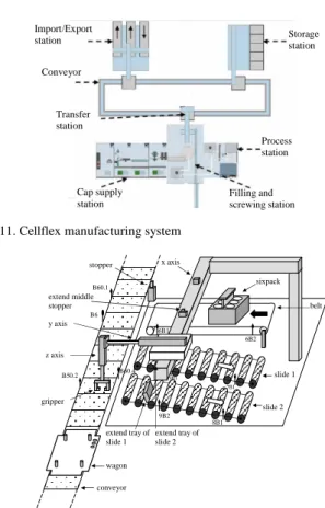
In this section, we present a real flexible manufacturing system cellflex (http://meserp.free.fr/). The task of the system consists in filling bottles to condition them by 6 in a sixpack and finally to stock them. Firstly, the Import/Export station provides sixpacks which are going to be transported from stations to stationsthanks to a central conveyor. Each sixpack is deposited on a wagon. At the same time, the filling station filled the bottles of liquid and deposits a cap there. They are then transported to the transfer station. If a group of six bottles is available, a sixpack is ordered and bottles in wait are put, three in the first line and three in the second line. Then, sixpack returns to the Import/Export station to be put out of the system. If this station is full or blocked, sixpacks is provisionally stocked in the storage station (Fig. 11).
For the moment, the modeling approach by PoP has been realized on the Import/Export station. When a wagon comes front of the import belt, an empty sixpack is put on it thanks to a pneumatic system on 3 axes. After the packaging, the wagon with a full sixpack is situated in front of one of the export
slides. The pneumatic system on 3 axes takes a sixpack and put it on a slide (Fig. 12).
This station is composed of 10 actuators piloted by 12 pre-actuators with different technologies. The information about the behavior of the station is given by 23 sensors. Consequently, all these Parts of Plant can be modeled from our library. These models have been implemented in the software
Stateflow of Matlab® for simulation. Our approach represents 45 local models with a maximum of 6 states and a totality of 127 states (34 states for the pre-actuators, 47 for the actuators and 46 for the sensors). To compare with a global model of this plant, composition operations are need and succeeded to one model with more of 400 states. Consequently, without composition, there is no combinatory explosion in the construction of ours models.
V. CONCLUSIONS AND FUTURE WORKS
This paper presented an original approach to model a plant of manufacturing systems. This modeling is based on distributed information of a plant. We consider that a plant can be divided in several Parts of Plant (PoP) which are different according to the family (pre-actuators, actuators, sensors) and to the specifications (3/2-ways valves, 5/2-ways valves, motors, cylinders…) of their local elements. PoP are modeled by classical and timed Moore automata to allow the communication between models. A library of the commonly used PoP has been established to deduce of it a library of their models.
The first objective of these works is the simulation of systems before production. The distributed modeling introduced in this paper allows validating local Parts of Plant. However, the global behavior of the plant is not validated because it corresponds to correlations between the different local PoP. These correlations are linked to physical constraints of high level which must be also modeled. For example, two cylinders moving in a common area will not have the same global behavior as if they were independent. This problem is a part of ours future works. Another drawback is that there is no product model for the moment whereas this one can influence the process.
To finish, we want to extend ours models to realize the diagnosis of manufacturing systems. This requires integrating faulty behaviors in PoP models for the detection, isolation and identification of a fault. Each model will be extended towards a faulty model called diagnoser.
ACKNOWLEDGEMENT
This work is integrated in the regional project MOSYP (Performances Measurements and Optimization of Production Systems). For this, the authors would like to thank the Champagne-Ardennes region. Storage station Process station Filling and screwing station Cap supply station Transfer station Conveyor Import/Export station
Fig. 11. Cellflex manufacturing system
gripper z axis y axis extend middle stopper x axis stopper sixpack belt extend tray of slide 1 extend tray of slide 2 slide 1 slide 2 conveyor wagon 7B1 8B1 9B2 9B1 6B2 6B1 B60.1 B6 B50.2 B60.4
Fig. 12. Import/Export station
REFERENCES
[1] G. Music, D. Matko and B. Zupancic, “Model based programmable control logic design,” 15th Triennial World Congress, Spain, 2002.
[2] B. Rohée, B. Riera, V. Carré-Ménétrier and J.M. Roussel, “A methodology to design and Check Plant Model,” 3rd IFAC Workshop on Discrete-Event System Design (DESDes06), Rydzyna, Pologne, 2006.
[3] V. Chandra and R. Kumar, “A Discrete Event Systems Modelling Formalism Based one Event Occurrences Rules and Precedence,” IEEE
Transactions one Robotics and Automation, vol. 17, n°6, 2001.
[4] D. Gouyon, J.F. Pétin and A. Gouin, “Modèles du procédé et de ses spécifications pour la synthèse de la commande,” Colloque
Francophone sur la modélisation des systèmes réactifs (MSR’03), Metz,
France, 2003, pp.45-60.
[5] J. Machado, “Influence de la prise en compte d'un modèle de processus en vérification formelle des systèmes à événements discrets,” Thesis,
Ecole Normale Supérieure de Cachan, Cachan, France, 2006.
[6] P. Marangé, F. Gellot and B. Riera, “Vérification des propriétés de sécurité pour la commande des systèmes à événements discrets,”
Surveillance, Sûreté et Sécurité des Grands Systèmes (3SGS’08),
Troyes, France, 2008.
[7] M. Sampath, “A Discrete Event Systems Approach to Failure Diagnosis,” Thesis, University of Michigan, Michigan, USA, 1995. [8] A. Philippot, M. Sayed-Mouchaweh and V. Carré-Ménétrier,
“Unconditional Decentralized Structure for the fault diagnosis of Discrete Event Systems,” 1st IFAC Workshop on Dependable Control of Discrete-event Systems (DCDS’07), Cachan, France, 2007.
[9] B. Rohée, B. Riera, V. Carré-Ménétrier and J.M. Roussel, “Outil d’aide à l’élaboration de modèles hybrides de simulation pour les systèmes manufacturiers,” 2nd JD/JN MACS, Reims, France, 2007.
[10] C.G. Cassandra and S. Lafortune, “Introduction to Discrete Event Systems,” Kluwer Academic Publisher, ISBN 0792386094, 1999. [11] J.B. Deluche, “Automatique de la théorie aux applications industrielles.
Tome 1 : Systèmes discrets,” Edipol – Collection Instrumentation, ISBN 2913444008, 1998.
[12] W.M. Wonham and P.J Ramadge, “On the supremal controllable sublanguage of a given language,” SIAM Journal on Control and
Optimization, vol. 25, n°3, 1987, pp.637-659.
View publication stats View publication stats