Auroral Beads at Saturn and the Driving Mechanism:
Cassini Proximal Orbits
A. Radioti1, Zhonghua Yao1,2 , Denis Grodent1 , B. Palmaerts1 , E. Roussos3 , K. Dialynas4 , D. Mitchell5 , Z. Pu6, S. V. Badman7, J.-C. Gérard1 , W. Pryor8, and B. Bonfond1
1
Laboratoire de Physique Atmosphérique et Planétaire, STAR Institute, Université de Liège, Liège, Belgium;[email protected]
2Key Laboratory of Earth and Planetary Physics, Institute of Geology and Geophysics, Chinese Academy of Sciences, Beijing, People’s Republic of China 3
Max Planck Institute for Solar System Research, Goettingen, Germany
4Office of Space Research and Technology, Academy of Athens, Athens 10679, Greece 5
Applied Physics Laboratory, The Johns Hopkins University, Laurel, MD 20723, USA
6
School of Earth and Space Sciences, Peking University, Beijing, People’s Republic of China
7
Department of Physics, Lancaster University, Bailrigg, Lancaster LA1 4YB, UK
8
Science Department, Central Arizona College, Coolidge, AZ, USA
Received 2019 September 6; revised 2019 October 15; accepted 2019 October 16; published 2019 October 30
Abstract
During the Grand Finale Phase of Cassini, the Ultraviolet Imaging Spectrograph on board the spacecraft detected repeated detached small-scale auroral structures. We describe these structures as auroral beads, a term introduced in the terrestrial aurora. Those on DOY 232 2017 are observed to extend over a large range of local times, i.e., from 20 LT to 11 LT through midnight. We suggest that the auroral beads are related to plasma instabilities in the magnetosphere, which are often known to generate wavy auroral precipitations. Energetic neutral atom enhancements are observed simultaneously with auroral observations, which are indicative of a heated high pressure plasma region. During the same interval we observe conjugate periodic enhancements of energetic electrons, which are consistent with the hypothesis that a drifting interchange structure passed the spacecraft. Our study indicates that auroral bead structures are common phenomena at Earth and giant planets, which probably demonstrates the existence of similar fundamental magnetospheric processes at these planets.
Unified Astronomy Thesaurus concepts:Space plasmas(1544);Saturn(1426);Ultraviolet transient sources(1854) 1. Introduction
The aurora at Saturn often exhibits a particularly dynamical morphology, the study of which has largely contributed to better understanding of Saturn’s magnetosphere. Extensive auroral studies have shown that the magnetosphere of Saturn is influenced by both the solar wind and internally driven processes (e.g., Bunce et al. 2008; Badman et al. 2014; Grodent2015; Radioti et al.2017; Yao et al.2017a). The shear in the rotational flow which is present near the boundary between open and closedfield lines (Bunce et al.2008; Talboys et al.2011; Jinks et al.2014) is the suggested driver of Saturn’s main auroral emission. Additionally, hot tenuous plasma carried inward in fast-moving flux tubes, which returns from a tail reconnection site to dayside have been shown to generate auroral brightening enhancement in the dawn region (Clarke et al. 2005; Mitchell et al. 2009; Nichols et al.2014; Radioti et al.2015,2016; Badman et al.2016).
Close auroral views from the Ultraviolet Imaging Spectrograph (UVIS) on board Cassini allowed the detection and study of Saturn’s small-scale structures within the main auroral emission over the last years. Small-scale auroral structures have been previously reported on the noon and dusk sectors (Grodent et al. 2011). Isolated patches observed simultaneously in both hemispheres are suggested to be consistent with field-aligned currents and related to ultra low frequency waves (Meredith et al. 2013). Detached auroral features, of diameter of 6000 km in the ionosphere, propagating from dawn to early afternoon are also reported in the aurora of Saturn(Radioti et al. 2015) and were linked to large dynamic hot plasma populations which create regions with strong velocity gradients. The small-scale structures revealed by the high-resolution auroral images are crucial for identifying the
driving mechanisms, for example, to determine which plasma processes are involved by the shear flow. Localized enhance-ments and small-scale structures are suggested to be part of a large scale auroral enhancement in the dawn sector related to tail reconnection (Radioti et al. 2016) and reconnection outflow. Transient auroral intensifications are found to system-atically exist in Saturn’s near-noon local times and is attributed to field-aligned currents pulsating due to a traveling wave associated with slow mode compressional waves (Yao et al. 2017b).
In this study, we take advantage of the very close view of Saturn’s aurorae collected at the end of the Cassini mission and during the proximal orbits, when the spacecraft approached Saturn very closely. The unprecedented auroral images reveal a particular auroral morphology consisting of repetitive detached small-scale structures forming the bead structures. Auroral beads have been observed in the terrestrial aurora and are believed to have very important implications in the under-standing of the substorm mechanism. They are suggested to be related to plasma pressure gradient driven instabilities, known as ballooning instabilities (e.g., Pu et al. 1997; Liang et al. 2008; Kalmoni et al. 2015). Auroral beads at Earth are associated with drift ballooning mode waves in the near-Earth plasma sheet (e.g., at ∼10 RE in the nightside magnetotail), which create upward and downward field-aligned currents reaching the ionosphere and short periodic ultra low frequency (ULF) pulsations, which often develop into substorm onsets (Keiling2012). Bead auroral structures are very often observed a few minutes prior to substorm expansion onset and thus the development of auroral beads has been used as a diagnostic tool of plasma instabilities in the Earth’s magnetotail (Liang et al. 2008; Kalmoni et al. 2015). In the present Letter, we report the existence of auroral beads at Saturn using the © 2019. The American Astronomical Society. All rights reserved.
unprecedented auroral images at the end of the Cassini mission during the proximal orbits, and propose a hypothesis of its driving mechanisms by analyzing the observations from magnetic field, energetic particles, and Energetic Neutral Atoms (ENA) emissions.
2. Auroral Beads and Electron Magnetospheric Waves Observed byCassini on 2017 August 20
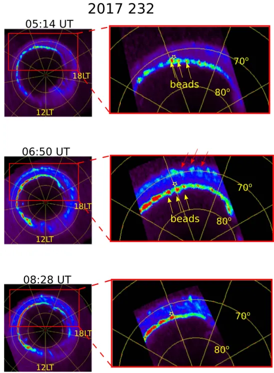
A few days before the end of its mission, the Cassini spacecraft approached very close to Saturn and captured unprecedented detailed views of its aurora. Here, we present Cassini Ultraviolet Imaging Spectrograph (UVIS; Esposito et al.2004) auroral observations taken on 2017 August 20 close to the end of the mission, together with simultaneous energetic electron observations obtained with the Cassini Low Energy Magnetospheric Measurement System (LEMMS) and Ion and Neutral Camera(INCA) measurements (Krimigis et al.2004). Figure1 shows a sequence of polar projections of Saturn’s southern aurora observed with the FUV channel of the UVIS instrument on 2017 August 20 DOY 232. During this sequence the spacecraft closely approached the planet. Its altitude changed from 7.2 to 5.3 RS and its subspacecraft latitude increased from 34°.9 to 40°.8 between the start of the first image and the end of the last one. For the construction of the projections we consider that the auroral emission peaks at 1100 km above the surface (Gérard et al. 2009). The projections display FUV emissions restricted to the 120–163 nm range in order to minimize contamination from solar reflection. The projected distance subtended by a pixel, changes proportionally with the range to the planet along the line of sight. More details on the method may be found in Grodent et al. (2011). In this study the images consist of three subimages and each subimage is taken over∼30 minutes. The starting time of each image is indicated on the top left of the panels of Figure1. The right side of the figure shows one of the three subimages (used to construct the complete image) which corresponds to the selected region indicated on the complete projection on the left side.
The polar projections displayed on the left side of Figure 1 illustrate the whole auroral region, while the right-hand side of the figure focuses on the nightside auroral region, where multiple detached and consecutive auroral spots are observed. One can easily discern 10–12 of them in the first image which are observed to enhance in the second image. Because of their shape, they are described hereafter as “auroral beads.” This term has been used at Earth to describe auroral features with similar morphological characteristics (Liang et al. 2008; Henderson2009; Rae et al.2009). The brightness of the beads ranges from 30 to 80 kR, while they move to higher latitudes. The longitudinal separation between beads is0.5 local hours. The auroral beads are spanning over a large local time sector (15h wide), from ∼20 LT to ∼11 LT via midnight at approximately 73° latitude. The rotating velocity is analyzed in detail in theAppendixof the paper. They can last for at least 3 hr, which is the whole duration sequence. The yellow stars show the magnetically mapped location of Cassini spacecraft at the time of the observation, indicating that Cassini’s location was close to the auroral beads. The mapping results were obtained using the internal field model of Dougherty et al. (2005) combined with the ring current model of Bunce et al. (2007). Given the location of Cassini close to the planet, the uncertainty in the mapping introduced by the magnetopause
distance inaccuracy is very limited, less than o.2° of latitude for a magnetopause distance change from 22 to 27RS. The auroral beads reported here have a much smaller scale than the features reported by Radioti et al.(2015), while it is unclear if the two structures correspond to similar drivers to those reported here. Auroral beads similar to those reported here are quite a common feature. They have been observed at various high-resolution data sets and mostly during the Grand Finale Cassini phase.
A similar pattern of repetitive spots is observed at lower latitudes, near∼70° along the “outer emission” of the auroral region, shown with the red arrows in the middle right panel of Figure1. The bead structures at lower latitudes are fainter(∼10 kR) than those observed at 70° and do not seem to be radially aligned with those at higher latitudes. The magnetospheric source region of the outer emission is located closer to the planet in the inner magnetosphere (e.g., Grodent et al.2010). The similarity of the auroral structures on the main and the outer emission, may suggest similar plasma processes (i.e., interchange instabilities), although the energy sources (e.g., pressure gradient force, shearflow, etc.) are likely different.
Simultaneously with the UV auroral observations, the INCA instrument on board Cassini observed enhancements of the ENA emissions, which are shown in Figure2. The images are 30 minute integrations centered at the indicated time, and the x-axis toward noon. In the past, similar ENA enhancements were associated with dynamical events and were closely correlated with UV transient features(Mitchell et al.2009; Radioti et al. 2013). In this study we use ENA observations in order to derive information about the spatial extent and the velocity of the heated plasma region related to the simultaneous UV emissions. The ENA enhancement covers a wide range of local times. At the beginning of the sequence the emission extends from ∼noon to midnight with a peak at 18LT and at the end of the sequence it reaches 06LT. It should be noted that part of the nightside emission between 7:20 UT and 9:16 UT is out of the field of view, because of the changes of Cassini trajectory (Cassini was at 11 RS and at 29° latitude at the beginning of the sequence, while at 7:12 UT it was located at 7 RSand at 37° latitude). The image taken at 7:12 UT shows that there is enhancement before and after 00 LT while a portion of the nightside region is missing, suggesting that there is continuous emission rotating from pre-midnight to post-mid-night, as documented numerous times in the literature (Krimigis et al. 2007; Carbary et al. 2008; Mitchell et al. 2009; Dialynas et al. 2013). During the time of the auroral observations from∼05:15 to 08:30 UT the ENA enhancement is located in the nightside region at the same local time sector as the spotty auroral emissions. As mentioned in the Introduction, the ENA emissions are indicative of a rotating heated plasma region moving between the orbits of Rhea(9 RS) and Titan(20.9 RS). It should be noted that this information is derived from equatorial projections of the ENA emission, which are not shown here. The heated plasma region is estimated to rotate with an angular velocity of∼70% of rigid corotation.
The LEMMS instrument on board Cassini, measured the differential intensities of energetic magnetospheric electrons simultaneously with UVIS. Figure 3 shows the differential intensities of energetic electrons from LEMMS channels C1 to C6, covering energies from 27 to 550 keV. The time interval covered by the UVIS observations is shown by the gray shaded
region on Figure 3. The electron intensities measured by the four lower channels C1, C2, C3, and C4 are observed to fluctuate and peak at approximately 05:00, 06:00, 07:00 and 08:00 UT, as indicated by the dashed lines. The green arrows show the intervals between two peaks, which are approxi-mately 1 hr. Contrary to the recurrent electron flux enhance-ments observed in Figure 3, the 1 hr quasi-periodic pulsations (sometimes referred to as QP60) described by Roussos et al. (2016) and Palmaerts et al. (2016) are mostly detected at higher energies(from channel C5 at 175 keV up to several MeV) but could be mixed with other electron populations at the lower energies considered in the present study. However, it is clear in
Figure3 that the enhancements discussed here are not present at energies above 175 keV. Additionally, they have a different morphology with a duration of about 10 minutes, except for the first peak, while each individual QP60 generally lasts for about 60 minutes with a rapidflux increase followed by a slow decay. We therefore consider that the events do not correspond to the same process that generates the QP60 reported by Roussos et al.(2016) and Palmaerts et al. (2016). We need to point out that the energetic electrons were measured at relatively high latitude (30°–40°), where only the relatively field-aligned population on the equator could arrive. We could roughly estimate the pitch angles for these electrons traveling to the
Figure 1.Sequence of polar projections of Saturn’s southern aurora obtained with the FUV channel of UVIS on board Cassini during the Cassini proximal orbits. The first image starts at 0514 UT and the last one at 0828 UT on DOY 232, 2017. Noon is to the bottom and dusk is to the right. The grid shows latitudes at intervals of 10° and meridians every 30°. Each panel of the right column displays one of the the subimages used to reconstruct the corresponding complete image on the left. The yellow arrows indicate some of the auroral beads on the main emission and the red ones those on the low latitude emission. The yellow star points out to the magnetically mapped location of the Cassini spacecraft at the time of the observation.
magnetic equator. Since Cassini’s footpoint is on the main emission, indicating that the magnetic field is traced to the outer magnetosphere(close to the open-closed field lines). The in situ measured magnetic field strength is about 50–200 nT (not shown in this Letter), and the equator magnetic strength in the outer magnetosphere is usually a few nT (<5 nT) (Yao et al. 2017a), so that the maximum equatorial pitch angle for the measured electrons is 18°. Usually this is almost at a
space-borne instrument’s angular resolution, and thus could be described as a goodfield-aligned population.
3. Auroral Beads at Saturn and Their Relation to Magnetospheric Instabilities
We suggest that the auroral beads observed in the midnight to dawn region (20LT to 11LT) reported here are related to plasma instabilities in the magnetosphere, which in turn
Figure 2.ENA emissions from Saturn’s magnetosphere starting on DOY 231 2017 at 23:57 and ending on 232 2017 at 09:16 UT. The images were integrated over 30 minutes and centered on the indicated time. The circles represent the orbits of Saturn’s innermost moons, namely Dione (∼6.2 RS) and Rhea (∼8.7 RS), together with
the orbit of Titan(∼20 RS). The z-axis is aligned with Saturn’s spin axis, the x-axis (highlighted in red) indicates the direction toward the Sun, and the y-axis points
to dusk.
Figure 3.Differential intensities of energetic electrons from channels C1 to C6 covering the energies from 27 to 550 keV of the Low Energy Magnetospheric Measurement System(LEMMS) instrument on board Cassini. The gray shaded region shows the interval during which UVIS captured the auroral emission shown in Figure1. The dashed lines mark the peaks of the electron intensities mainly seen in the low energy channels. The green arrows indicate the approximately hourly intervals between two peaks.
generate wave perturbations. At Earth, the auroral beads are often suggested to be driven by plasma ballooning instability, or balloon instability in mixture with shearflow named as shear flow-ballooning instability (i.e., Vinas & Madden 1986). It is intriguing that Saturn has auroral beads on its main aurora that are similar to those of Earth.
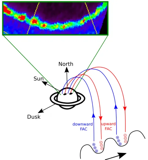
The ENA enhancements observed in this study(Figure2) are indicative of plasma pressure gradient forces, which create diamagnetic currents. The diamagnetic currents stretch the magneticfield. Pressure gradient in the stretched magnetic field is indeed a favorable condition for driving ballooning instabilities. Previous literature have revealed that flow shear exist on the dawn sector outer magnetopause between the solar wind plasma flow and rotating magnetospheric plasma (Masters et al. 2010; Delamere et al. 2013; Desroche et al. 2013). Therefore, shear flow and pressure gradient coexist in driving the main aurora. Regarding the similar morphology to the Earth auroral beads and the favorable conditions in driving plasma instability, we propose that the observed auroral beads at Saturn are driven by shear flow-ballooning instability, although we could not evaluate the relative importances between the shearflow and the plasma pressure gradient force. The quasi-periodic ∼1 hr fluctuations observed in the electron intensities measured by the three lower channels C1, C2, and C3 of LEMMS are consistent with drifting interchange structures in the inner plasma sheet similar to those reported by Motoba et al. (2015) and Yao et al. (2017c). These drifting structures can lead to an excess of electrons on one side of the wave structure crest and result in the creation offield-aligned currents (Roux et al. 1991). In that case, the electrons stream toward the ionosphere as upwardfield-aligned currents, which are carried by downward moving electrons and result in auroral intensifications such as the auroral beads observed here. The proposed mechanism is illustrated in Figure 4. Following the similar timing and perturbed nature of energetic electrons and auroral beads, we suggest that they are counterparts of the same process. As explained in the Appendix, it is difficult to know exactly how fast the beads structure rotated. We show the local time versus auroral intensity in Figure 5, and resolve all possible velocities, which are at angular velocities of 11%, 25%, 39% and 53%. The corresponding periods of electron pulsating are 189 minutes, 63 minutes, 38 minutes, and 27 minutes. The electrons are found to pulsate at∼1 hr, which is very consistent with the solution of 25%. Therefore, we suggest that the auroral beads structure rotated at an angular velocity of 25% rigid corotation, which corresponds to the ∼1 hr electron recurrence. As illustrated in Figure 5, the interchange plasma instability in the magnetosphere drives an interchange downward/upward field-aligned currents, and thus pulsating electron precipitations, causing auroral beads in the ionosphere.
The low latitude auroral emission(outer emission) shown in Figure 1 presents also auroral bead features that are morphologically similar to those reported on the main emission. We do not have enough evidence to argue about the origin of these low latitude auroral beads. Ballooning instability is not expected to be involved in the triggering process because of the low curvature drift in that region. They could be related to shear flow instabilities like the giant undulations in the terrestrial aurora which are explained in terms of shear flow instabilities in the inner magnetospheric
boundary driven by large shearflows between the inner plasma sheet and plasmasphere(Lui et al.1982).
Our study indicates that auroral bead structures are caused by fundamental plasma processes that commonly exist at Earth and Saturn and possibly at other planets in our solar system.
This work is based on observations with the UVIS instrument on board the NASA/ESA Cassini spacecraft. Z.Y. acknowledges the Strategic Priority Research Program of Chinese Academy of Sciences (grant No. XDA17010201). The research was supported by the Belgian Fund for Scientific Research(FNRS) and the PRODEX Program managed by the European Space Agency in collaboration with the Belgian Federal Science Policy Office. S.V.B. was supported by an STFC Ernest Rutherford Fellowship ST/M005534/1. Work at JHU/APL was supported by NASA under contracts NAS5-97271 and NNX07AJ69G and by subcontract at the Office of Space Research and Technology of the Academy of Athens. The German contribution of MIMI/LEMMS was financed in part by the Bundesministerium fur Bildung und Forschung (BMBF) through the Deutsches Zentrum fur Luft-und Raum-fahrt e.V. (DLR) and by the Max-Planck-Gesellschaft. The Cassini/UVIS, LEMMS and INCA data used in this study are available through the Planetary Data System (https://pds. nasa.gov).
Appendix
The Calculation of Auroral Bead Rotating Velocity It is challenging to trace each auroral bead between the two auroral images; therefore, we could not obtain an unambiguous calculation of the auroral bead structure’s rotating velocity. However, a generalized solution could be obtained, and the comparison with the other data set, i.e., electron recurrence, could help us to determine the most likely solution. Our methodology is described below step by step.
1. We integrate auroral intensity for the latitudes between 71° and 76°. As illustrated in Figure5, the integral area covers the bead structure well, so we obtain distributions of local time versus intensity for the beads’ auroral oval in the two images separated by 96 minutes.
2. It is clear that the bead structure has a wavelength of∼0.5 local hour, and there is a clear time shift between the two distributions, so that we can tell there was a propagation, although it is challenging to tell how many wavelengths are involved in the rotation.
3. If the rotation between the two beads structures is less than one wavelength(0-level connection as shown in the figure), the auroral structure shall have rotated ∼0.4 local hour in 96 minutes, corresponding to 11% rigid corota-tion velocity. If the rotacorota-tion between the two beads structures is more than one wavelength but less than two wavelengths (1-level connection), then the auroral structure shall have rotated0.9 local hour, corresponding to 25% of rigid corotation velocity. More generally, for n-level connection, the rotating velocity is(11 + 14*n)% of rigid corotation. Since the main auroral oval is known to rotate at 50%–60% of rigid corotation (Grodent et al. 2005; Yao et al. 2018), the poleward auroral structure, corresponding to a more distant magnetosphere, shall rotate at a lower angular velocity. Therefore we reason-ably suggest that n shall be not greater than 3. Note that
Figure 4.Schematic illustration of the build-up offield-aligned currents by magnetospheric plasma instabilities, which generate drifting interchange structures. These perturbations can lead to an excess of electrons on one side of the wave crest structure and result in the creation offield-aligned currents. Upward field-aligned currents carried by downward moving electrons result in localized auroral intensifications in the form of “beads.”
Figure 5.Top panel: the two auroral images shown in Figure1. Bottom panel: the distributions of local time vs. auroral intensity integrated between 71° and 76° in latitude for the two auroral images on the top panel. Thisfigure is to support the calculation of auroral beads structure’s rotating velocity. See the Annex for the detailed calculations.
the calculation does not involve the motion of space-craft’s footpoint, which would induce a small correction due to Doppler shift. The spacecraft’s footpoint moves along the planetary rotating direction (i.e., the same direction of auroral rotation) at an angular velocity of 0.1 local hour per hour, i.e., ∼4% of rigid corotation. Since the spacecraft’s footpoint and auroral beads rotate in the same direction, the relative speed of auroral beads in spacecraft’s frame is (7 + 14*n)% of planetary rigid corotation.
4. Since the wavelength is ∼0.5 local hour, the time difference between Cassini’s two successive auroral beads would be 13.2/(0.07 + 0.14*n) minutes, where n indicates the n-level connection. For n=(0, 1, 2, 3), the time difference between two auroral peaks would be (189 minutes, 63 minutes, 38 minutes, and 27 minutes). 5. The recurrent electron peaks have a time separation of
∼1 hr, which is consistent with the solution for n=1, i.e., 1-level connection. Therefore, we suggest the 1-level connection picture for the beads velocity, i.e., subcorota-tion with a velocity of 25% rigid corotasubcorota-tion.
ORCID iDs
Zhonghua Yao https://orcid.org/0000-0001-6826-2486 Denis Grodent https://orcid.org/0000-0002-9938-4707 B. Palmaerts https://orcid.org/0000-0003-2762-4334 E. Roussos https://orcid.org/0000-0002-5699-0678 K. Dialynas https://orcid.org/0000-0002-5231-7929 D. Mitchell https://orcid.org/0000-0003-1960-2119 J.-C. Gérard https://orcid.org/0000-0002-8565-8746 References
Badman, S. V., Jackman, C. M., Nichols, J. D., Clarke, J. T., & Gérard, J.-C. 2014,Icar,231, 137
Badman, S. V., Provan, G., Bunce, E. J., et al. 2016,Icar,263, 83
Bunce, E. J., Arridge, C. S., Clarke, J. T., et al. 2008,JGRA,113, 9209
Bunce, E. J., Cowley, S. W. H., Alexeev, I. I., et al. 2007,JGRA,112, 10202
Carbary, J. F., Mitchell, D. G., Brandt, P., Roelof, E. C., & Krimigis, S. M. 2008,JGRA,113, A05210
Clarke, J. T., Gérard, J.-C., Grodent, D., et al. 2005,Natur,433, 717
Delamere, P. A., Wilson, R. J., Eriksson, S., & Bagenal, F. 2013, JGRA,
118, 393
Desroche, M., Bagenal, F., Delamere, P. A., & Erkaev, N. 2013, JGRA,
118, 3087
Dialynas, K., Brandt, P. C., Krimigis, S. M., et al. 2013,JGRA,118, 3027
Dougherty, M. K., Achilleos, N., Andre, N., et al. 2005,Sci,307, 1266
Esposito, L. W., Barth, C. A., Colwell, J. E., et al. 2004,SSRv,115, 299
Gérard, J.-C., Bonfond, B., Gustin, J., et al. 2009,GeoRL,36, L02202
Grodent, D. 2015,SSRv,187, 23
Grodent, D., Gérard, J.-C., Cowley, S. W. H., Bunce, E. J., & Clarke, J. T. 2005,JGRA,110, 7215
Grodent, D., Gustin, J., Gérard, J.-C., et al. 2011,JGRA,116, 9225
Grodent, D., Radioti, A., Bonfond, B., & Gérard, J.-C. 2010,JGRA, 115, A08219
Henderson, M. G. 2009,AnGeo,27, 2129
Jinks, S. L., Bunce, E. J., Cowley, S. W. H., et al. 2014,JGRA,119, 8161
Kalmoni, N. M. E., Rae, I. J., Watt, C. E. J., et al. 2015,JGRA,120, 8503
Keiling, A. 2012,JGRA,117, A03228
Krimigis, S. M., Mitchell, D. G., Hamilton, D. C., et al. 2004,SSRv,114, 233
Krimigis, S. M., Sergis, N., Mitchell, D. G., Hamilton, D. C., & Krupp, N. 2007,Natur,450, 1050
Liang, J., Donovan, E. F., Liu, W. W., et al. 2008,GeoRL,35, L17S19
Lui, A. T. Y., Meng, C.-I., & Ismail, S. 1982,JGR,87, 2385
Masters, A., Achilleos, N., Kivelson, M. G., et al. 2010,JGRA,115, 7225
Meredith, C. J., Cowley, S. W. H., Hansen, K. C., Nichols, J. D., & Yeoman, T. K. 2013,JGRA,118, 2244
Mitchell, D. G., Krimigis, S. M., Paranicas, C., et al. 2009,P&SS,57, 1732
Motoba, T., Ohtani, S., Donovan, E. F., & Angelopoulos, V. 2015,JGRA,
120, 432
Nichols, J. D., Badman, S. V., Baines, K. H., et al. 2014,GeoRL,41, 3323
Palmaerts, B., Roussos, E., Krupp, N., et al. 2016,Icar,271, 1
Pu, Z. Y., Korth, A., Chen, Z. X., et al. 1997,JGR,102, 14397
Radioti, A., Grodent, D., Gérard, J.-C., et al. 2015,JGRA,120, 8633
Radioti, A., Grodent, D., GÈrard, J.-C., et al. 2017,JGRA,122, 6078
Radioti, A., Grodent, D., Jia, X., et al. 2016,Icar,263, 75
Radioti, A., Roussos, E., Grodent, D., et al. 2013,JGRA,118, 1922
Rae, I. J., Mann, I. R., Angelopoulos, V., et al. 2009,JGRA,114, A07220
Roussos, E., Krupp, N., Mitchell, D. G., et al. 2016,Icar,263, 101
Roux, A., Perraut, S., Robert, P., et al. 1991,JGRA,96, 17697
Talboys, D. L., Bunce, E. J., Cowley, S. W. H., et al. 2011,JGRA, 116, A04213
Vinas, A. F., & Madden, T. R. 1986,JGR,91, 1519
Yao, Z., Coates, A., Ray, L., et al. 2017a,ApJL,846, L25
Yao, Z., Pu, Z. Y., Rae, I. J., Radioti, A., & Kubyshkina, M. V. 2017c,GSL,
4, 8
Yao, Z., Radioti, A., Grodent, D., et al. 2018,JGRA,123, 8502