Assessing Deadwood Using Harmonized National Forest Inventory Data
Jacques Rondeux, Roberta Bertini, Annemarie Bastrup-Birk, Piermaria Corona, Nicolas Latte,
Ronald E. McRoberts, Go¨ran Ståhl, Susanne Winter, and Gherardo Chirici
Abstract: Deadwood plays an important role in forest ecological processes and is fundamental for the maintenance of biological diversity. Further, it is a forest carbon pool whose assessment must be reported for international agreements dealing with protection and forest management sustainability. Despite wide agreement on deadwood monitoring by national forest inventories (NFIs), much work is still necessary to clarify definitions so that estimates can be directly compared or aggregated for international reporting. There is an urgent need for an international consensus on definitions and agreement on harmonization methods. The study addresses two main objectives: to analyze the feasibility of harmonization procedures for deadwood estimates and to evaluate the impact of the harmonization process based on different definitions on final deadwood estimates. Results are reported for an experimental harmonization test using NFI deadwood data from 9,208 sample plots measured in nine European countries and the United States. Harmonization methods were investigated for volume by spatial position (lying or standing), decay classes, and woody species accompanied by accuracy assessments. Estimates of mean plot volume based on harmonized definitions with minimum length/height of 1 m and minimum diameter thresholds of 10, 12, and 20 cm were on average 3, 8, and 30% smaller, respectively, than estimates based on national definitions. Volume differences were less when estimated for various deadwood categories. An accuracy assessment demonstrated that, on average, the harmonization procedures did not substantially alter deadwood observations (root mean square error 23.17%). FOR. SCI. 58(3):269 –283.
Keywords: reference definitions, bridging functions, deadwood attributes, biodiversity indicator, carbon pool
D
EADWOOD IS ACKNOWLEDGED TO BE A CRITICAL ECOLOGICAL FACTORthat plays a fundamental role in forest ecosystems (e.g., Christensen et al. 2005, Lombardi et al. 2010). It is one of the most relevant com-ponents of forest biodiversity, and it represents an important forest carbon pool (Stokland et al. 2004, Woodall et al. 2009). Dead trees, stumps, and fine and coarse woody debris (CWD) are essential to forest ecosystem dynamics by providing food and habitat for taxa such as fungi, arthro-pods, birds, insects, and epiphytic lichens (Sippola and Renvall 1999, Bowman et al. 2000, Ferris et al. 2000, Siitonen et al. 2000, Simila¨ et al. 2003, Jonsson et al. 2005, Odor et al. 2006, Londsale et al. 2008, Winter and Mo¨ller 2008). Approximately 20 –25% of forest species depend ondecaying wood (Boddy 2001, Siitonen 2001), although de-cayed material is often viewed as a limited habitat resource for some organisms (Hagen and Grove 1999).
Deadwood is also considered to be an important indica-tor for assessing sustainable forest management and conser-vation of forest biodiversity (Ferris and Humphrey 1999, Hahn and Christensen 2004, Travaglini et al. 2007, Fischer et al. 2009). Deadwood was recognized as a biodiversity indicator for sustainable forest management by Forest Eu-rope, the former Ministerial Conference on the Protection of Forests in Europe (2003), and the Montre´al Process (Mon-tre´al Process 2005) and as one of 26 indicators selected for the Streamlining European 2010 Biodiversity Indicators ini-tiative to track temporal biodiversity changes in the context
Manuscript received May 25, 2010; accepted September 27, 2011; published online May 3, 2012; http://dx.doi.org/10.5849/forsci.10-057.
Jacques Rondeux, University of Lie`ge, Gembloux Agro-Bio Tech, Unit of Forest and Nature Management, Passage des De´porte´s 2, Gembloux, Namur 5030, Belgium—Phone: 00 32 81 62 22 28; [email protected]. Roberta Bertini, Universita` degli Studi di Firenze— [email protected]. Annemarie Bastrup-Birk, University of Copenhagen—[email protected]. Piermaria Corona, Universita` degli Studi della Tuscia—[email protected]. Nicolas Latte, University of Lie`ge, Gembloux Agro-Bio Tech, Unit of Forest and Nature Management—[email protected]. Ronald E. McRoberts, US Forest Service, Northern Research Station—[email protected]. Go¨ran Ståhl, Swedish University of Agricultural Sciences— [email protected]. Susanne Winter, Technische Universita¨t Mu¨nchen—[email protected]. Gherardo Chirici, Universita` degli Studi del Molise— [email protected].
Acknowledgments: This article is based on the activities carried out in WG3 of COST Action E43 “Harmonisation of National Forest Inventories: Techniques for Common Reporting.” We express our thanks to the chair of COST Action E43, Professor Erkki Tomppo, to the members of the steering committee (Klemens Schadauer, Emil Cienciala, Adrian Lanz, and Claude Vidal) and to those who were involved in the activities of WG3: Iciar Alberdi Asensio, Anna-Lena Axelsson, Anna Barbati, Nadia Barsoum, Jana Beranova, Urs-Beat Bra¨ndli, Vladimir Caboun, Catherine Cluzeau, Sebastiano Cullotta, Leandras Deltuva, Paulo Godinho-Ferreira, Nabila Hamza, Elmar Hauk, Albertas Kasperavicˇius, Marko Kovacˇ, Marco Marchetti, Helena Ma¨kela¨, Stefan Neagu, Jan-Erik Nilsen, Dieter Pelz, Tarmo Tolm, Tiina Tonteri, and Theocharis Zagas. For contributing deadwood data for the common DB, we gratefully acknowledge the following: Belgium: Jacques Rondeux and Nicolas Latte, Unit of Forest and Nature Management, University of Lie`ge (Gembloux Agro-Bio Tech); Switzerland: Urs-Beat Bra¨ndli and Ulrich Ulmer, Snow and Landscape Research (WSL), Swiss Federal Institute for Forest; Germany: Heino Polley, Johann Heinrich von Thu¨nen-Institut, Eberswalde; Denmark: Annemarie Bastrup-Birk and Thomas Nord-Larsen, Forest and Landscape, University of Copenhagen; Spain: Roberto Vallejo, Ministerio de Medio Ambiente y Medio Rural y Marino, and Iciar Alberdi Asensio and Sonia Conde´s, E.T.S.I. Montes de Madrid; Finland: Helena Ma¨kela¨, Finnish Forest Research Institute, Metla; Italy: Marco Marchetti, University of Molise; Sweden: Jonas Fridman and Anna-Lena Axelsson, Swedish University of Agricultural Sciences; United States of America: Forest Inventory and Analysis program of the Northern Research Station, US Forest Service. We acknowledge Alessandro Mastronardi (www.gm-studio.net) for the graphical three-dimensional rendering in Figure 2. We thank the associate editor of Forest Science and two anonymous reviewers who help us in improving the quality of an earlier draft of this article. This study was partially supported by the Italian Ministry of Research and University within the PRIN 2007 project “Innovative methods for the identification, characterization and management of old-growth forests in the Mediterranean environment.”
of the 2010 European target to halt the loss of biodiversity (European Environment Agency [EEA] 2007).
Deadwood is one of the five forest carbon pools defined by the Good Practice Guidance for Land Use, Land-Use Change and Forestry of the Intergovernmental Panel on Climate Change (Penman et al. 2003). For signatories to the United Nations Framework Convention on Climate Change, timely assessments of deadwood changes are essential for preparation of the required annual reports on greenhouse gas inventories (Cienciala et al. 2008, Woodall et al. 2008). The main source of information on the large-scale quan-tities and characteristics of deadwood are national forest inventories (NFIs) which, in recent decades, have incorpo-rated assessments of deadwood because of its relevance for biodiversity and for carbon pool monitoring (Puumalainen et al. 2003, Stokland et al. 2004, Bo¨hl and Bra¨ndli 2007). Because deadwood surveys have most often been developed for local conditions (Woldendorp et al. 2004, Travaglini et al. 2006), NFIs have adopted different definitions and in-ventorying methods. The result is that deadwood estimates are generally not comparable for different countries.
Estimation of reliable and comparable deadwood vol-umes at cross-country levels may be achieved using two possible approaches, standardization or harmonization. Ko¨hl et al. (2000) described standardization as a top-down approach that requires adoption of common international standards. The harmonization approach is, instead, a bot-tom-up approach based on the use of bridges to convert estimates based on national definitions to estimates based on international reference definitions (Ståhl et al. 2012).
This article presents the results of experimental investi-gations conducted by Working Group 3 (WG3) of COST Action E43 (Chirici et al. 2011), which dealt with harmo-nized assessments of forest biodiversity using NFI data. One component of these investigations focused on deadwood, in
particular, on developing and testing bridges for the harmo-nized assessment of multiple deadwood variables using NFI sample data voluntarily contributed by 10 countries: Bel-gium (BE), Switzerland (CH), Czech Republic (CZ), Ger-many (DE), Denmark (DK), Spain (ES), Finland (FI), Italy (IT), Sweden (SE) and the United States of America (USA). The harmonization tests are based on the assumption that the adopted reference definition for deadwood (Table 1, reference 1) is equivalent, except for the minimum diameter threshold, to the definitions adopted by individual NFIs. The impacts on deadwood estimates of different minimum diameter thresholds in the reference definitions are reported, and problems related to the implementation of the proposed harmonization bridges are discussed.
Because an international standard definition for dead-wood does not exist, adoption of reference definitions was indeed a critical step. For the purposes of this study, refer-ence definitions were defined on the basis of the discussions in COST E43 after a detailed analysis of national local definitions. More information related to the discussion and the general work program followed in COST E43 is detailed in Chirici et al. (2011). The reference definitions adopted are described in Table 1. In particular, deadwood volume at the plot level is defined as the sum of the volumes of standing and lying dead trees and coarse woody debris. The harmonization process we adopted is implemented at two different levels: for single deadwood elements and at ag-gregated plot level.
The process was repeated for three different deadwood reference definitions based on different minimum diameters (10, 12, and 20 cm). The results are presented using com-parisons of deadwood volume estimates based on the orig-inal NFI definitions and estimates resulting from the har-monization process, accompanied by an error estimation performed by assessing the quality of bridges.
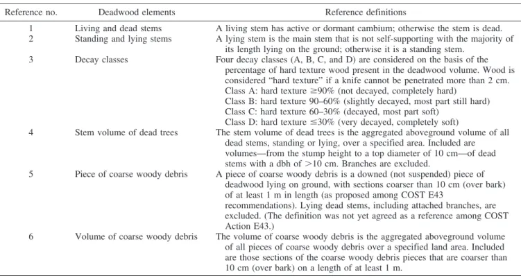
Table 1. Deadwood references adopted for the harmonization test.
Reference no. Deadwood elements Reference definitions
1 Living and dead stems A living stem has active or dormant cambium; otherwise the stem is dead. 2 Standing and lying stems A lying stem is the main stem that is not self-supporting with the majority of
its length lying on the ground; otherwise it is a standing stem. 3 Decay classes Four decay classes (A, B, C, and D) are considered on the basis of the
percentage of hard texture wood present in the deadwood volume. Wood is considered “hard texture” if a knife cannot be penetrated more than 2 cm. Class A: hard textureⱖ90% (not decayed, completely hard)
Class B: hard texture 90–60% (slightly decayed, most part still hard) Class C: hard texture 60–30% (decayed, most part soft)
Class D: hard textureⱕ30% (very decayed, completely soft)
4 Stem volume of dead trees The stem volume of dead trees is the aggregated aboveground volume of all dead stems, standing or lying, over a specified area. Included are volumes—from the stump height to a top diameter of 10 cm—of dead stems with a dbh of⬎10 cm. Branches are excluded.
5 Piece of coarse woody debris A piece of coarse woody debris is a downed (not suspended) piece of deadwood lying on ground, with sections coarser than 10 cm (over bark) of at least 1 m in length (as proposed among COST E43
recommendations). Lying dead stems, including attached branches, are excluded. (The definition was not yet agreed as a reference among COST Action E43.)
6 Volume of coarse woody debris The volume of coarse woody debris is the aggregated aboveground volume of all pieces of coarse woody debris over a specified land area. Included are those sections of the coarse woody debris pieces that are coarser than 10 cm (over bark) on a length of at least 1 m.
The final aim of this contribution is 2-fold: to demon-strate that the aggregation at the international level of dead-wood volume estimates acquired at the country level based on different definitions led to possible inaccuracies and to demonstrate that the harmonization of deadwood volume estimates on the basis of international common reference definitions is possible and feasible, even without the acqui-sition of new field data. The solutions we propose are limited by types of data we acquired within the framework of COST Action E43. We expect that our results will motivate future development of optimized harmonization techniques that can be operationally applied by the countries using their own NFI data.
For some countries, plot data were acquired within the framework of local forest inventories that are not formally national. For simplicity, we refer to all the data used in the test as from NFIs, even if they were sometimes acquired and provided by different authorities.
Materials
Methods and definitions adopted by the 10 countries involved in this study for assessing different deadwood components were acquired through questionnaires devel-oped by WG3 of COST Action E43 (Winter et al. 2008). The responses are summarized for the following deadwood features: sampling methods, spatial position (lying or stand-ing), decay classes, woody species, and volume calculation.
Sampling Methods
Deadwood elements are sampled in the field using plots or linear transects. When plots are used, all deadwood elements satisfying a specific definition and located within an area of predefined size, shape, and spatial location are measured. The transect approach (line intersect sampling [LIS]), which is adopted only for lying deadwood, consisted of measuring pieces that satisfy a specific definition and that intersected a sampling line of given length, origin, and direction (Warren and Olsen 1964, Van Wagner 1968, De Vries 1986).
Spatial Position
Eight countries adopted the lying and standing classes for classifying deadwood elements. Two countries used more complex systems of nomenclature with four or five classes to produce a more detailed description of the lying/standing condition of deadwood.
Decay Classes
Information on deadwood decomposition stage was available for nine countries. These countries used multiple decay classes ranging between 3 and 9 mainly based on deadwood color, texture, and softness.
Woody Species
Six countries determined the species of the deadwood; the others recorded only whether the element was from a coniferous or broadleaved tree. Some countries used a
spe-cific code such as “other” or “unidentified” for pieces for which the identification of the species was impossible be-cause of advanced decomposition.
Volume
National definitions and methods for calculating vol-umes of sampled deadwood elements were analyzed sepa-rately on the basis of two factors: sampling rules and vol-ume estimation procedures.
First, sampling rules are aimed to determine whether a deadwood element satisfies the adopted definition; if so, it is included in the sample, otherwise it is not considered for volume estimation. NFI field procedures are generally based on minimum diameter and length (or height) thresh-olds (Table 2) and are applied to elements inside a sampling unit (plot) or intersecting a line transect (LIS).
For standing deadwood, national minimum diameter thresholds varied between 4 and 20 cm, whereas minimum height was always the height at which diameter is measured. For eight countries, minimum height was 1.3 m aboveg-round, for Belgium minimum height was 1.5 m, and for the United States minimum height was 1.37 m (4.5 ft).
For lying deadwood, national thresholds included minimum diameter and minimum length. For lying stems, minimum diameter referred to the diameter measured at 1.3 m from the thicker end and varied from 7.5 to 12 cm; for lying deadwood pieces, minimum diameter referred to the diam-eter measured at the thinner end and varied from 6.4 to 20 cm. In the United States, which uses LIS, a minimum diameter of 7.6 cm is used for the point at which the line intersects the deadwood piece. Minimum lengths varied between 0.1 and 1.3 m.
Second, for volume estimation procedures, national def-initions vary with respect to the particular part of deadwood elements considered to estimate volume. Thus, even if two NFIs adopt the same sampling rules, the method used to estimate plot-level deadwood volume may differ, with the result that plot-level estimates may vary considerably.
The main differences among the 10 countries are re-ported in Tables 3 and 4.
The Common NFI Database
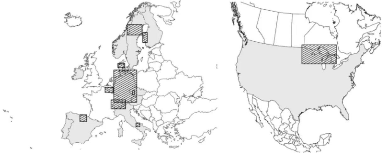
A common NFI database (DB) was populated with raw NFI deadwood data contributed from 4,842 plots from Eu-rope and 4,366 plots from the United States. Each country was responsible for the selection of plots for which data were contributed (Figure 1). The percentages of European plots by country are as follows: BE, 400 plots (8%); CH, 401 plots (8%); CZ, 302 plots (6%); DE, 790 plots (16%); DK, 1,458 plots (30%); ES, 775 plots (16%), FI, 336 plots (7%); IT, 192 plots (4%); and SE, 188 plots (4%).
The DB includes data for 9,208 plots, although dead-wood was observed and measured on only 4,985 plots. For the remaining plots, deadwood was not present or dead-wood elements did not satisfy local sampling rules. For all plots together, more than 23,000 deadwood pieces were observed and measured. All countries measured dbh and height for standing deadwood. However, consistency was
lacking for measurements of other deadwood attributes. One country did not record the height/length for standing snags (broken standing dead stem) and another country measured circumference at half the snag height. Measures for lying deadwood were for whole deadwood pieces for some countries but only for portions for other countries (Figure 2).
Methods
Overview
Bridges are methods for converting estimates based on national definitions to estimates based on reference defini-tions (Ståhl et al. 2012). Three types of bridges, depending on data availability relative to the reference definition and its thresholds, are used to make these conversions. When the scope of the data collected using national definitions is greater than the scope required by the reference definitions, a reductive bridge that discards some of the national data is used. When the scope of the data collected using national definitions is the same as that required by the reference definition, a neutral bridge is appropriate. Finally, when the scope of the data collected using the national definitions is less than that required by the reference definition, an ex-pansive bridge is necessary. Exex-pansive bridges are the most difficult to construct because a procedure for acquiring additional information is necessary.
For the deadwood harmonization investigations, bridges were applied at two levels: calculation of volume for indi-vidual deadwood pieces and per plot estimates by lying/ standing classes, decay classes, and woody species. In ad-dition, plot-level bridges were necessary because of different plot-level volume estimation procedures. Reduc-tive and neutral bridges were used at the level of individual deadwood pieces. Data were then aggregated at the plot level, and expansive bridges were applied when needed. The procedure was repeated for reference definitions corre-sponding to three minimum diameter thresholds: 10, 12, and 20 cm, labeled, respectively, Ref10, Ref12, and Ref20(Table 5).
To evaluate the accuracy of the harmonization process, deadwood volumes based on country definitions were com-pared with volumes predicted using bridges. The procedure was possible only for the subsample of plots for which the diameter threshold for the local deadwood definition com-pletely was less than that for the reference definition. Re-sults are reported for aggregations by spatial position.
Spatial Position
Neutral and reductive bridges were used to harmonize categories of spatial position into two categories: standing or lying. On the basis of the data available in the common DB, the bridge did not alter national definitions, because Table 2. Sampling rules used to identify deadwood pieces to be included in the field sample.
Country
Standing deadwood Lying deadwood
Type of deadwood Type of diameter Minimum diameter Minimum
height Type of deadwood
Type of diameter Minimum diameter Minimum length BE Standing trees dbh1 6.4 cm 1.5 m Lying trees and pieces
of deadwood
Thinner end 6.4 cm 1 m Broken snags At half height 6.4 cm 1.5 m
CH Standing trees and broken snags
dbh 12 cm not used Lying trees Thinner end 12 cm not used CZ Standing trees and
broken snags
dbh 5 cm 1.3 m Lying trees and pieces of deadwood
Thinner end 7 cm 0.1 m DE Standing trees and
broken snags
dbh 20 cm 1.3 m Lying trees and pieces of deadwood
Thinner end 20 cm 0.1 m DK Standing trees and
broken snags
dbh 4 cm 1.3 m Lying trees and pieces of deadwood
Thinner end 10 cm 1.3 m ES Standing trees and
broken snags
dbh 7.5 cm 1.3 m Lying trees Thinner end 7.5 cm 1.3 m
Lying pieces of deadwood
Thinner end 7.5 cm 0.3 m FI Standing trees dbh 10 cm 1.3 m Lying trees and pieces
of deadwood
Thinner end 10 cm 1.3 m Broken snags Top diameter2 10 cm 1.3 m
IT Standing trees and broken snags
dbh 4.5 cm 1.3 m Lying trees and pieces of deadwood
Thinner end 9.5 cm 0.1 m SE Standing trees and
broken snags
dbh 10 cm 1.3 m Lying trees Thinner end 10 cm 1.3 m
Lying pieces of deadwood
Thinner end 10 cm 1.3 m USA Standing trees and
broken snags
dbh3 12.7 1.3 m Lying trees and pieces
of deadwood Diameter at the line intersection point 7.6 cm 0.9 m
1dbh for BE is measured at a height of 1.5 m.
2dbh in the USA is measured at a height of 1.37 m (4.5 ft).
they were essentially equivalent to the reference definition (Table 1). For eight countries, the bridges were neutral, whereas for two countries they were reductive. Thus, dead trees and deadwood pieces recorded in the DB were as-signed to either a standing or lying spatial position.
Decay Classes
Neutral and reductive bridges were used to harmonize categories of decay classes by reassigning them from na-tional decay classes to reference classes (Table 1, reference 3). The bridges were neutral for four countries and reductive for six countries and were applied to all the dead trees and deadwood pieces.
Woody Species
Harmonization was conducted to assign all the dead-wood pieces to one of three classes: coniferous, broad-leaved, and not available.
Volume Calculation
Harmonization of deadwood estimates was conducted in two steps: intermediate harmonized volume estimates were calculated for each deadwood piece using NFI measure-ments in the DB for each of Ref10, Ref12, and Ref20and the
piecewise volume estimates from the first step were aggre-gated at the plot level and a second harmonization step was conducted using expansive bridges to obtain aggregated Table 3. National definitions for deadwood volume estimation.
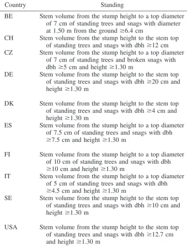
Country Standing Lying
BE Stem volume from the stump height to a top diameter of 7 cm of standing trees and snags with diameter at 1.50 m from the groundⱖ6.4 cm
Stem volume of the portion of lying trees and pieces of deadwood having a minimum diameterⱖ6.4 cm and a lengthⱖ1 m
CH Stem volume from the stump height to the stem top of standing trees and snags with dbhⱖ12 cm
Stem volume from the stump height to the stem top of lying trees with diameter at 1.30 m from the baseⱖ12 cm CZ Stem volume from the stump height to a top diameter
of 7 cm of standing trees and broken snags with dbhⱖ5 cm and height ⱖ1.30 m
Stem volume of the potion of lying trees and pieces of deadwood with diameterⱖ7 cm and length ⱖ0.1 m DE Stem volume from the stump height to the stem top
of standing trees and snags with dbhⱖ20 cm and heightⱖ1.30 m
Stem volume of lying trees and pieces of deadwood with a diameter at the thicker endⱖ20 cm and a length ⱖ0.1 m; volume of the stumps with diameter at felling height ⱖ60 cm and height ⱖ0.50 m
DK Stem volume from the stump height to the stem top of standing trees and snags with dbhⱖ4 cm and heightⱖ1.30 m
Stem volume of lying trees and pieces of deadwood with a diameter at thicker endⱖ10 cm and a length ⱖ1.3 m ES Stem volume from the stump height to a top diameter
of 7.5 cm of standing trees and snags with dbh ⱖ7.5 cm and height ⱖ1.30 m
Stem volume from the stump height to a top diameter of 7.5 cm of lying trees with dbhⱖ7.5 cm and length ⱖ1.30 m; volume of the portion of pieces of deadwood with diameterⱖ7.5 cm and length ⱖ0.30 m
FI Stem volume from the stump height to a top diameter of 10 cm of standing trees and snags with dbh ⱖ10 cm and height ⱖ1.30 m
Stem volume of the portion of lying trees and pieces of deadwood with a diameterⱖ10 cm and a length ⱖ1.3 m IT Stem volume from the stump height to a top diameter
of 5 cm of standing trees and snags with dbh ⱖ4.5 cm and height ⱖ1.30 m
Stem volume of the portion of lying trees and pieces of deadwood with a diameterⱖ9.5 cm and a length ⱖ0.1 m SE Stem volume from the stump height to the stem top
of standing trees and snags with dbhⱖ10 cm and heightⱖ1.30 m
Stem volume from the stump height to the stem top of lying trees with dbhⱖ10 cm and height ⱖ1.30 m; volume of whole pieces of deadwood with a diameter at thicker end ⱖ10 cm and a length ⱖ1.3 m
USA Stem volume from the stump height to the stem top of standing trees and snags with dbhⱖ12.7 cm and heightⱖ1.30 m
Volume of the portion of lying trees and pieces of
deadwood with a diameterⱖ7.6 cm and a length ⱖ0.9 m
Table 4. Methods for volume estimation for deadwood elements.
Volume function
Deadwood elements Standing
trees
Standing
snags Lying trees
Lying pieces of
deadwood Other Country volume tables (from stump height
to stem top, top diameter⫽ 0)
CH, DE, DK, SE, USA
CH, DE, DK, SE, USA
CH, SE Country volume tables, volume functions,
and taper curve models (from stump height to top diameter)
BE, CZ, ES, FI, IT
CZ, ES, FI ES
Smalian’s formula (Loetsch et al. 1973) FI ES, FI, SE, USA
Huber’s formula (Loetsch et al. 1973) BE BE, CZ, DE, DK BE, CZ, DE, DK DE (stump)
Frustum of cone IT
plot-level volume estimates because of differences in min-imum diameter and minmin-imum length thresholds between national and reference definitions.
Per Piece Harmonization
Bridges were developed to estimate volumes of individ-ual deadwood elements corresponding to the three reference definitions using data collected according to national defi-nitions. Reductive bridges were developed for use when the national thresholds were less than reference thresholds.
These bridges are in the form of reduction factors (Rf) with values between 0 and 1 and are applied to reduce the piecewise deadwood volumes provided by the countries. Values of Rf are calculated differently for different dead-wood components and are described in detail below.
Per Piece Harmonization of Standing Dead
Stems
According to the reference definitions (Table 1), stand-ing dead stem volume is the volume from the stump height Figure 1. Geographic location of the 9,208 plots used in the deadwood harmonization test.
Figure 2. Example of measures referred to the whole piece of lying deadwood (bottom) and referred to a part of it (top).
to a top over-bark diameter of 10 cm for stems with dbh of at least 10, 12, or 20 cm, depending on the reference definition used. When volume for individual standing dead stems is calculated, harmonization is necessary because of differences between national and reference definitions for both minimum dbh and minimum top diameter. When the national minimum dbh is smaller than the reference mini-mum dbh, a reductive bridge is used by selecting only standing dead stems in the DB whose dbhs are greater than the reference minimum dbh. When the national and refer-ence minimum dbhs are equal, the harmonization is through a neutral bridge used to convert values between different data formats. When the national minimum dbh is greater than the reference minimum dbh, an expansive bridge is necessary and is developed for application at the plot level. For Ref10, five reductive, two neutral, and three expansive
bridges were necessary, for Ref12, seven reductive, one
neutral, and two expansive bridges were necessary, and for Ref20, nine reductive bridges and one neutral bridge were
necessary.
The reference definition specifies a minimum top diam-eter of 10 cm (Table 1). Only one country adopted a national definition with a minimum top diameter threshold that was equal to that of the reference definition; in this case, as already made for the minimum dbh, a neutral bridge was used. For the other nine countries, reductive bridges in the form of reduction factors were used because their minimum top diameter thresholds were less than the reference thresh-old of 10 cm. Stem volume from stump height to top diameter d, Vtopd, can be defined as
Vtopd⫽ Rfdⴱ Vtop0. (1)
where Vtop0is total stem volume, Vtopdis stem volume to
top diameter d, and Rfdis the reduction factor.
Rfdin Equation 1 can be calculated from the estimation
system developed by Corona and Ferrara (1992) on the basis of the simple bole model proposed by Ormerod (1973):
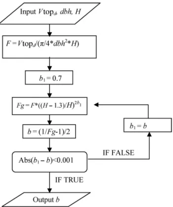
Rfd⫽ 1 ⫺ 关共H ⫺ 1.3兲/H兴2b⫹1⫻ 共d/dbh共2b⫹1兲/b兲. (2)
where Rfdis the reduction factor, H is the total height of the
stem, b is the exponent estimated for each tree, and d is the top diameter. The exponent b is estimated using an algo-rithm that modifies an initial estimate iteratively until the change between iterations is less than the prescribed amount (Figure 3). Stem volume to a reference top diameter, Vtopref,
is then defined as
Vtopref⫽ Rfref⫺dⴱ Vtopd. (3)
where ref is the minimum threshold for the reference defi-nition, Vtoprefis stem volume to the reference top diameter,
and Rfref–dis the reduction factor from Vtopdto Vtopref.
Stem volumes for different top diameters were first es-timated using Equation 1 with data available in the DB. Once Vtop10corresponding to the minimum top diameter of
10 cm for the reference definition was obtained using Equa-tion 1, Rfref–dwas calculated to convert stem volumes with
minimum top diameters of 5, 7, and 7.5 cm to stem volumes with minimum top diameters of 10 cm (Rf10 –5, Rf10 –7, and
Rf10 –7.5). The relationship between Rfref–d and dbh was
described using an equation of the form:
Rfref⫺d⫽ 1 ⫺ 共a ⴱ bdbh兲. (4)
The resulting equations (Figure 4) were then applied to individual standing dead stems in the DB to calculate the reference volume, Vtopref, using Equation 3 and data
col-lected according to national definitions (Table 3). The
Rfref–destimates obtained using Equation 4 were compared
to the available measured Rfref–dto assess the accuracy of
the models (Figure 5).
Per Piece Harmonization for Lying Deadwood
For purposes of calculating volume, the shape of a lying deadwood piece was assumed to be a frustum of a cone defined by maximum diameter (Dmax), minimum diameter
(Dmin), and length (L) as the linear distance between Dmax
and Dmin. The volume of such pieces (Figure 6), according
Table 5. Bridges used for deadwood harmonization at single-piece level (reductive and neutral bridges) and at plot level (expansive bridges).
Reductive bridges Neutral bridges
Expansive bridges Standing stems (whole trees and broken snags)
dbh (Ref10) BE, DK, IT, CZ, ES FI, SE CH, DE, USA
dbh (Ref12) BE, DK, IT, CZ, ES, FI, SE CH, DE, USA
dbh (Ref20) BE, DK, IT, CZ, ES, FI, SE,
CH, USA
DE
Height CH, CZ, FI, IT, SE,
USA, DK, ES, DE BE Lying stems (whole trees) (only for SE, ES, and CH)
Diameter at 1.30 m (Ref10) ES SE CH
Diameter at 1.30 m (Ref12) ES, SE CH
Diameter at 1.30 m (Ref20) ES, SE, CH
Length CH, ES, SE
CWD (no data for Switzerland) and lying stems
Diameter (Ref10) BE, CZ, ES, USA, IT DK, SE DE, FI
Diameter (Ref12) BE, CZ, ES, USA, IT, DK, SE, FI DE
Diameter (Ref20) BE, CZ, ES, USA, IT, DK, SE, FI DE
to the adopted reference definitions, is the volume of the portions of a piece of lying deadwood with a minimum diameterⱖ10 cm (or 12 or 20 cm) and having at least 1-m length (VCWDref). Volumes for lying deadwood components
with diameters less than the reference definition threshold and equal to or greater than the reference threshold were calculated using the following procedure. Two cases had to be analyzed, depending on the availability of end diameters of the pieces of wood considered.
If the countries provide Dminand Dmax, they are used to
calculate a tapering rate R expressed as follows:
R⫽Dmax⫺ Dmin
L . (5)
The rate is used to estimate the lengths of components with diameters less than the reference diameter and the lengths of components with diameters greater than or equal to the reference diameter. From those lengths and the two diam-eters, volumes are estimated using the Smalian formula (Loetsch et al. 1973, Rondeux 1999b). The reduction factor
r is then calculated as the ratio of two volumes: the volume
of the component with diameter greater than or equal to the reference diameter and the total volume:
r⫽ VDminⱖ10 VDminⱖ10⫹ VDmin⬍10
. (6)
The volume of the piece of wood corresponding to the reference definition is the product of the reduction factor r (Equation 6) and the volume of the piece provided by the NFI.
If the countries do not provide Dminand Dmax because
only the diameter in the middle of every piece of wood is measured (Dmid), R cannot be calculated. Therefore,⌬D ⫽
Dmax ⫺ Dmin must be estimated using data from other
countries that measure both Dmaxand Dmin. Several
possi-bilities exist to solve this problem, for example, using Dmid
as an explanatory variable of R. We preferred a linear regression model of the form,⌬D ⫽ a ⫹ b ⫻ L (Figure 7), constructed to estimate ⌬D for every piece of wood of a given length L. For coniferous species, the model and its coefficient estimates are ⌬D ⫽ 0.0202 ⫹ 0.0018L, where ⌬D and L are expressed in m, with r2⫽ 0.5272 and root
mean square error (RMSE)⫽ 54%. For broadleaved spe-cies, the model and its coefficient estimates are ⌬D ⫽ 0.0367⫺ 0.0122 L, with r2⫽ 0.5107 and RMSE ⫽ 47%. These linear models were then applied to pieces for which Dmax and Dmin were not provided as a means of
Figure 3. The algorithm for the calculation of the exponent b of equation 2. For the meaning of Vtop0, dbh, and H we refer
to equations 1 and 2. [Abs (b1ⴚ b) means “absolute value” of
the difference (b1ⴚ b)]. Adapted from Corona and Ferrara
(1992).
Figure 4. Example of the function from equation 4 used for local minimum top diameters of 5 cm (Rf10 –5).
Figure 5. Example of the regression found for reduction factor Rf5–10) and its estimation made throughout the
estimating R (Equation 5). Therefore, Dmaxand Dmincan be
estimated as follows:
Dmax⫽ Dmid⫹ R ⴱ L/2.
Dmin⫽ Dmid⫺ R ⴱ L/2.
The same steps presented in the case of countries where
Dmaxand Dminwere measured were then used.
Per plot harmonization
Per plot harmonization was needed for countries whose minimum diameter, minimum height, or minimum length used in the selection of the deadwood elements to be mea-sured in the field were greater than the reference definition thresholds (Table 4). In these cases, expansive bridges are needed to estimate the portion of deadwood volume not measured in the field using national definitions.
Per plot harmonization was necessary for six countries for Ref10, five for Ref12, and three countries for Ref20
(Table 5). For countries not requiring expansive bridges, the harmonized estimate of deadwood volume per plot is the
sum of the harmonized volumes of all the deadwood pieces expressed on a per ha basis.
Per plot harmonization was accomplished by construct-ing plot-level models of the relationship between the na-tional deadwood volumes (VNFI) and the volumes estimated
using the reference definitions (Vref). Using NFI data for a
sample of plots from Czech Republic, Italy, and Spain, the relationship between VNFIand Vrefwas modeled as
Vref⫽ f 共VNFI兲. (7)
Data for these three countries were used because their national deadwood thresholds were less than the reference thresholds. Linear models of the form
Vref⫽ a ⴱ VNFI⫹ b, (8)
were constructed for different deadwood components ac-cording to local definitions. A total of 16 models were used (Table 6).
Accuracy Assessment
An accuracy assessment was conducted to analyze the similarity between observed deadwood volumes and vol-umes estimated by bridges. A formal assessment requires deadwood volume data based on both local and reference definitions for the same field plots. Because such data were not available in the common DB, we used a simulation procedure. First, all deadwood elements were selected from the common DB for each country whose minimum diameter thresholds for their national definitions were less than the corresponding minimum diameter thresholds for the refer-ence definitions. Selections were made for standing and lying components separately and for each reference (Ref10,
Ref12, and Ref20); in aggregate for both standing and lying
deadwood and for all three references, elements were avail-able for 1,359 plots. Second, for this reduced data set, deadwood volume, Vref*, was calculated for each plot
with-out application of bridges. For example, for a country whose national definition included a minimum diameter threshold ofⱕ10 cm, Vref*⫽ V10*was calculated using only elements
from the country whose diameters were at least 10 cm. Third, for the same reduced dataset, an NFI minimum diameter threshold of 12 cm was simulated by deleting from Figure 6. Schematic diagram of the division of a lying piece of deadwood in two components on the basis
of the reference definition with a minimum diameter of 10 cm. The right part has a minimum diameter <10 cm; its volume is VDmin>10. The left part has a minimum diameter >10 cm; its volume is VDmin>10. The
proportion of VDmin>10when the left side part has a length >1 m is used to calculate the reference volume VCWD10.
Figure 7. Example of the linear regression found for the category “Conifers” (⌬D ⴝ Dmaxⴚ Dmin).
the dataset all elements whose diameters were⬍12 cm. An expansive bridge in the form of equation 8 was then used to calculate Vref ⫽ V10. This procedure was implemented for
Vref* ⫽ V10*with NFI diameters of 12 and 20 cm and for
Vref* ⫽ V12* with NFI diameter of 20 cm. For lying and
standing components separately, comparisons of Vref* and
Vref included analyses of distributions of their differences,
simple linear regressions of Vref*against Vref(Figure 8) and
calculation of RMSE as RMSE⫽
冑
1 n冘
i⫽1 n 共Vrefⴱi⫺ Vrefi兲 2where i denotes specific deadwood elements.
Results
Deadwood volume per ha was estimated for each plot for which data were recorded in the DB using four definitions: the original deadwood volume estimated by the countries using their national definitions (VNFI) and harmonized
esti-mates, VRef10, VRef12, and VRef20, corresponding to the three
reference definitions with minimum diameter thresholds of 10, 12, and 20 cm. Per plot deadwood volume was also estimated for the reference categories of spatial position (lying or standing), decay classes (four classes), and woody species (three classes). For each European plot, the forest category based on the European system of nomenclature implemented by the EEA (2007) was also available, whereas for American plots three forest types based on the main three species composition classes were used. These
estimates are based only on data in the DB contributed by 10 countries, and do not necessarily represent a probability sample for the countries. Therefore, the estimates are not construed to be representative of actual large area condi-tions in any of the 10 countries.
The accuracy results are reported first, because they provide the foundation for many of the other results. Accu-racy assessments were conducted separately for the three references and for the lying and standing spatial compo-nents. For the lying component, data could be used for 1,208 Figure 8. Result of the accuracy assessment: relationship between Vrefand Vref*(in m
3
haⴚ1) for the 1,359 plots consid-ered. The trend line corresponds to Yⴝ X.
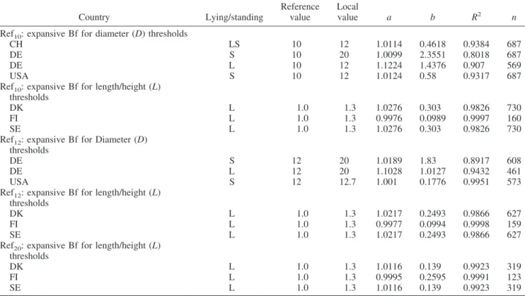
Table 6. Characteristics of the parameters for expansive per plot bridges.
Country Lying/standing
Reference value
Local
value a b R2 n
Ref10: expansive Bf for diameter (D) thresholds
CH LS 10 12 1.0114 0.4618 0.9384 687
DE S 10 20 1.0099 2.3551 0.8018 687
DE L 10 12 1.1224 1.4376 0.907 569
USA S 10 12 1.0124 0.58 0.9317 687
Ref10: expansive Bf for length/height (L)
thresholds
DK L 1.0 1.3 1.0276 0.303 0.9826 730
FI L 1.0 1.3 0.9976 0.0989 0.9997 160
SE L 1.0 1.3 1.0276 0.303 0.9826 730
Ref12: expansive Bf for Diameter (D)
thresholds
DE S 12 20 1.0189 1.83 0.8917 608
DE L 12 20 1.1028 1.0127 0.9432 461
USA S 12 12.7 1.001 0.1776 0.9951 573
Ref12: expansive Bf for length/height (L)
thresholds
DK L 1.0 1.3 1.0217 0.2493 0.9866 627
FI L 1.0 1.3 0.9977 0.0994 0.9998 159
SE L 1.0 1.3 1.0217 0.2493 0.9866 627
Ref20: expansive Bf for length/height (L)
thresholds
DK L 1.0 1.3 1.0116 0.139 0.9923 319
FI L 1.0 1.3 0.9995 0.2595 0.9991 123
SE L 1.0 1.3 1.0116 0.139 0.9923 319
The following information is reported: the country for which the bridge was developed, the deadwood component for which the function was developed (lying or standing), the local threshold used, the parameters a and b of the equation, the accuracy of the models in terms of R2and the number of plots
plots. A simple linear regression of plot-level volumes ob-tained from field observations versus volume predictions obtained from bridges produced estimates of the intercept-slope pair as (0.84, 0.95), which are close to the ideal values of (0, 1) and R2 ⫽ 0.95. In addition, more than 82% of deviations between observations and predictions, expressed as proportions of observations, were ⬍0.50. In addition, RMSE as a proportion of the observation mean was approx-imately 0.47. For the standing component, data could be used for 151 plots. Estimates of the intercept-slope pair were (0.18, 0.96), R2⫽ 0.97; more than 85% of deviations expressed as a proportion of observations were⬍0.25, and RMSE as a proportion of the observation mean was approx-imately 0.26.
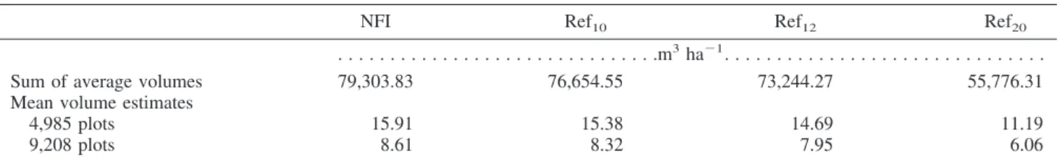
The effects of harmonization are illustrated by compar-ing estimates based on the national definitions and the three reference definitions (Table 7). For plots represented in the DB, in terms of the sum of the per ha average deadwood volume estimates, the differences between the original NFI values (VNFI) and the three adopted reference definitions
(VRef10, VRef12, and VRef20) ranged between 3 and 30%. Of the
4,985 DB plots with VNFI⬎ 0, the mean harmonized
dead-wood volume estimates decrease as the minimum diameter threshold increases: mean per plot deadwood volume de-creases from VNFI ⫽ 15.91 m
3
ha⫺1to VRef20⫽ 11.19 m
3
ha⫺1. On the total of 9,208 plots, including the 4,223 plots for which deadwood volume is 0, independently of the definitions adopted, VRef10, VRef12, and VRef20decreased from
8.61 m3 ha⫺1 of VNFI to 8.32, 7.95, and 6.06 m 3
ha⫺1, respectively (Table 7).
Because the reference definitions relate only to minimum diameter thresholds, their use does not alter the distribution of deadwood volume estimates by categories of spatial position, decay class, or woody species (Table 8). The ratio of estimates of lying deadwood volumes to estimates of standing deadwood volumes and, similarly, the percentages of deadwood volumes by species classes (conifer-broadleaved-unclassified) are quite stable over the different definitions.
The distributions of deadwood volume estimates by the
four harmonized decay classes (Table 1, Reference 3) were also quite stable relative to the definitions. Percentages of estimates of deadwood volume by the five classes (A, B, C, D, and not available) range from 16 to 8%.
For all 14 European forest categories (Barbati et al. 2006), deadwood volume estimates decreased when chang-ing from the NFI definitions to the three reference defini-tions (Table 9; Figure 9). The percentage reducdefini-tions in deadwood volume estimates when changing from VNFI to
VRef10, VRef12, and VRef20, respectively, were smallest for
alpine coniferous forests and greatest for broadleaved ever-green forests.For the three American forest types, changing
from VNFIto VRef10produced an increase in mean deadwood
volume estimates of 3.2% for aspen forest, 3.8% for paper birch, and 4.5% for balsam poplar and changing from VNFI
to VRef12had a minimal effect (⫺1.6, ⫺0.1, and ⫺0.4%).
The effects on mean deadwood volume estimates when changing from VNFI to VRef10 vary by country and range
from a 3.3% increase to a 30.3% decrease. Changing from
VNFI to VRef12produced decreases in mean deadwood
esti-mates by country ranging from 1.1 to 40.5% and changing from VNFIto VRef20produced decreases ranging from 9.8 to
63.5%.
Discussion
Although the majority of NFIs collects data to facilitate nationwide forest monitoring, deadwood is a relatively new variable for most NFIs (Rondeux 1999a, Rondeux and San-chez 2010). In most cases the methodologies adopted for its assessment have not been specifically studied or tested, so it is difficult to determine whether any particular approach is better than another. However, the increasing emphasis on multifunctional forest uses, and sustainable forest manage-ment has led to expansion of the scopes of NFIs, particularly in areas related to biodiversity and carbon pools. Thus, the emergence of methodological problems related to selection of variables, data collection and processing protocols, and cross-country harmonization of estimates should not be surprising. The study herein reported is the first attempt to Table 7. Effects on harmonization based on estimates of the sum of average deadwood volumes per ha and mean harmonized deadwood volumes per ha using plots with VNFI>0 (4,985 plots) and total available plots (9,208 plots).
NFI Ref10 Ref12 Ref20
. . . .m3ha⫺1. . . .
Sum of average volumes 79,303.83 76,654.55 73,244.27 55,776.31
Mean volume estimates
4,985 plots 15.91 15.38 14.69 11.19
9,208 plots 8.61 8.32 7.95 6.06
NFI for values based on original national definitions; Ref10, Ref12and Ref20, for values after harmonization based on reference definitions.
Table 8. Comparison between deadwood volume estimates based on original national definitions (VNFI) and the three reference
definitions tested (VRef12, VRef12, and VRef20).
NFI Ref10 Ref12 Ref20
Spatial components: standing/lying 71/29 73/27 73/27 74/26
Species: coniferous/broadleaved/unclassified 55/40/5 57/39/4 57/40/3 56/41/3 Decay classes (A/B/C/D/not available)1 16/21/44/11/8 15/21/46/10/8 15/21/46/10/8 15/21/46/10/8
Values are expressed as a percentage considering standing/lying components, species, and decay classes.
harmonize deadwood volume estimates using NFI data, the primary source of information for national and international reporting purposes. The investigations were based on a sample of NFI data from 4,842 plots from nine European countries and 4,366 plots from the United States.
Harmonization efforts focused on constructing bridges to produce estimates based on reference definitions using data collected according to national definitions. The effects on
overall estimates and estimates by categories of spatial position, decay class, and species composition using three different minimum diameters thresholds (10, 12, and 20 cm) were evaluated. Harmonization of categories of spatial po-sition, decay class, and woody species was relatively easy because national and reference definitions were nearly equivalent. Thus, most bridges were either reductive or neutral. For reductive and neutral bridges, plot estimates Figure 9. Mean volumes (in m3
haⴚ1) per European forest categories and American forest types before (NFI) and after harmonization (Ref10, Ref12, and Ref20). Data represent the mean of 9,208 plots. Descriptions of European forest categories (1–14) and American forest types (901, 902, and 904) are in Table 9.
Table 9. Results of the harmonization test carried out on 9,208 plots.
Identification Name NFI Ref10 Ref12 Ref20 Plots
Europe
1 Boreal forest 4.25 2.83 2.77 2.21 365
2 Hemiboreal and nemoral Scots pine forest 8.3 7.24 6.84 5.73 359
3 Alpine coniferous forest 20.88 20.29 19.88 18.8 311
4 Atlantic and nemoral oakwoods, Atlantic ashwoods, and dune forest
8.86 7.19 6.7 4.11 101
5 Oak-hornbeam forest 7.17 6.66 6.37 5.12 549
6 Beech forest 11.39 11.11 10.82 9.41 435
7 Mountainous beech forest 9.33 8.8 8.6 7.55 274
8 Thermophilous deciduous forest 2.97 2.49 2.35 1.58 366
9 Broadleaved evergreen forest 0.16 0.08 0.07 0.03 133
10 Coniferous forests of the Mediterranean, Anatolian and Macronesian regions
2.95 2.7 2.64 2.09 121
11 Swamp forest 4.23 3.85 3.78 3.44 146
12 Floodplain forest 9.53 6.77 6.36 5.21 31
13 Non-riverine alder, birch, or aspen forest plantations 4.37 3.62 3.52 3.43 82
14 Plantations and self-sown exotic forest 5.75 4.52 4.12 2.81 1,569
USA
901 Aspen forest 9.34 9.64 9.19 6.55 3,465
902 Paper birch forest 14.58 15.13 14.6 10.73 636
904 Balsam poplar forest 9.57 10 9.61 7.42 265
Average deadwood volume (in m3ha⫺1) by European forest categories (EEA, 2006) and American forest types before the harmonization (column NFI)
were assumed not to be influenced by plot shape or size and not by sampling procedures for selecting deadwood ele-ments. Harmonization to accommodate differences in piece-and plot-level estimation protocols were more difficult piece-and in some cases required expansive bridges.
Inevitably, the application of bridges, especially expan-sive bridges, alters the original values acquired in the field; thus, quantification of effects of the bridges is important. A formal accuracy assessment is possible only on the basis of data acquired in the field for this purpose; however, such data were not available for this study. Therefore, a proce-dure was used for a subsample of the dataset: 1,208 plots for lying deadwood components and 151 plots for standing deadwood components. In general, deviations between plot-level observations and plot-plot-level predictions obtained using the bridges were comparable and small. However, there was a slight tendency for the bridges to overestimate volume for plots with small observed volumes and to underestimate volumes for plots with large observed volumes. In addition, deviations tended to increase when the minimum diameter threshold increased, probably because of the combination of two effects: the average volume of deadwood elements also increases with increasing minimum diameter and a large minimum diameter required a greater alteration of the orig-inal data during the harmonization process. Deviations for the harmonization of lying deadwood were greater than those for standing deadwood. Because the average volumes for the two element types were similar, the differences in deviations were probably due to the fact that for standing deadwood, harmonization tended to entail only minor alter-ations of observed volumes.
On the basis of lessons learned from this experiment carried out in COST Action E43, multiple recommendations may be proposed for facilitating harmonization of dead-wood variable estimates. First, information on the geo-graphic location of deadwood pieces should be collected in the field. Such information would facilitate harmonization with respect to plot size and configuration. Second, classi-fication of deadwood elements on the basis of their lying or standing spatial position in a manner that permits easy conversion to reference classes would be useful. Third, classification of lying deadwood and dead stems with re-spect to piecewise volume calculation methods (e.g., Huber and Smalian) would contribute to greater ease in harmoni-zation. Fourth, acquisition of minimum and maximum di-ameters and the length between them for all CWD elements, regardless of the national approaches to volume calculation, would greatly contribute to development of taper models and development of bridges. Fifth, acquisition of data for a top minimum diameter of 0 in addition to the data for the national minimum top height would permit estimation that would be harmonized with respect to any reference threshold.
This study does not address all aspects of the harmoni-zation of deadwood estimates, so considerable work still remains. Stump volume was not included in estimates be-cause sufficient data were not available. Differences in overall deadwood volume and volume by decay class for different silvicultural techniques, stand types, age classes, dominant species composition classes, and forest structure
classes were not been studied because relevant information was not available (Gore and Patterson 1986). Nevertheless, further studies in these areas are necessary because, for example, intensely managed forests probably contain less deadwood than accumulates naturally because dead trees are generally removed (Siitonen et al. 2000, Hill et al. 2005, Lombardi et al. 2010). Finally, the relationships between deadwood and threats to biodiversity that may result from predicted climatic changes should also be investigated (Thomas et al. 2004).
Conclusions
Five primary conclusions may be drawn from this study. First, and most importantly, the results clearly indicate that bridges that produce harmonized deadwood estimates based on reference definitions may be constructed, regardless of the national definitions used to collect the data. Further, the accuracy of the harmonization process we used is estimated to be 23.17%. Second, harmonization of categories of spa-tial position, decay class, and woody species class was relatively easy, although harmonization with respect to piece- and plot-level estimation was more difficult because expansive bridges were more frequently required. Third, as should be expected, harmonized estimates based on refer-ence definitions may deviate considerably from estimates based on national definitions. However, rather large ranges of minimum diameter thresholds (10 –20 cm) had little effect on the proportions of deadwood volume estimates by spatial position, decay class, woody species, and forest category. In addition, consistency in this regard for Euro-pean and American deadwood data separately suggests the possibility of global harmonization. Fourth, as noted in the Discussion, considerable harmonization work yet remains. Fifth, the recommendations of WG3 of COST Action E43 provided in the Discussion should be given serious consid-eration, regardless of whether individual countries are in-clined to modify features of their NFIs.
Literature Cited
BARBATI, A., P. CORONA, ANDM. MARCHETTI. 2006. European
forest types. Categories and types for sustainable forest man-agement reporting and policy. EEA Tech. Rep. No. 9.
Euro-pean Environmental Agency, Copenhagen, Denmark. BODDY, L. 2001. Fungal community ecology and wood
decompo-sition processes in angiosperms: From standing tree to com-plete decay of coarse woody debris. Ecol. Bull. 49:43–56. B ¨OHL, J.,ANDU.B. BRANDLI¨ . 2007. Deadwood volume assessment
in the third Swiss National Forest Inventory: Methods and first results. Eur. J. For. Res. 126(3):449 – 457.
BOWMAN, J.C., D. SLEEP, G.J. FORBES,ANDM. EDWARDS. 2000. The association of small mammals with coarse woody debris at log and stand scale. For. Ecol. Manag. 129(1–3):119 –124. CHIRICI, G., S. WINTER, AND R.E. MCROBERTS. 2011. National
Forest Inventories: Contributions to forest biodiversity assess-ments. Springer, New York.
CIENCIALA, E., E. TOMPPO, A. SNORRASON, M. BROADMEADOW, A. COLIN, K. DUNGER, Z. EXNEROVA, B. LASSERRE, H. PE
-TERSSON, T. PRIWITZER, G. SANCHEZ, AND G. STÅHL. 2008. Preparing emission reporting from forests: Use of National Forest Inventories in European countries. Silva Fenn. 42(1): 73– 88.
CHRISTENSEN, M., K. HAHN, E. MOUNTFORD, P. O´DOR, D. ROZEN
-BERGER, J. DIACI, T. STANDOVAR, S. WIJDEVEN, S. WINTER, T. VRSKA,ANDP. MEYER. 2005. Dead wood in European beech (Fagus sylvatica) forest reserves. For. Ecol. Manag. 210: 267–282.
CORONA, P.,ANDA. FERRARA. 1992. Un metodo semplificato per la trasformazione delle tavole a doppia entrata per la cubatura di fusti interi in tavole assortimentali. Ital. For. Mont. 3:144 –157.
DE VRIES, P.G. 1986. Sampling theory for forest inventory: A
teach-yourself course. Springer Verlag, Berlin. 399 p.
EUROPEANENVIRONMENTAGENCY. 2007. Halting the loss of
bio-diversity by 2010: Proposal for a first set of indicators to monitor progress in Europe. EEA Tech. Rep. No. 11. European
Environment Agency, Copenhagen, Denmark.
FERRIS, R., AND J.W. HUMPHREY. 1999. A review of potential biodiversity indicators for application in British forests.
For-estry 72(4):313–328.
FERRIS, R., A.J. PEACE, ANDA.C. NEWTON. 2000. Macrofungal communities of lowland Scots pine (Pinus sylvestris L.) and Norway spruce (Picea abies (L.) Karsten) plantations in Eng-land: Relationships with site factors and stand structure. For.
Ecol. Manag. 131(1/3):255–267.
FISCHER, R., O. GRANKE, G. CHIRICI, P. MEYER, W. SEIDLING, S. STOFER, P. CORONA, M. MARCHETTI, AND D. TRAVAGLINI. 2009. Background, main results and conclusions from a test phase for biodiversity assessments on intensive forest monitor-ing plots in Europe. iForest 2(1):67–74.
GORE, J.A.,ANDW.A. PATTERSON. 1986. Mass of downed wood
in northern hardwood forests in New Hampshire: Potential effects of forest management. Can. J. For. Res. 16(2):335–339. HAGEN, J.M.,AND S.L. GROVE. 1999. Coarse woody debris. J.
For. 97:6 –11.
HAHN, K., ANDM. CHRISTENSEN. 2004. Deadwood in European forest reserves—A reference for forest management. P. 181–191 in Monitoring and indicators for forest biodiversity in
Europe—From ideas to operationality, Marchetti, M. (ed.).
Issue 51. European Forest Institute, Joennsu, Finland. HILL, D., M. FASHAM, G. TUCKER, M. SHEWRY,AND P. SHAW.
2005. Handbook of biodiversity methods—Survey, evaluation
and monitoring. Cambridge Univ. Press, Cambridge, UK.
573 p.
JONSSON, B.G., N. KRUYS, AND T. RANIUS. 2005. Ecology of species living on dead wood—Lessons for dead wood manage-ment. Silva Fenn. 39:289 –309.
K ¨OHL, M., B. TRAUB,ANDR. P ¨AIVINEN. 2000. Harmonization and standardization in multi-national environmental statistics–Mis-sion impossible? Environ. Monit. Assess. 63(2):361–380. LOETSCH, F., F. Z ¨OHRER,ANDK.E. HALLER. 1973. Forest
inven-tory, vol. II, p. 356 –365. BLV Verlagsgesellschaft, Mu¨nchen.
LOMBARDI, F., G. CHIRICI, M. MARCHETTI, R. TOGNETTI, B. LASSERRE, P. CORONA, A. BARBATI, B. FERRARI, S. DIPAOLO, D. GIULIARELLI, F. MASON, F. IOVINO, A. NICOLACI, L. BIAN
-CHI, A. MALTONI, AND D. TRAVAGLINI. 2010. Deadwood in forest stands close to old-growthness under Mediterranean conditions in the Italian Peninsula. It. J. For. Mount. Environ. 65(5):481–504.
LONDSALE, D., M. PAUTASSO, AND O. HOLDENRIEDER. 2008. Wood-decaying fungi in the forest: Conservation needs and management options. Eur. J. For. Res. 127:1–22.
MINISTERIAL CONFERENCE ON THE PROTECTION OF FORESTS IN
EUROPE. 2003. Improved Pan-European indicators for
sustain-able forest management as adopted by the MCPFE expert level meeting 7– 8 October 2002, Vienna, Austria. Available online
at www.mcpfe.org; last accessed Oct. 1, 2008.
MONTREAL´ PROCESS. 2005. The Montre´al Process. Available on-line at www.rinya.maff.go.jp/mpci/; last accessed Apr. 1, 2008. ODOR, P., J. HEILMANN-CLAUSEN, M. CHRISTENSEN, E. AUDE, K.W.VANDORT, A. PILTAVER, I. SILLER, M.T. VEERKAMP, R. WALLEYN, T. STANDOVAR, A.F.M VAN HEES, J. KOSEC, N. MATOSEC, H. KRAIGHER,ANDT. GREBENC. 2006. Diversity of dead wood inhabiting fungi and bryophytes in semi-natural beech forests in Europe. Biol. Conserv. 131:58 –71.
ORMEROD, D.W. 1973. A simple bole model. For. Chron. 49:136 –138.
PENMAN, J., M. GYTARSKY, T. HIRAISHI, T. KRUG, D. KRUGER, R. PIPATTI, L. BUENDIA, K. MIWA, T. NGARA, K. TANABE, F. WAGNER(EDS.). 2003. Good Practice Guidance for Land Use,
Land-Use Change and Forestry. Institute for Global Environ-mental Strategies for the IntergovernEnviron-mental Panel on Climate Change, Ipcc National Greenhouse Gas Inventories Programme.
Available online at www.ipcc-nggip.iges.or.jp/public/gpglulucf/ gpglulucf.htm; last accessed Nov. 1, 2008.
PUUMALAINEN, J., P. KENNEDY,ANDS. FOLVING. 2003. Monitor-ing forest biodiversity: A European perspective with reference to temperate and boreal forest zone. J. Environ. Manag. 67(1):5–14.
RONDEUX, J. 1999a. Forest inventories and biodiversity. Unasylva 196:35– 41.
RONDEUX, J. 1999b. La mesure des arbres et des peuplements
forestiers. Les Presses agronomiques de Gembloux, Gembloux,
Belgium, 522 p.
RONDEUX, J.,ANDC. SANCHEZ. 2010. Review of indicators and field methods for monitoring biodiversity within national forest inventories. Core variable: Deadwood. Environ. Monit. Assess. 164(1– 4):617– 630.
SIITONEN, J. 2001. Forest management, coarse woody debris and saproxylic organisms: Fennoscandian boreal forests as an ex-ample. Ecol. Bull. 49:11– 41.
SIITONEN, J., P. MARTIKAINEN, P. PUNTTILA,ANDJ. RAUH. 2000. Coarse woody debris and stand characteristics in mature man-aged and old-growth boreal mesic forests in southern Finland.
For. Ecol. Manag. 128(3):211–225.
SIMILA¨, M., J. KOUKI, AND P. MARTIKAINEN. 2003. Saproxylic beetles in managed and seminatural Scots pine forests: Quality of deadwood matters. For. Ecol. Manag. 174(1):365–381. SIPPOLA, A., ANDP. RENVALL. 1999. Wood decomposing fungi
and seed-tree cutting: A 40 year perspective. For. Ecol. Manag. 115(2–3):183–201.
STÅHL, G., E. CIENCIALA, G. CHIRICI, A. LANZ, C. VIDAL, S. WINTER, R.E. MCROBERTS, J. RONDEUX, K. SCHADAUER,AND
E. TOMPPO. 2012. Bridging national and reference definitions for harmonizing forest statistics. For. Sci. 56:214 –223. STOKLAND, J.N., S.M. TOMTER,ANDU. S ¨ODERBERG. 2004.
Devel-opment of deadwood indicators for biodiversity monitoring: Experiences from Scandinavia. P. 207–226 in Monitoring and
indicators of forest biodiversity in Europe—From ideas to operationality. EFI Proc. No. 51. European Forest Institute,
Joennsu, Finland.
THOMAS, C.D., A. CAMERON, R.E. GREEN, M. BAKENESS, L.J. BEAUMONT, Y.C. COLLINGHAM, B.F.N. ERASMUS, M. FER
-REIRA DESIEQUEIRA, A. GRAINGER, L. HANNAH, L. HUGHES, B.
HUNTLEY, A.S. VAN JAARSVELD, G.F. MIDGLEY, L. MILLES, M.A. ORTEGA-HUERTA, A.T. PETERSON, O.L. PHILLIPS, AND
S.E. WILLIAMS. 2004. Extinction risk from climate change.
Nature 427:145–148.
TRAVAGLINI, D., A. BARBATI, G. CHIRICI, F. LOMBARDI, M. MAR
-CHETTI, ANDP. CORONA. 2007. ForestBIOTA data on dead-wood monitoring in Europe. Plant Biosyst. 141(2):222–230.
TRAVAGLINI, D., F. MASON, M. LOPRESTI, F. LOMBARDI, M. MAR
-CHETTI, G. CHIRICI,ANDP. CORONA. 2006. Deadwood survey-ing experiments in alpine and Mediterranean forest ecosystems.
Ann. Ist. Sper. Selv. 30:71– 86.
VANWAGNER, C.E. 1968. The line intersect method in forest fuel sampling. For. Sci. 14:20 –26.
WARREN, W.G.,ANDP.F. OLSEN. 1964. A line intersect technique for assessing logging waste. For. Sci. 13:267–276.
WINTER, S., G. CHIRICI, R.E. MCROBERTS, E. HAUK, AND E. TOMPPO. 2008. Possibilities for harmonizing national forest inventory data for use in forest biodiversity assessments.
For-estry 81(1):33– 44.
WINTER, S., AND G. M ¨OLLER. 2008. Microhabitats in lowland beech forests as monitoring tool for nature conservation. For.
Ecol. Manag. 255:1251–1261.
WOODALL, C.W., L.S. HEATH, ANDJ.E. SMITH. 2008. National inventories of down and deadwoody material forest carbon stocks in the United States: Challenges and opportunities. For.
Ecol. Manag. 256(3):221–228.
WOODALL, C.W., H. VERKERK, J. RONDEUX,ANDG. STÅHL. 2009. Who’s counting dead wood? EFI News 2/2009:12–13. WOLDENDORP, G., R.J. KEENAIN, S. BARRY,ANDR.D. SPENCER.
2004. Analysis of sampling methods for coarse woody debris.