Statistical classification methodology of SHOALS
3000 backscatter to mapping coastal benthic habitats
Antoine Collin, Antoine Cottin, Bernard Long
Department of Geology INRS-ETE, University of Québec
Québec, Canada
Pim Kuus, John Hughes Clarke
Department of University of New Brunswick
Fredericton, Canada
Phillippe Archambault
Institut des Sciences de la mer Université du Québec à Rimouski
Rimouski, Canada
Gunho Sohn, John Miller
Department of Applied Engineering York University
Toronto, Canada
Abstract— The Scanning Hydrographic Operational Airborne
LiDAR Survey (SHOALS) consists of a bathymetric LiDAR system which provides high precision measurements of water depth. Even though the acquisition is focused on depth accuracy, the return signal, i.e. waveform, contains other relevant information because of integration signatures from the water surface, the water column and the sea-bed. This paper highlights the benthic characterization in extracting statistical parameters derived from the bottom backscatter. In applying multivariate analysis (K-means), it is significantly proven that signals derived from habitat, described as statistically homogeneous throughout ground-truth analysis, are (1) similar within an intra-habitat view, while they are (2) different between themselves.
Keywords-components: bathymetric LiDAR; waveform; multivariate analysis; habitat classification
I. INTRODUCTION
Airborne laser (or LiDAR) bathymetry (ALB) is a technique for measuring the depths of relatively shallow, coastal waters from the air using a scanning, pulsed laser beam [1-3]. Indeed, it is a well suited technique to the shore mapping because its laser system enables to provide accurate Digital Depth Model (DDM) in a 1-50 m vertical range with a 25 cm height precision. The depth detection essentially depends on water turbidity. Compared to passive remote-sensing systems, this active state-of-the-art technology can measure the depth at two to three times the Secchi depth [4]. Moreover, topographic surveys above the water surface can be conducted simultaneously, in order to draw seamless Digital Terrain Model (DTM), key-component of a better comprehension of the littoral structures and dynamics.
Some researchers have begun to use the peak bottom signal parameter from the SHOALS waveform data. They used the intensity to map the marine environment by draping intensity images over DDM, or by combining intensity with passive image data using more sophisticated sensor or data fusion algorithms [5-9].
Despite the presence of noise (optical sensors) and the integration of several parameters acting within the water surface, water column and bottom return, typical benthic waveform patterns are also evident, suggesting that laser temporal signal may indeed comprise important, ad hoc and added information related to the characterization of the shore habitat. The main objective of this paper is to investigate relationships between the bottom return waveform and related sediment and benthic-community patterns in four sites located near shore in Paspébiac, Gulf of St Lawrence, Canada (Fig. 1).
II. SHOALSSYSTEM
In hydrographic mode, the SHOALS emits the 532 nm and 1064 nm wavelengths from a Nd-YAG laser with a beam divergence of 0.45 mrad. The first radiation (blue-green) is typically used for the sea-bed detection because of its high water penetration, while the second wavelength (near infrared) allows measuring the water surface because of its high water absorption. The transmitted laser pulses are partially reflected from the water surface and from the sea bottom back to the airborne receiver. In effect, distances to the sea surface and bottom can be calculated by measuring the times of flight of the pulses to those locations and knowing the speed of light in air and water. The SHOALS bathymetric scanning reaches 3 kHz with a fixed nadir angle of 20°. In this paper the only density mode 4 m x 4 m was used.
III. METHODOLOGY
LiDAR intensity is the ratio of received energy to transmitted energy. Its physical meaning is linked with parameter measurements integrated during the beam path. The bathymetric SHOALS return may be divided into three main parts: the water surface, the water column, and the benthic (bottom) return [4]. As the nadir angle, the altitude and all the loss parameters were correctly sustained during the survey, the signal equation is:
Figure 1. Rasterization of maximum elevation derived from SHOALS return over Paspébiac (15.77 km2, 1 m resolution)
PR = W PT R * e (-2KD)
(1) PR : Received power of bathymetric LiDAR signal W: Constant combining loss factors PT : Transmitted power R: Benthic Reflectance
K: Diffusive attenuation coefficient of water D: Benthic depth
Furthermore, transforming (1) with natural log, we can obtain an equation that is linear in depth (2):
Ln PR = Ln (W PT R) – 2KD (2) Equation (2) stands for the framework of the normalization stage.
A. Study site
LiDAR data for this analysis were collected by SHOALS on July 2nd, 2006 over the subtidal nearshore of Paspébiac, southern Gulf of St. Lawrence, Quebec, Canada. Paspébiac is hydro- dynamically characterized by high energy. Two sand pits, nourished by quaternary deposits and the east swell, join themselves to draw a typical triangle. The study area was covered by a series of 16 eastwest overlapping flight lines at 270 ± 5 m altitude enabling a swath width of 196 ± 3.6 m and a sample spacing of 4 m. LiDAR intensity was recorded in function of time. Only the blue-green deep channel (out to 4 channels) was analyzed in this paper. The signal is delimited by 250 electroVolt and 160 nanoseconds (Fig. 2).
For this experiment, only four subsets of the SHOALS data were chosen for exploratory data analysis. These four areas (100 m x 10 m) were specified by the information derived from ground truth. Seafloor photographs were extracted with a digital high-resolution (5 megapixels) camcorder fitted with a wide-angle lens and placed in a waterproof case. Two 250 W light sources allowed (1) adjustment of the illumination according to the water turbidity, (2) the position of the camcorder to the bottom, or (3) both factors. The system was mounted on a tetrapod frame that included a reference ruler to evaluate the size of material of the seabed. Throughout this study area, for each of these four stations surveyed, ten 0.16 m2 images of the seafloor were collected when the camcorder reached the bottom.
Figure 2. Segmentation of a typical raw bathymetric LiDAR backscatter. This one was acquired at 3.37 depth.
B. Normalization
Since SHOALS data were acquired at different depths, to compare echoes with one another, a depth normalization procedure was applied to correct both the strength of the recorded intensity values and the temporal spreading of the backscatters [10-11]. Note that since the laser beam is a cone, the size of the sampled area, or footprint, is physically linked to the acquisition depth.
C. Data analysis
In order to determine the relevant utility of the bathymetric laser data to discern differences in benthic characteristics, deviations in the composition of habitats, visualized with ground truth, were emphasized. This was processed in two steps. First, to quantify the surface covered by the sediment and the epi-macrobenthos, a grid of 100 uniformly distributed points was superimposed on the photographs, and what was under each point was identified to give an estimate of the percentages of the surface covered by each component [12]. Second, the aerial percentages were submitted to multivariate statistical analyses to classify the stations by their similarity. The matrix of 40 stations by 17 variables, corresponding to the species- and sediment-type aerial percentages, was used to compute similarity matrices on selected variables using the Bray-Curtis index [13]. The similarity matrices were then submitted to average linkage hierarchical clustering to classify the stations [14]. For each resulting classification, the mean relative aerial density and percentage of contribution to within groups similarity were computed for the main components of the group [13].
After the depth-normalization, the signal processing consists of extracting the portion of the waveform which contains the relevant benthic information. The ad hoc portion is called “benthic return” (Fig. 2). The signal curvature is studied by the first derivative. As a result it becomes possible to retrieve the depth-normalized benthic signal. Then two approaches were used to extract variables from backscatters. The first approach computed a series of descriptive statistical variables (Ev) derived from normalized raw signals, and the second treatment dealt with the same statistical variables but derived from Gaussian-fitted curves. Both methods yield a data table of 11
extracted variables (columns) and 164 backscatters (rows). Following an unsupervised classification, both data matrices were submitted to one type of multivariate statistical analysis. Indeed, a K-means clustering analysis was performed on the correlation matrices of the Ev variables.
IV. RESULTS A. Ground-truth sampling
The hierarchical clustering applied to the similarity matrix computed from the combination of sediments and epi-macrobenthos aerial percentages identified four groups (Table 1) from the photographs analysis. The four groups are actually mainly sorted by both their sediment and biological composition: group 1 (G1) can be related to Laminaria sp. on bedrock habitat, group 2 (G2) to fine sand habitat, group 3 (G3) to Echinoidea on fine sand habitat and group 4 (G4) to Laminaria sp. and Zostera sp. on fine sand habitat.
B. SHOALS classifications
The results of the SHOALS classifications of both extraction methods are given in Table II. The resulting classifications showed a close correspondence between the laser pattern and the benthic habitat. Taking account into the discrimination of the four previous habitats, the number of clusters was determined for K = 4. For both methods, the optimal split level was reached at the third split and each of clusters stand for an inherent habitat. Moreover, Overall accuracies resulting from both batches were 100 %.
Complementary to statistical reports (Table II), biplots of both clusterings (Fig. 3 and Fig. 4) bring information about scattering patterns of the return signals projected onto the two first principal components. Statistically, point clouds (Fig. 4) attributed to the three habitats comprising sand did not display any difference of the dispersion (G2-G3: Z = 1.18; G2-G4: Z = 1.46; G3-G4: Z = 1.52; p = 0.001), while the algae on bedrock habitat showed a point cloud significantly more scattered (G1-G2: Z = 8.34; G1-G3: Z = 9.02; G1-G4: Z= 4.35; p = 001).
TABLE I. THE RELATIVE AERIAL DENSITY AND CONTRIBUTION TO WITHIN-GROUP SIMILARITY FOR THE MACROBENTHOS AND SEDIMENTS AERIAL
PERCENTAGES IN EACH GROUP IDENTIFIED WITH HIERARCHICAL CLUSTERING.
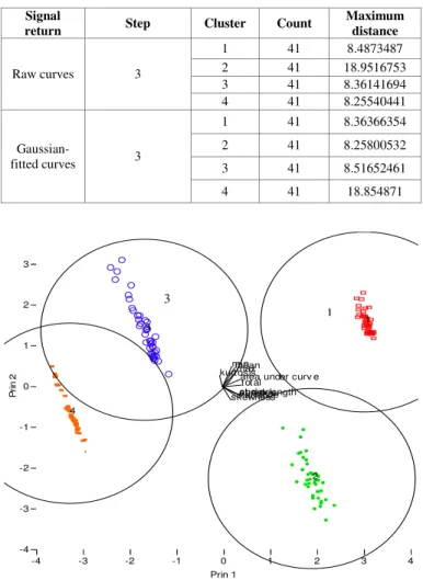
TABLE II. THE K-MEANS CLUSTERING SHOALS CLASSIFICATION SHOWING CLUSTER CHARACTERISTICS FOR BOTH EXTRACTION METHODS.
Signal
return Step Cluster Count
Maximum distance 1 41 8.4873487 2 41 18.9516753 3 41 8.36141694 Raw curves 3 4 41 8.25540441 1 41 8.36366354 2 41 8.25800532 3 41 8.51652461 Gaussian-fitted curves 3 4 41 18.854871 -4 -3 -2 -1 0 1 2 3 P ri n 2 1 2 3 4 mean t ot al max min v ariance st dev abs dev skewness kurt osis curv e length area under curv e
-4 -3 -2 -1 0 1 2 3 4
Prin 1
Figure 3. Clustering with a K-means approach applied to statistical parameters derived from normalized benthic backscatters [●: Laminaria sp. on
bedrock (G1); □: Fine sand (G2); ■: Echinoidea on fine sand (G3); ○:
Laminaria sp. and Zostera sp. on fine sand (G4)]
-3 -2 -1 0 1 2 P ri n 2 1 2 3 4 mean total max min v ariance st dev abs dev skewness kurtosiscurv e length
area under curv e
-4 -3 -2 -1 0 1 2 3 4
Prin 1
Figure 4. Clustering with a K-means approach applied to statistical parameters derived from Gaussian curves fitted with normalized benthic
backscatters [●: Laminaria sp. on bedrock (G1); □: Fine sand (G2); ■: Echinoidea on fine sand (G3); ○: Laminaria sp. and Zostera sp. on fine sand
(G4)]
Groups Features Relative aerial density (%)
Contribution to similarity (%) Laminaria sp. 66.3 38.4 Asteroidea 1.9 30.5 1 Pebbles>80 mm 19.8 29.7 2 Sand 98.6 97.2 Echinoidea 26.6 51.3 Laminaria sp. 7.2 2.3 3 Sand 57.1 42.7 Laminaria sp. 63.9 57.4 Zostera marina 9.4 17.9 4 Sand 10.3 21.3 1 3 1 1-4244-1212-9/07/$25.00 ©2007 IEEE. 3180
DISCUSSION
First, the ground-truth analysis of photographs showed that (1) the intra-site and (2) the inter-site variabilities of the sediment and benthic-community types were, respectively, sufficiently low and high to be statistically discriminated. Second, bathymetric LiDAR backscatters can significantly differentiate between the four characterized habitats.
As the species encountered in our study live in preferred sediment types, we assumed that the sediment distribution was implicitly involved in the SHOALS discrimination of the benthic communities, but was generally not controlling the observed patterns. Some ancillary factors are also used to characterize a habitat such as water depth, seafloor geomorphology, habitat complexity, current speed, food supply, temperature range, predation pressure, and disturbance by fishing activities [15]. These environmental factors certainly influence the pattern of benthic-community distribution and should be taken into account in the interpretation of SHOALS classifications.
Depth variation has been shown in the literature to affect our capacity to detect and differentiate remote sensed signatures [16-17]. Even with depth normalization that accounts for temporal spreading and power, it is not possible to compensate for the effect of surveying a large versus a small habitat area. Both classifications reached perfect accuracies, probably due to this depth-dependency. To assess the impact of such variation, depth-dependent data tables should be extracted and analyzed. Without a proper depth normalization procedure, the effects of uncorrected depth fluctuations are likely to overshadow the variation inherent in the nature of the seabed and fatally link the laser signatures to depth-related variables. To perform an accurate depth normalization, since the rate at which the light is absorbed as it travels through water was estimated instead of being precisely measured, corrective measures of the attenuation coefficient of water should be taken.
In identifying a larger variability about the distance point-seed on the Laminaria sp. on bedrock (G1) than the three sand habitats, this scattering can reveal biophysical aspects of the habitat sounded. Thus, the greater heterogeneity bound to algae on bedrock site can highlight the growth of entropy, while sand habitats, characterized by denser point clouds, show bio-sediment sites more homogeneous, in this study. Within this outlook, it will be relevant to find out specific sets of extracted variables that could be used to correctly and significantly identify the nature of the habitat surveyed, based on SHOALS signatures.
ACKNOWLEDGMENT
A. Collin gratefully acknowledges support from the Geoide project, the Institut National de la Recherche Scientifique – Eau Terre et Environnement (INRS-ETE) and Fisheries and Oceans Canada.
REFERENCES
[1] Hickman G.D. and J.E. Hogg, 1969, “Application of an airborne pulsed laser for near-shore bathymetric measurements”, Remote Sens. of Env., 1, Elsevier, New York, 47-58.
[2] Guenther G.C., 1985, “Airborne laser hydrography: System design and performance factors”, NOAA Professional Paper Series, National Ocean Service 1, National Oceanic and Atmospheric Administration, Rockville, MD, 385 pp.
[3] Guenther G.C., 1989, “Airborne laser hydrography to chart shallow coastal waters”, Sea Technology, March, Vol. 30, No. 3, 55-59.G.C. [4] Guenther G.C., A.G. Cunningham, P.E. LaRocque and D.J. Reid,
“Meeting the Accuracy Challenge in Airborne LiDAR Bathymetry” presented at EARSel, Dresden, 2000.
[5] Park J.Y., R.L. Shrestha, W.E. Carter and G.H. Tuell, 2001, “Land-cover Classification Using Combined ALSM (LIDAR) and Color Digital Photography,” presented at ASPRS Conference, St. Louis, Missouri, April 23-27, 2001.
[6] Tuell G. H., “ Data Fusion of Airborne Laser Data with Passive Spectral Data”, 3RD Annual Airborne Hydrography Workshop, Corte Madiera, CA, July 2002.
[7] Park J.Y., 2002, Data Fusion Techniques for Object Space Classification Using Airborne Laser Data and Airborne Digital Photographs, Ph.D. Dissertation, Department of Civil and Coastal Engineering, Univeristy of Florida, Gainesville, Florida.
[8] Carter W., R. Shrestha, G. Tuell, D. Bloomquist and M. Sartori, 2001, “Airborne Laser Swath Mapping Shines New Light on Earth’s Topography” Eos, Transactions, American Geophisical Union, Vol. 82, No. 46, November 13, 2001, Pp 549, 550, 555.
[9] Wang C. and W. Philpot, 2001, “Assessment of Airborne Lidar Data for Detection of Shallow Ocean Bottom Change”, 3RD Annual Airborne Hydrography Workshop, Corte Madiera, CA, July 2002.
[10] Clarke P. A., and L. J. Hamilton, 1999, “The ABCS Program for the analysis of echo sounder returns for acoustic bottom classification”, DSTO-GD-0215”, Defence Science and Technology Organisation, Aeronautical and Maritime Research Laboratory, Melbourne, Victoria, Australia.
[11] Hamilton L. J., 2001, “Acoustic seabed classification systems.”, DSTO-TN-0401, Defense Science and Technology Organisation, Aeronautical and Maritime Research Laboratory, Fishermans Bend, Victoria, Australia.
[12] Archambault P., K. Banwell and A. J. Underwood, 2001, “Temporal variation in the structure of intertidal assemblages following the removal of sewage”, Marine Ecology Progress Series, 222: 51-62.
[13] Clarke K. R. and R. M. Warwick, 1994, “Change in marine communities: an approach to statistical analysis and interpretation”, Natural Environment Research Council, UK. 144 pp.
[14] Legendre P. and L. Legendre, 1998, Numerical Ecology, 2nd English edn. Elsevier, Amsterdam. 853 pp.
[15] Kostylev V. E., B. J. Todd, G.B.J. Fader, R.C. Courtney, G.D.M. Cameron and R. A. Pickrill, 2001, “Benthic habitat mapping on the Scotian Shelf based on multibeam bathymetry, surficial geology and seafloor photographs”, Marine Ecology Progress Series, 219: 121-137. [16] Hewitt J. E., S. F. Thrush, P. Legendre, G. A. Funnell, J. Ellis, and M.
Morrison, 2004, “Mapping of marine soft-sediment communities: integrated sampling for ecological interpretation”, Ecological Applications, 14:1203–1216.
[17] Hutin E., Y. Simard and P. Archambault, 2005, “Acoustic detection of a scallop bed from a single-beam echosounder in the St. Lawrence” ICES
Journal, 62:966-983.