HAL Id: hal-00776320
https://hal.archives-ouvertes.fr/hal-00776320
Submitted on 15 Jan 2013
HAL is a multi-disciplinary open access
archive for the deposit and dissemination of
sci-entific research documents, whether they are
pub-lished or not. The documents may come from
teaching and research institutions in France or
abroad, or from public or private research centers.
L’archive ouverte pluridisciplinaire HAL, est
destinée au dépôt et à la diffusion de documents
scientifiques de niveau recherche, publiés ou non,
émanant des établissements d’enseignement et de
recherche français ou étrangers, des laboratoires
publics ou privés.
Antenna Radiation in Typical Office Environment:
Theoretical Modeling and Measurements
Zaher Sayegh, Mohamed Latrach, Fumie Costen, Wafa Abdouni, Ghaïs El
Zein, Gheorghe Zaharia
To cite this version:
Zaher Sayegh, Mohamed Latrach, Fumie Costen, Wafa Abdouni, Ghaïs El Zein, et al.. Antenna
Radiation in Typical Office Environment: Theoretical Modeling and Measurements. European
Mod-elisation Simposium, EMS 2012, Nov 2012, La Valette, Malta. pp.433 - 438, �10.1109/EMS.2012.47�.
�hal-00776320�
Antenna Radiation in Typical Office Environment: Theoretical Modeling and
Measurements
Zaher Sayegh
1, 3, Mohamed Latrach
1, Fumie Costen
2, Wafa Abdouni
1,
Ghais El Zein
3, Gheorghe Zaharia
31
ESEO, Radio & Microwave Team, 10 Bd Jeanneteau --- CS 90717, 49107 Angers Cedex 2, France
2
School of Electric and Electrical Engineering, University of Manchester, U.K.
3
IETR-INSA de Rennes, Rennes, France zahersayegh@hotmail.com
Abstract — The increasing deployment of wireless
communication systems in indoor environment, with different standards, make necessary the research for a new approach allowing the efficient and accurate prediction of their electromagnetic coverage. It becomes essential to predict the behavior of antennas in the presence of various obstacles for planning the communicating devices in the most efficient way. This paper will present an accurate and efficient electromagnetic indoor propagation modeling, based on the FDTD method taking into account the environmental complexity and the dispersive nature of materials. Numerical results are compared with measurement results, other simulation results obtained by using the commercial software HFSS will be compared and discussed.
Keywords - wireless communication systems; indoor; prediction; FDTD.
I. INTRODUCTION
Wireless propagation modeling has recently emerged for optimal indoor coverage. The need of such coverage appears for complex environment (like office buildings) in the presence of various obstacles that influence this coverage by their geometrical and electromagnetic properties.
Many models have been developed and proposed for the prediction of electromagnetic wave propagation (ray tracing, dominant path, COST 231-Multi Wall …). Using commercial software like HFSS and CST microwave studio requires enormous computing resources. This led us to develop a code based on the FDTD method taking into account the presence of obstacles and their properties. This code produces in time domain the electromagnetic fields at any locations in the FDTD space and the relative power distribution.
In our study we are looking to predict the radiation of an omnidirectional monopole antenna (λ/4) at 2.4 GHz placed in typical office environment (room size: 34λ x 27λ x 24λ) as presented in Fig. 1. Numerical results are compared with measurement results which show a good agreement. Other simulation results obtained by using HFSS will be compared and discussed. Computational performance efficiency of these methods will also be discussed.
II. FDTDMETHOD
The Finite-Difference Time-Domain (FDTD) method, known as useful tool for the simulation of various problems in electromagnetism, can be used to characterize the radio-frequency propagation as a part of the exact methods of technical characterization of propagation. This method is a time domain solution of Maxwell’s equations in their differential forms. [1]
Maxwell’s equations still remain as the most accurate and detailed description of how electromagnetic waves propagate.
The algorithm defines the discretized field components in the FDTD rectangular unit cell (the Yee cell) [2]. This cell in three dimensions has volume of ∆x∆y∆z and the electric and magnetic field components locations are interleaved by half of the discretization length. There are many forms of the FDTD in one to three dimensions where the best is the 3D FDTD; it determines the frequency response over a wide spectrum of frequencies, whereas many other simulation methods require different models and /or techniques for different frequency spectra.
Papers [2]-[13] outline the basic theory and application of the 3D FDTD method. This method takes into account both the electric and magnetic fields in 3D model and help to provide an understanding of EM wave propagation within the structures.
The FDTD may be used as a standard for verification and validation of other modeling techniques. It is very accurate for “reasonably-sized” grids [14].
III. SCENARIO
We choose a typical office measuring 4.25 x 3.37 x 3 m3 featuring several types of obstacles such a brick enclosure walls, two metal desks, two metal wardrobes, one metal heater, two computers, two screens, four glass windows and one wooden door. The antennas used for this scenario is monopole omnidirectional antennas with the physical size of λ/4 and resonate at 2.4 GHz. Presence of human is not considered in this scenario and their influence is neglected.
Fig. 1 Office environment study
IV. MODELINGWITHFDTDCODE
Scenario was created as shown in Fig. 2 by the FDTD code which is able to account for all significant physical phenomena influencing wave propagation like signal reflection, absorption, penetration and also diffuse scattering. The frequency, the polarization, the position and the number of the transmitting antenna were included in the calculation of the incident field.
Firstly we define the room’s geometry (walls, floor and ceiling dimensions) and the nature of their materials.
The materials are defined by their conductivity and permittivity.
Geometries and materials can be added if there is more furniture inside the room.
Fig. 2 Office geometry defined by FDTD code
These dimensions are obviously depending on a spatial step chosen to get a good resolution.
If the value of spatial step is chosen to be small, we get a perfect continuity of space and time and the errors introduced by the numerical dispersions are minimal. The choice of the spatial step is a compromise between the minimization of inaccuracy and storage space in memory.
For this study, the spatial step is λ/10 or λ is the wavelength.
In our study the frequency is 2.4 GHz we used one omnidirectional antenna placed 85 cm above the floor level.
The code has a capability to produce the electric field and the magnetic field in time domain at any locations in the FDTD space.
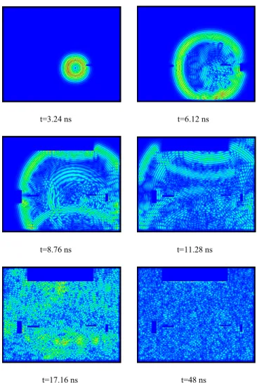
We precise the output points or plan where we need to get the fields values (‘txt’ files) or we can choose ‘PPM’ files to see how electromagnetic waves propagate inside the room for each time step “Fig. 3”. For this study we defined horizontal output plan as the same level of the source antenna.
After calculation of fields for each time and spatial steps in all the FDTD space, the code will produce for each point in the output plan the fields’ values in time domain.
t=3.24 ns t=6.12 ns t=8.76 ns t=11.28 ns t=17.16 ns t=48 ns
Fig. 3 Electromagnetic waves propagation in time domain (FDTD code)
Fig. 3 shows how electromagnetic waves propagate inside the office taking into account the presence of obstacles.
The calculation is done for 2000 time steps or the time step is 2.4 e-02 ns.
Another calculation is done to get the fields values in text files in order to compute the radiated power at 2.4 GHz to
compare between simulation and measurement results and validate this modeling.
The code produces the electromagnetic fields in time domain, then we need to use the Fourier transform to get the electromagnetic fields in frequency domain and extract the values of electric and magnetic fields at 2.4 GHz as shown in Fig. 4 in order to compute the Poynting vector P = | E x H | [15]. P = ( [(Ey.Hz) – (Ez.Hy)]2 + [(Ez.Hx) – (Ex.Hz)]2 + [(Ex.Hy) – (Ey.Hx)]2 ) 1/2 (W/m2) (1) (a) Fourier Transform (b)
Fig. 4 Ez from time domain to frequency domain: (a) Ez (V/m) in time domain (b) Fourier transforms of Ez (V/m).s
In our study we get the fields values for 93708 output points; we need to compare 143 positions with measurement values, the radiated power for these 143 points is computed and represented in Fig. 5.
The bleu areas show the influence of obstacles (computers, heater and wardrobes) on the radiation of antenna obtained by simulation with the FDTD code.
Fig. 5 Radiated power obtained with FDTD simulation (dBm) (The white area represents the wardrobes)
V. MEASUREMENTS
Two monopole omnidirectional antennas with the physical size of λ/4 (resonate at 2.4 GHz) are used in this scenario. The transmitting antenna is placed on the desk as shown in Fig. 6, the signal emitted is a CW signal using "Synthesized Signal Generator” which operates from 10 MHz to 20 GHz, the output power is 0 dBm, the received power is measured with a “Spectrum analyzer (9kHz-3GHz)”.
Fig. 6 Measurement of antenna radiated power in office environment
The repartition of radiated power measured for 143 positions separated by 30 cm at the same level of transmitting antenna is represented in Fig. 7.
To measure power for each position we select 8 discrete measurement points around the measurement position to get the average value. The distance of the discrete points is λ/2 from the measurement position.
Fig. 7 Radiated power obtained with measurements (dBm) (The white area represents the wardrobes)
Fig. 8 shows the difference between measurements and FDTD code results, a good agreement is obtained. To be precise, minor differences can be seen from -3 to 2.5 dB as shown in Fig.8, the biggest positive difference can be observed between the transmitted antenna position and the heater.
Fig. 8 Difference of radiated power (dB) between measurements and FDTD code results
VI. SIMULATIONWITHHFSS
The same scenario is realized with the commercial software HFSS 14.0 used for 3D full-wave electromagnetic field simulation based on the finite element method and the integral equation method. All the properties are respected (geometries, materials, positions, frequency, antenna). The simulations with HFSS produce the electromagnetic fields at all locations inside the room.
Fig. 9 shows the electric field distribution at 2.4 GHz.
Fig. 9 Electric field distribution at 2.4 GHz
The difference between HFSS results and measurements results can be seen from -12 to 12.75 dB. Fig. 10 shows that the biggest difference is observed between the computers.
Fig. 10 Difference of radiated power (dB) between measurements and HFSS results
VII. MODELINGANDMEASUREMENTSWITHOUT OBSTACLES
The same environment has been modeled without desks, wardrobes, computers and screens; we just kept the unmovable heater.
Fig. 11 (a-c) show the results obtained from FDTD code, HFSS and from measurements respectively.
The difference between the measurements and FDTD results is shown in Fig. 12 (b). Similarly the difference between the measurements and HFSS results is presented in Fig. 12 (b).
(a)
(b)
(c)
Fig. 11 Radiated power (dBm) obtained from: (a) FDTD results (b) HFSS results (c) Measurements results
The difference between the measurements results for the scenario with obstacles and without obstacles is shown in Fig. 12 (a) where the white area represents the wardrobes. This difference can be seen from -9 to 8 dB which show the influence of obstacles on the antenna radiation inside the office.
(a)
(b)
(c)
Fig. 12 Difference of radiated power (dB) between measurements without obstacles and: (a) Measurements with obstacles (b) FDTD code results
without obstacles (c) HFSS results without obstacles
The difference between FDTD code results and measurements results can be seen from -1.45 to 1.7 dB. The difference between HFSS results and measurements results can be seen from -18 to 13.5 dB.
VIII. COMPARISONBETWEENFDTDCODEAND HFSSSOFTWARE
The results of this study show a big difference of capability to modeling electromagnetic propagation in complex environment between the FDTD code and the commercial software HFSS.
In the FDTD study we used a normal computer which has four processors and 12 GB of memory (RAM), the scenario needs 2.25 GB of memory and we used just one processor to realize this computation.
The storage space that we used for this comparison for 143 output points is about 20 MB, but if we need to get all the points in the antenna level plan (93708 points) the storage space will be 12.7 GB, then it’s depending how much of accuracy we need to get.
In the HFSS study we used a powerful machine which has 16 processors and 96 GB of memory (RAM), the scenario needs 86.6 GB and all the processors to run this simulation. The storage space is about 3.2 GB.
TABLE I present computational comparison between both methods.
TABLE I. COMPUTATIONALCOMPARISON
METHOD Number of processors Real Time Computing Memory (RAM)
FDTD code 1/4 9h11 2.25 GB
HFSS 16/16 4h50 86.6 GB
IX. CONCLUSION
An accurate and efficient electromagnetic indoor propagation modeling based on the 3D FDTD method is developed and presented in this paper. This code takes into account the presence of obstacles.
Numerical results obtained in typical office environment at 2.4 GHz are compared with measurements results which show a good agreement.
The FDTD code is compared with the commercial software HFSS. There is a big difference in the computational performance efficiency of these methods. HFSS requires enormous computing resources; the FDTD code has the greater capability to modeling with accuracy this kind of environment.
To get more accuracy, the characteristics of antenna and the presence or movement of people should be integrated in the FDTD code.
REFERENCES
[1] Allen Taflove, Susan C. Hagness, Computational Electrodynamics: The finite-difference time-domain method, Artech House, Norwood, 2005.
[2] Yee K, “Numerical Solution of Initial Boundary Value Problems Involving Maxwell’s Equations in Isotropic Media”, IEEE Trans. Ant. Prop., vol. 33, May 1966, pp.302-307.
[3] Taflove A and Brodwin M, “Numerical solution of steady state electromagnetic scattering problems using the time dependent Maxwell’s equations”, IEEE MTT, vol. 23, no. 1, Aug. 1975, pp. 623-630.
[4] D Sheen, S Ali, M Abouzahra, and J Kong, “Application of Three-Dimensional Finite-Difference Method to the Analysis of Planar Microstrip Circuits”, IEEE MTT, vol. 38, pp. 849-57, Jul 1990. [5] X Zang, J Fang and K Mei, “Calculations of the dispersive
characteristics of microstrips by the FDTD method”, IEEE MTT, vol. 26, pp. 263-267, Feb. 1988.
[6] Railton C and McGeehan, “Analysis of microstrip discontinuities using the FDTD method”, MWSYM 1989, pp. 1089-1012.
[7] Shibata T, Havashi T and Kimura T, “Analysis of microstrips circuits using three-dimensional full-wave electromagnetic field analysis in the time-domain”, IEEE MTT, vol. 36, pp. 1064-1070, Jun. 1988. [8] Feix N, Lalande M and Jecko B, “Harmonically Characterization of a
Microstrip Bend via the FDTD Method”, IEE Proceedings, IEEE MTT, vol. 40, no. 5, May 1992, pp. 955-961.
[9] A Taflove, “The Finite-Difference Time-Domain Method for Electromagnetic Scattering and Interaction Problems”, IEEE Trans. Electromagnetic Compatibility, vol. EMC-22, pp. 191-202, Aug. 1980.
[10] Railton CJ, Richardson KM, McGeehan JP and Elder KF, “The Prediction of Radiation Levels from Printed Circuit Boards by means of the FDTD Method”, IEE International Conference on Computation in Electromagnetics, Savoy Place, London, Nov. 1991.
[11] WJ Buchanan, NK Gupta, “Prediction of Electric Fields from Conductors on a PCB by 3D Finite-Difference Time-Domain Method”, IEE’s Engineering, Science and Education Journal, Aug. 1995.
[12] Hese J and Zutter D, “Modelling of Discontinuities in General Coaxial Waveguide Structures by the FDTD-Method”, IEEE MTT, vol. 40, Mar. 1992.
[13] Paul D, Pothercary and Railton, “Calculation of the Dispersive Characteristics of Open Dielectric Structures by the FDTD Method”, IEEE MTT, vol. 42, no. 7, Jul. 1994.
[14] A. Taflove, Computational Electrodynamics The Finite-Difference Time-Domain Method. Boston: Artech House, 1995.
[15] Perambur S. Neeakanta, Theresa Kishkan, Rajeswari Chaterjee, “Antennas for Information Super Skyways: An Exposition on Outdoor and Indoor Wireless Antennas”, Reaserch Studies Press Ltd, pp. 223, 1st edition (December 1, 2002).