Model-free control of automotive engine and brake for Stop-and-Go scenarios

HAL Id: inria-00395393

https://hal.inria.fr/inria-00395393

Submitted on 15 Jun 2009

HAL is a multi-disciplinary open access

archive for the deposit and dissemination of

sci-entific research documents, whether they are

pub-lished or not. The documents may come from

teaching and research institutions in France or

abroad, or from public or private research centers.

L’archive ouverte pluridisciplinaire HAL, est

destinée au dépôt et à la diffusion de documents

scientifiques de niveau recherche, publiés ou non,

émanant des établissements d’enseignement et de

recherche français ou étrangers, des laboratoires

publics ou privés.

Model-free control of automotive engine and brake for

Stop-and-Go scenarios

Sungwoo Choi, Brigitte d’Andréa-Novel, Michel Fliess, Hugues Mounier, Jorge

Villagra

To cite this version:

Sungwoo Choi, Brigitte d’Andréa-Novel, Michel Fliess, Hugues Mounier, Jorge Villagra. Model-free

control of automotive engine and brake for Stop-and-Go scenarios. European Control Conference

(ECC’09), EUCA - IFAC - IEEE CS, Aug 2009, Budapest, Hungary. �inria-00395393�

Model-free control

of automotive engine and brake for Stop-and-Go scenarios

Sungwoo CHOI

, Brigitte d’ANDR ´

EA-NOVEL, Michel FLIESS, Hugues MOUNIER, Jorge VILLAGRA

Abstract— In this paper we propose a complete strategy for the longitudinal control of automotive vehicles in Stop-and-Go situations. Firstly, a upper level grey-box torque control is proposed to compensate for neglected dynamics at chassis level (due for example to road slopes, aerodynamic forces, rolling resistance forces, etc.). Secondly, to obtain the desired torque, we have considered a model-free approach to elaborate the suitable low level engine or braking torque. Convincing simulation results are presented to validate our method.

Index Terms— Stop-and-Go, model-free control, inteligent PID controllers, numerical differentiation, robustness.

I. INTRODUCTION

Driving assistance systems like Adaptive Cruise Control (ACC) and Stop-and-Go have been extensively studied in recent years [17]. The former is devoted to inter-distance control in highways where the vehicle velocity remains quasi constant, whereas the latter is appropriate for vehicles driving in towns with frequent and sometimes hard stops and accelerations. The constraints of these two situations are quite different in terms of comfort, so they have often been treated as two distinct approaches. The authors of [9] propose a unique non-linear reference model and controller for both ACC and Stop-and-Go scenarios. However, their feedback terms are not sufficiently robust to tackle external disturbances such as road characteristics and aerodynamic forces. A grey-box control strategy was therefore proposed in [18] in order to compensate all the neglected dynamics.

In [9] the authors suppose that the reference acceleration generated by the model can be instantaneously applied to the following vehicle. However, the corresponding braking and accelerating torques are often difficult to obtain because of the uncertainty of the engine/brake models. Different approaches have been proposed to handle the nonlinear dynamics of engine and brake: input/output linearization [16], [15], fuzzy logic ([11], [7]) and sliding mode ([6], [19], [12]) have been proposed for engine and brake control. S. Choi and B. d’Andr´ea-Novel are at Mines ParisTech, CAOR-Centre de Robotique, Math´ematiques et Syst`emes, 60 bd. Saint Michel,

75272 Paris Cedex 06, France. sung-woo.choi@ensmp.fr,

dandrea@ensmp.fr

M. Fliess is at INRIA-ALIEN & LIX (CNRS,

UMR 7161), Ecole´ polytechnique, 91128 Palaiseau, France.

Michel.Fliess@polytechnique.edu

H. Mounier is at Institut d’ ´Electronique Fondamentale

(CNRS, UMR 8622), Universit´e Paris-Sud, 91405 Orsay, France.

Hugues.Mounier@ief.u-psud.fr

J. Villagra is at Departamento de Ingenieria de Sistemas y Au-tomatica, Universidad Carlos III, 28911 Leganes (Madrid), Spain. jvillagr@ing.uc3m.es

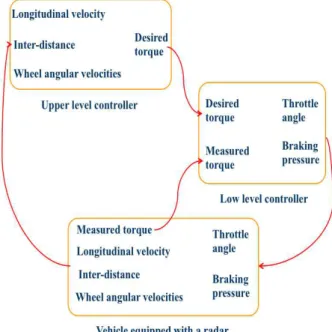
Fig. 1. General Stop-and-Go control scheme

Most of these methods use fixed gains, whereas the model parameters vary during the lifetime of the vehicle. In addition to this, off-line identification for an engine/brake modeling is often complex. We here propose a so called model-free control approach developed in [2], [3], which is inherently

robust to the very poorly known engine and brake dynamics.1

The remainder of the paper is organized as follows. The general control scheme is presented in Section II. In Section III we explain the model-free control setting. Section IV presents upper level control with the compensation of unmodeled dynamics using the so-called intelligent PID controllers [2], [3]. Section V is devoted to lower level engine/brake control and to associated simulations. A robust-ness study will be presented in Section VI.

II. CONTROL SCHEME

The whole control scheme is graphically summarized in Figure 1. The longitudinal control system architecture for the Stop-and-Go is designed to be hierarchical, with an upper level controller and a lower level controller. The upper level controller determines the desired torque for the vehicle

1_{See [8] for another application to the automotive industry, i.e., to the}

using longitudinal velocities, wheel angular velocities and inter-distance measurements by radar. An intelligent PID compensation is developed at this level to deal with the chassis dynamics uncertainties. The lower level controller determines the throttle angle input or the braking pressure input required to track the desired torque generated by the upper level controller. For the model-free control design, measured engine and brake torques are required as an input to this level. For the simulation, a 14 degree-of-freedom vehicle representation with tire models as well as a radar model have been used.

III. MODEL-FREE CONTROL2

We only assume that the plant behavior is well approx-imated in its operational range by a system of ordinary differential equations. The input/output equation looks like for a SISO system:

E(t, y, ˙y, . . . , y(ι),u,u, . . . , u˙ (κ)) = 0

where E is a sufficiently smooth function of its arguments.

Assume that for some integer n, 0 < n≤ ι, _{∂ y}∂ E(n) 6≡ 0. The

implicit function theorem yields then locally

y(n)= E(t, y, ˙y, . . . , y(n−1),y(n+1), . . . ,y(ι),u,u, . . . , u˙ (κ))

This equation becomes by setting E= F + αu:

y(n)= F + αu (1)

where

• α ∈ R is a non-physical constant parameter, such that

F andαu are of the same magnitude;

• the numerical value of F, which contains the whole

“structural information”, is determined thanks to the

knowledge of u,α, and of the estimate of the derivative

y(n) (see remark 1 below).

In all the numerous known examples it was possible to

set n= 1 or 2. If n = 2, we close the loop via the intelligent

PID controller, or i-PID controller,

u_{= −}F α+ ¨ y∗ α + KPe+ KI Z e+ KDe˙ (2) where

• y∗is the output reference trajectory, which is determined

via the rules of flatness-based control;

• e_{= y − y}∗ is the tracking error;

• KP, KI, KD are the usual tuning gains.

Remark 1: The numerical derivation of noisy signals, which is necessary to implement the feedback loop (2) is borrowed from [4] and already plays an important role in model-based control (see [10] for further important theo-retical developments, and, also, [1] for some applications). This approach obviously necessitates derivatives estimation

2_{See [2], [3] for more details.}

of noisy signals. The estimate of the 1st order derivative of

a noisy measured signal y can be expressed as follows: ˆ˙y = −_T3!3

Z T

0 (T − 2t)y(t)dt,

(3) where [0,T] is a quite “short” time window. Moreover, a filtered version of the noisy measured signal y yields:

ˆ y= 2! T2 Z T 0 (2T − 3t)y(t)dt. (4) The global structure of our scheme is the following: - the upper level uses an i-PD controller of the form (2) to

handle external disturbances (road slope, aerodynamic forces, ... see (12)). Equation (3) will also be used to estimate the time derivative of the inter-distance d which is necessary to obtain the leader vehicle velocity. - The lower level uses the other i-PD controllers (20) and

(22) to handle the unknown engine and brake dynamics. IV. UPPER LEVEL CONTROLLER

First of all, a short summary of the control law for the upper level controller is given and then the resulting engine/brake torque is elaborated.

A. Feedforward control

An inter-distance reference model proposed by [9] will act as a feedforward control law for the upper level controller. The inter-distance reference model describes a virtual vehicle

dynamics which is positioned at a distance dr (reference

distance) from the leader vehicle. The reference model dynamics is given by

¨

dr= ¨xl− ¨xrf (5)

where ¨x_l is the leader vehicle acceleration and the follower

vehicle acceleration ¨

xr_f = ur_(dr_{, ˙d}r_{) (6)}

is a nonlinear function of the inter-distance reference dr and

of its time derivative ˙dr_.

Introducing ˜d , d0−drin (6), where d0is the safe nominal

inter-distance, the control problem consists in finding a

suitable control when ˜d >0 so that all the solutions of

the dynamics (5) fulfill the following comfort and safety constraints:

• dr> dc, with dc the minimal inter-distance, will

guar-antee collision avoidance.

• k ¨xr_{k 6 B}

max, where Bmax is the maximum attainable

longitudinal acceleration, depending on the driver, the vehicle and the infrastructure, will have an effect on security and comfort.

• k...xr_{k 6 J}

max, where Jmaxis a bound on the driver desired

jerk, which directly affects the comfort performances. The work by [9] proposed to use a nonlinear damper model:

which leads to the following equation: ¨˜

d_{= −c| ˜}d_|d˙˜_{− ¨x}l.

The previous equation can be analytically integrated and

expressed in terms of dr_{, assuming that ˙x}

l(0) = 0: ˙ dr=c 2(d0− d r₎2_{+ ˙x} l(t) − β , β = ˙xrf(0) + c 2(d0− d r₍₀₎₎2 . (7) From (6), the feedforward control law is then obtained:

ur= ¨xr_{= c|d}

0− dr| ˙dr (8)

where the reference inter-distance evolution comes from numerical integration of (7). Note that the parameters c and

d0 are algebraic functions of comfort and safety parameters

(see [9] for details).

Remark 2: The leader vehicle velocity ˙xl is estimated

using ˙xl = ˙d+ ˙xf where ˙d is estimated by (3) from the

measured distance d.

B. Upper level closed loop control

The feedforward control should be corrected with feed-back terms which can compensate errors induced by mea-surement noises and external disturbances. We use an

alge-braic PD compensator3, so that the corrected acceleration of

(8) is given by:

u(= γx) = ur+ KPe+ KDe˙ (9)

where e represents the error between the real inter-distance

and the reference inter-distance ( e= d − dr _{), and its time}

derivative will be estimated using (3).

C. Engine/Brake torque generation

The wheel rotation dynamics can be written as follows:

I ˙_{ω = −rF}x+ τea− τba (10)

where I is the rotation inertia moment,ω is the wheel angular

velocity, r is the tire radius, Fx is the longitudinal tire force,

τea is the applied engine torque, andτba is the applied brake

torque, both of them applied at the wheel center.

The sum of the 4 wheels rotation dynamics equations and

of the vehicle longitudinal dynamic equation Mγx= ∑4i=1Fxi

yields τg= I 4

∑

where τg = τe− τb= ∑4i=1(τeai− τbai) is the generalized

total torque, M is the total weight of vehicle and γx is the

longitudinal acceleration. ˙ω is computed once more with (3)

from the measured wheel angular velocities.

Our final reference torque τg can be obtained using (11)

whereγx= u is given by (9), and an intelligent PID

compen-sation is applied to handle unmodeled external disturbances

γ0 (due to road slope, rolling resistance, wind, etc.):4

3_{See [5] for details.}

4_{See [18] for details.}

TABLE I

ENGINE MODEL VARIABLES AND PARAMETERS

˙

mace Mass air flow rate into the manifold (kg/s)

˙

macs Mass air flow rate out of the manifold (kg/s)

Pad Manifold pressure (Pa)

αp Throttle angle (◦)

wm Engine speed (tr/min)

Tm Internally developed torque (Nm)

Tch Load torque (Nm)

Tchpert Shaft torque (Nm)

kp Manifold dynamic constant

kn Rotational dynamics constant

τg= I 4

∑

V. LOW LEVEL CONTROLLER

In the lower level controller, the throttle angle input and the brake pressure input are calculated in order to track the desired torque determined by the upper level controller. For this study, an engine model and a brake model have been used.

A. Engine model

The engine model we use in this study was derived by Powell et al. [14] from steady-state engine maps. The model represents a 1.6 liter, 4-cylinder fuel injected engine. The dynamic equations of the model are:

˙ P_ad = kp( ˙mace− ˙macs) (13) ˙ wm = kn(Tm− Tch) ˙ mace = (1 + a1αp+ a2αp 2_)g(P ad) (14) g(Pad) = ( 1, Pad≤ 50.66 a3 q (a4Pad− P_ad2), Pad>50.66 ˙ macs = a5wm+ a6Pad+ a7wmPad+ a8wmP 2 ad Tm = a9+ a10meas+ a11wm+ a12w 2 m (15) e mas = ˙ macs 120wm (16) Tch = ( wm 263.17) 2_{+ T} chpert. (17)

All the quantities in those equations are explained in Table I

and we will use all the coefficients (ai, i= 1, ..., 12) proposed

in [13]. Tm is related to τg through the transmission chain

B. Brake model

We will use a simple brake model proposed in [19] where the brake hydraulic dynamics have been approximated by a linear second-order system. The dynamic equations for the brake pressure is:

˙z1 = z2

˙z2 = −b1z1− b1z2+ b3Pm (18)

Pω = z1

where Pm is the input to the solenoid valve and Pω is the

brake pressure at the wheel.

The brake torque τb is considered to be proportional to

the brake pressure at the wheel: τb= KbPω.

where Kb is the lumped gain for the entire brake system.

C. Model-free feedback control

Inspired by (1) with n= 0, we assume that there is locally

a linear relation between the measured engine torque and the throttle angle:

τe= kaαp+ G(t) (19)

where ka is a constant and G(t) represents neglected

dynamics of the engine. If we use as a throttle input:

αp=

1

ka

(a( ˙τe− ˙τg) + τg− ˆG), (20)

where a∈ R−,τeis the measured engine torque, and ˆGis the

estimate of G(t) which can be obtained from (19) in discrete time form:

Gk= τek− kaαk₋₁,

this control law leads to the following torque error dynamics:

a( ˙τe− ˙τg) − (τe− τg) = 0.

Thereforeτe will converge exponentially toτg.

The brake torque can also be expressed by:

τb= kbPm+ D(t) (21)

where kbis a constant and D(t) represents neglected

dynam-ics of the brake. And the same technique can be applied for the brake input too:

Pm=

1

kb

(b( ˙τb− ˙τg) + τg− ˆD), (22)

where b∈ R−_{,τbis the measured brake torque and ˆDis the}

estimate of D(t).

Remark 3: In (20) and (22), we need torque ments. From a practical point of view, the torque measure-ment is not an easy task. Instead, it could be estimated using (11). In order to test this, realistic noises have been

added on both angular wheel velocities ω and longitudinal

accelerations γx. To attenuate the perturbation due to these

measurement noises, αp and Pm are finally filtered using

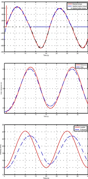
(4). Let us also notice that the time derivative terms in (20) and (22) are obtained using (3). Finally we have implemented our resulting control law which does not need any torque measurement but in absence of external dynamic disturbances on a typical Stop-and-Go scenario where several accelerations/decelerations are applied on a flat road. Figure 2 shows that the desired torque is pretty well tracked.

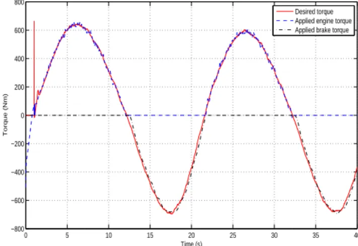
The same scenario is tested once more, with several external disturbances (road slope, rolling resistance and aerodynamic force) which are detailed for example in [18]. Thanks to the grey-box compensation on the upper level controller, external disturbances are efficiently compensated and the desired torque is well tracked too (see Figure

3). Indeed, in that case, we cannot obviously estimate γ0

from (12) if we suppose that the torque τg is not itself

measured. These simulation results show that our control strategy exhibits good robustness properties with respect to the external disturbances, if the torque is supposed to be measured.

VI. ROBUSTNESS STUDY OF THE MODEL-FREE CONTROL AGAINST PARAMETER VARIATIONS In order to show the robustness of our model-free control approach which does not rely on any parametric model, we can compare it with an analytical solution of the engine/brake models presented in Section V.

A. Analytical input solutions of the engine/brake models

Introducingmeas of (16) into (15) yields

Tm= A ˙macs+ B

A= a10

120wm, B= a9+ a11wm+ a12w

2

m. (23)

In a similar way, (23) can be rewritten using ˙macs from (13):

Tm= A( ˙mace−

˙

P_ad kp

) + B. (24)

If we rearrange (24) in terms of ˙maceand we compare it with

(14): ˙ mace= 1 A(Tm− B + A ˙ Pad kp ) = (1 + a1αp+ a2αp2)g(Pad)

then, the following second order equation in αp can be

written: aαp2+ bαp+ c = 0 a= a2, b= a1, c= 1 − Tm−B+A ˙ Pad kp Ag(Pad) . (25)

0 5 10 15 20 25 30 35 40 −800 −600 −400 −200 0 200 400 600 800 Time (s) Torque (Nm) Desired torque Applied engine torque Applied brake torque

5 10 15 20 25 30 35 20 25 30 35 40 Time (s) Inter−distance (m) Reference Real 0 5 10 15 20 25 30 35 40 12 14 16 18 20 22 24 26 Time (s) Velocity (m/s) Leader Follower

Fig. 2. Torques, inter-distances and velocities in a typical Stop-and-Go

scenario

Finally, we solve (25) and obtain a throttle angle input

which is a function of T m, Pad and ωm (the positive root

will be taken because physicallyαp≥ 0):

αp= f(Tm,Pad,wm) =−b +

√

b2_{− 4ac}

2a . (26)

For the brake input, we can express easily Pm from (18):

Pm=

1

b3

( ¨Pω+ b2P˙ω+ b1Pω) (27)

using algebraic estimates of ¨Pω and ˙Pω.

0 5 10 15 20 25 30 35 40 −1000 −800 −600 −400 −200 0 200 400 600 800 Time (s) Torque (Nm) Desired torque Applied engine torque Applied brake torque

5 10 15 20 25 30 35 −0.6 −0.4 −0.2 0 0.2 0.4 0.6 Time (s) External disturbances (ms −2) Road slope Rolling resistance Aerodynamic force 5 10 15 20 25 30 35 10 15 20 25 30 35 40 Time (s) Inter−distance (m) Reference Real

Fig. 3. Torques, external disturbances and inter-distance when the torque

is supposed to be measured

B. Influence of parameter uncertainties

We assume that parameters are not well known. We will

increase a9 and a10 up to 20 % in the engine model and b3

up to 20 % in the brake model. And then, we will compare the model-free control performance using [(20), (22)] with the analytical solution performance using [(26), (27)].

As the analytical solutions are obtained from (26) and (27), they are very sensitive to any parameter variation, and therefore torque tracking quality is quite poor (see Figure 4). On the contrary, the model-free control strategy shows good performances (see Figure 5).

5 10 15 20 25 30 35 40 −600 −400 −200 0 200 400 600 Time (s) Torque (Nm) Desired torque Applied engine torque Applied brake torque

Fig. 4. Influence of the parameter changes on the analytical solutions

VII. CONCLUSION

The model-free control approach has been applied to develop controllers in Stop-and-Go scenarios. Our control laws are naturally robust not only to unmodeled low level dynamics but also to external disturbances applied to the chassis. It should be pointed out that engine/brake torque measurements are no more needed and can be estimated using algebraic techniques in the disturbance free case.

REFERENCES

[1] S. Choi, B. d’Andr´ea-novel, J. Villagra, ‘Robust Algebraic Approach for Radar Signal Processing: Noise filtering, time-derivative estima-tion and perturbaestima-tion estimaestima-tion’ Proc. EU-Korea Conf. Science and

Technology, pp. 297-305, Heidelberg, 2008.

[2] M. Fliess, C. Join, ‘Commande sans mod`ele et commande `a mod`ele restreint’, e-STA, vol. 5, No 4, pp. 1-23. 2008. http://hal.inria.fr/inria-00288107/en/ [3] M. Fliess, C. Join, ‘Model-free control and intelligent PID

con-trollers: towards a possible trivialization of nonlinear control?’, Proc.

15th _{IFAC Symp. System Identif. (SYSID 2009), Saint-Malo, 2009.}

http://hal.inria.fr/inria-00372325/en/ [4] M. Fliess, C. Join, H. Sira-Ram´ırez, ‘Non-linear estimation is

easy’, Int. J. Model. Identif. Control, Vol. 4, pp. 12-27, 2008. http://hal.inria.fr/inria-00158855/en/ [5] M. Fliess, R. Marquez, E. Delaleau, H. Sira-Ram´ırez, ‘Correcteurs

proportionnels-int´egraux g´en´eralis´es’ ESAIM Control Optim. Calc.

Variat., Vol. 7, pp. 23-41, 2002.

[6] J.C. Gerdes, J.K. Hedriek, ‘Vehicle speed and spacing control via coordinated throttle and brake actuation’, Control Eng. Practice, Vol. 5, pp. 1607-1614, 1997.

[7] S. Germann, R. Isermann, ‘Nonlinear distance and cruise control for passenger cars’, Proc. Amer. Control Conf., Seattle, 1995.

0 5 10 15 20 25 30 35 40 −800 −600 −400 −200 0 200 400 600 800 Time (s) Torque (Nm) Desired torque Applied engine torque Applied brake torque

Fig. 5. Robustness of the model-free control against parameter changes

[8] C. Join, J. Masse, M. Fliess, ‘ ´Etude pr´eliminaire d’une

commande sans mod`ele pour papillon de moteur’, J.

europ. syst. automat., Vol. 42, pp. 337-354, 2008. http://hal.inria.fr/inria-00187327/en/ [9] J. Martinez, C. Canudas-de-Wit, ‘A Safe Longitudinal Control for

Adaptive Cruise Control and Stop-and-Go Scenarios’, IEEE Trans.

Control Syst. Techno., Vol. 15, pp. 246-258, 2007

[10] M. Mboup, C. Join, M. Fliess, ‘Numerical differentiation with anni-hiators in noisy environment’, Numer. Algor., Vol. 50, pp. 439-467, 2009.

[11] J. E. Naranjo, C. Gonz´alez, R. Garc´ıa, T. de Pedro, ‘ACC+Stop&Go Maneuvers With Throttle and Brake Fuzzy Control’, IEEE Trans. Intel.

Transport. Syst., Vol. 7, pp 213-225, 2006.

[12] L. Nouveli`ere, S. Mammar, ‘Experimental vehicle longitudinal control using a second order sliding mode technique’, Control Eng. Practice, Vol. 15, pp. 943-953, 2007.

[13] L. Nouveli`ere, ‘Commandes robustes appliqu´ees au contrˆole assist´e d’un v´ehicule `a basse vitesse’, Th`ese, Univ. Versailles - Saint-Quentin, 2002.

[14] B.K.Powel, D. Hrovat, ’Optimal idle speed control of an automotive engine’, Amer. Control Conf., Chicago, 2000.

[15] H. Raza, Z. Xu, B. Yang, P. Ioannou, ‘Modeling and control design for a computer-controlled brake system’, IEEE Trans. Control Syst.

Technol., Vol. 5, pp. 279-296, 1997.

[16] D. Swaroop, K. Hedrick, C. Chien, P. Ioannou, ‘Comparison of spacing and headway control laws for automatically controlled vehicles’,

Vehicle Syst. Dyn., Vol. 23, pp. 597-625, 1994.

[17] A. Vahidi, A. Eskandarian, ‘Research advances in intelligent collision avoidance and adaptive cruise control’, IEEE Trans. Intel. Transport.

Systems, Vol. 4, pp 143-153, 2003.

[18] J. Villagra, B. d’Andr´ea-Novel, M. Fliess, H. Mounier,

‘Robust grey-box closed-loop stop-and-go control’,

Proc. IEEE Conf. Decision Control, Cancun, 2008. http://hal.inria.fr/inria-00319591/en/ [19] K. Yi, J. Chung, ‘Nonlinear Brake Control for Vehicle CW/CA