Comparison of the tests chosen for material parameter identification to predict single point incremental forming forces

COMPARISON OF THE TESTS CHOSEN FOR MATERIAL

PARAMETER IDENTIFICATION TO PREDICT SINGLE POINT

INCREMENTAL FORMING FORCES

C. Bouffiouxc, C. Henrardd, P. Eyckense, R. Aerensf,A. Van Baele, H. Solg, J. R. Duflouh and A.M. Habrakend

c Department MEMCg currently ind d Department ARGENCO

Université de Liège, Chemin des Chevreuils 1, B-4000 Liège, Belgium

E-mail: chantal.bouffioux@ulg.ac.be, Christophe.Henrard@ulg.ac.be and Anne.Habraken@ulg.ac.be, Web page: http://www.argenco.ulg.ac.be

e Department MTM

Katholieke Universiteit Leuven, Kasteelpark Arenberg 44, B-3001 Heverlee, Belgium E-mail: philip.eyckens@mtm.kuleuven.be and Albert.VanBael@mtm.kuleuven.be,

Web page: http://www.mtm.kuleuven.be

f SIRRIS, Celestijnenlaan 300C, B-3001 Heverlee, Belgium E-mail: Richard.Aerens@sirris.be, Web page: http://www.sirris.be

g Department MEMC

Vrije Universiteit Brussel, Pleinlaan 2, B-1050 Brussels, Belgium E-mail: hugos@vub.ac.be, Web page: http://www.vub.ac.be/memc

h Department Mechanical Engineering

Katholieke Universiteit Leuven, Celestijnenlaan 300B, B-3001 Heverlee, Belgium E-mail: joost.duflou@mech.kuleuven.ac.be, Web page: http://www.mech.kuleuven.be/pma Keywords: Sheet metal forming, SPIF process, Inverse method, FEM simulations, Aluminum alloy AA3103

ABSTRACT. Single Point Incremental Forming is a sheet forming process that uses a smooth-ended tool following a specific tool path and thus eliminates the need for dedicated die sets. Using this method, the material can reach a very high deformation level. A wide variety of shapes can be obtained without specific and costly equipment. To be able to optimize the process, a model and its material parameters are required. The inverse method has been used to provide material data by modeling experiments directly performed on a SPIF set-up and comparing them to the experimental measurements. The tests chosen for this study can generate heterogeneous stress and strain fields. They are performed with the production machine itself and are appropriate for the inverse method since their simulation times are not too high.

1. INTRODUCTION

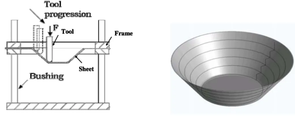
Single Point Incremental Forming (SPIF) is a new sheet metal forming process adapted to both rapid prototyping and small batch production at low cost. A clamped sheet is deformed by a spherical tool following a specific tool path (Figure 1) defining the final required shape without the need of costly dies. A wide variety of shapes can be made [1].

Sheet Frame Tool Sheet Sheet Frame Frame Tool Tool

Figure 1. Single point incremental forming machine and an example of a cone.

Accuracy of the FEM simulations of this process depends both on the constitutive law and the identification of the material parameters. A simple isotropic hardening model is not sufficient to provide an accurate force prediction [2].

A specific inverse method has been studied to provide the materials parameters using the results of experiments performed directly on a SPIF machine.

The material is an annealed aluminum alloy AA3103-O. A first set of material parameters, adjusted by the inverse method using classical tests (tensile and cyclic shear tests) is compared with a new set of data adjusted by both a tensile test and an indent test performed with the actual SPIF equipment.

To validate the material data sets, the evolution of the predicted tool force during a line test is compared with the experimental results. The F.E.M. code "Lagamine" and its inverse method code "Optim" have been both developed at the University of Liège.

2. MATERIALS 2.1. Material chosen

The SPIF process can be used with different alloys such as aluminum, titanium, copper and steel. This article focuses on the aluminum alloy AA3103-O, similar to AA3003-O. This annealed material was used in samples with a thickness of 1.5 mm.

2.2. Constitutive law

The elastic range is described by Hooke’s law where the Young’s modulus E= 72600 MPa and the Poisson’s ratio ν= 0.36 were identified using an acoustic method.

The plastic part is described by the Hill’48 law:

[

]

where the parameters F, G, H, and N, and the yield stress σF are identified using tensile

tests at 0°, 45°, and 90° from the rolling direction.

In the finite element code used, different kinds of hardening laws are available. In case of an isotropic hardening, the Swift law is given by:

(2) n p 0 F = K(ε + ε ) σ

where εp is the plastic strain, and K, ε₀, and n are the material parameters.

To use a kinematic hardening law, the stress tensor in (1) is replaced by σ−X where X is the back-stress. The material is assumed to have the same behavior in tension and in compression at the beginning of the process, so no initial back-stress is defined.

The evolution of the back-stress can be described by two formulations. The first one, Armstrong-Frederick’s equation, is:

) X . . X ( C X p p SAT X ε −ε = _& & & (3)

where CX is the saturation rate, XSAT is the saturation value of the kinematic hardening and

p

ε& is the anisotropic equivalent plastic strain rate. The second formulation, Ziegler’s hardening equation, is:

p A p F A ( X) G X 1 C X σ− ⋅ε − ⋅ ⋅ε σ = & & & (4) where CA is the initial kinematic hardening modulus and GA is the rate at which the

kinematic hardening modulus decreases with an increasing plastic deformation. This hardening equation is also available in Abaqus.

Minty’s law [3] is also used to explore the impact of texture. This law is based on a local yield locus approach able to predict texture evolution during FE modelling of industrial forming processes. With this model, only a small zone of the yield locus is computed. This zone is updated when its position is no longer located in the part of interest in the yield locus or when the yield locus changes due to texture evolution.

This model is specific in the sense that it does not use a yield locus formulation either for plastic criterion or in the stress integration scheme. A linear stress-strain interpolation in the 5-dimensional (5D) stress space is used at the macroscopic scale:

u C c _• τ = σ (5)

In this equation, σ is a 5D vector containing the deviatoric part of the stress; the hydrostatic part being computed according to an isotropic elasticity law. The 5D vector u is the deviatoric plastic strain rate direction (it is a unit vector), the macroscopic anisotropic interpolation is included in matrix C. τc _{is a scalar describing an isotropic work hardening at}

the microscopic level according to:

n 0 *

c_{=K .(Γ +Γ)}

τ ₍₆₎

The micro-macro model uses Taylor’s assumption of equal macroscopic strain and microscopic crystal strain. It computes the average of the response of a set of representative crystals evaluated with a microscopic model taking into account the plasticity at the level of the slip systems. The rate insensitive Full Constraints (FC) Taylor's model is used at the microscopic level.

The relations between these new material data and the macroscopic stress-strain curve parameters K, ε0, and n are:

1 n * M K K = ₊ (7) M . 0 0 _=ε Γ ₍₈₎

where M is the average of Taylor’s factor for a tensile test along the rolling direction. 2.3. Material data identification by inverse method

The inverse method is used to fit material data. This method, coupled with a Finite Element code, can be used to determine several parameters of a complex material law. The principle of this method is to choose a set of tests the results of which are sensible to the material data to adjust. These tests are simulated using an initial set of data, chosen arbitrarily – the better this initial guess is, the faster the method is. Then, the numerical results are compared with the experimental measurements and, using an optimization algorithm, the material data are iteratively adjusted until a sufficient accuracy is reached. The advantage of this method is the possibility of choosing a complex test to fit the parameters, inducing heterogeneous stress and strain states close to the ones reached during the process needed to be simulated with this material model.

3. EXPERIMENTAL PROCEDURE 3.1. Classical tests

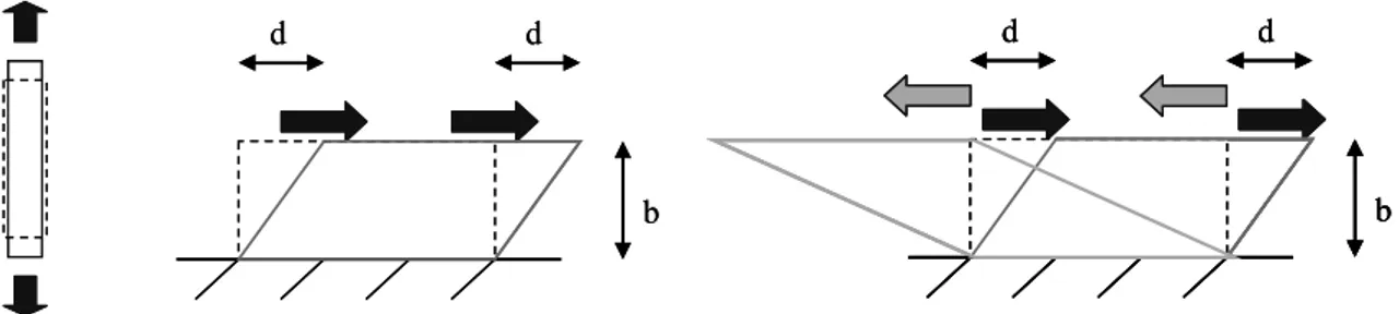
The first identification method consists of performing tests classically used to fit the material data of both the Swift law and the kinematic hardening. The tests chosen for this study are a tensile test, a monotonic shear test and two Bauschinger shear tests at two different levels of pre-strain Gamma = d/b = 10 and 30%, as illustrated in Figure 2.

d d b d d b d d b d d d d bb

Figure 2. Description of the classical tests: tensile, shear and Bauschinger tests.

3.2. Line test

A line test performed with the SPIF set-up is used to verify the accuracy of the fitted data: a square sheet with a thickness of 1.5 mm is clamped along its edges (Figure 3). The spherical tool radius is 5 mm. The tests are performed three times and the bolts of the frame are tightened using the same torque to ensure the reproducibility of the results.

The displacement of the tool is composed of five steps with an initial position tangent to the top surface of the sheet: a first indent of 5 mm (step 1), a line movement at the same depth along the X axis (step 2), then a second indent up to the depth of 10 mm (step 3) followed by a line at the same depth along the X axis (step 4) and the unloading (step 5).

The first step of this test is also used in the inverse method to determine accurate material data.

4. RESULTS

4.1. Data identification by classical tests

The tests described in section 3.1. are used to determine the material data by the inverse method using brick elements (Table 1). For the first set of data, the Swift law was coupled with the Armstrong-Frederick kinematic hardening for a Hill yield locus. Both Cx and Xsat are

equal to zero, which indicates that no kinematic hardening occurs. Such parameters give a good correlation between the experimental and simulation results (Figure 4).

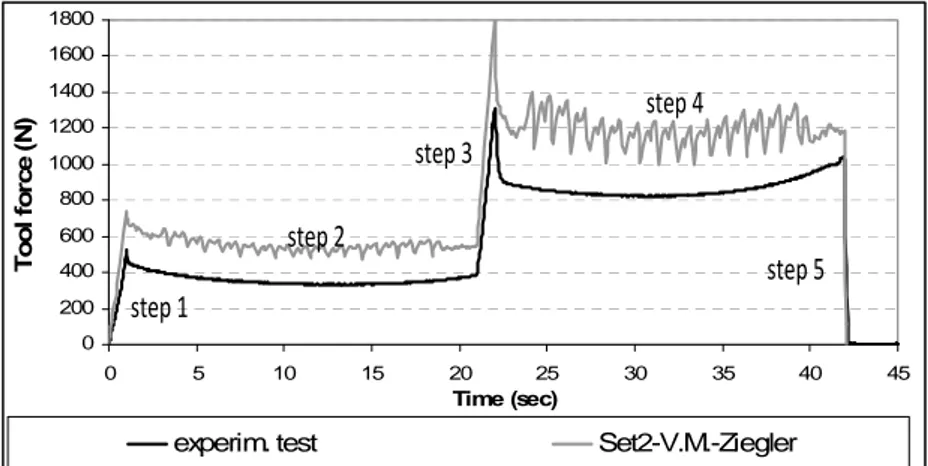
For the second set of data, the Von Mises yield locus was coupled with the Ziegler hardening in order to use the same law as in Abaqus. Unlike with the first set, this combination predicts kinematic hardening and provides a good prediction of experimental results except for the tensile test (Figure 5). In conclusion, it is observed that such tests do not indicate clearly whether kinematic hardening occurs.

Table 1. Data adjusted by classical tests (Units: N, mm)

Yield surface coefficients Swift parameters Back-stress data Set 1 HILL classic Isotropic hardening F= 1.224 G= 1.193 H= 0.8067 N= L= M= 4.06 K= 183 ε0= 0.00057 n= 0.229 Cx= 0 Xsat= 0 Set 2

Von Mises – Ziegler kinematic hardening F= G= H= 1 N= L= M= 3 K= 146.7 ε0= 0.0015 n= 0.229 CA= 240.6 GA = 11.2 Tensile 0 40 80 120 160 0 0.1 0.2 0.3 0.4 strain st re ss ( M P a)

Experimental set1-Hill classic

Shear 0 10 20 30 40 50 60 70 80 90 0 0.2 0.4 0.6 0.8 gamma str es s (M P a)

Experimental set1-Hill classic

2 Bauschinger 10% & 30% -80 -60 -40 -20 0 20 40 60 80 -0.6 -0.4 -0.2 0 0.2 0.4 gamma str es s (M P a)

Experimental set1-Hill classic

Tensile 0 40 80 120 160 0 0.1 0.2 0.3 0.4 strain str es s (M P a) Experimental set2-V.M.-Ziegler 2 Bauschinger 10% & 30% -80 -60 -40 -20 0 20 40 60 80 -0.6 -0.4 -0.2 0 0.2 0.4 gamma str es s (M P a) Experimental set2-V.M.-Ziegler Shear 0 10 20 30 40 50 60 70 80 90 0 0.2 0.4 0.6 0.8 gamma st ress ( M P a) Experimental set2-V.M.-Ziegler

Figure 5. Experimental and numerical results obtained by set 2 (kinematic hardening).

For the tensile test, plastic deformations occur beyond the elastic limit of 33.1 MPa. 4.2. Line test with data identification by classical tests

The line test, described in section 3.2., is used to verify the accuracy of the tool force prediction and to examine the impact of kinematic hardening.

In the FEM simulations, the nodes along the edges are fixed. The tool force is computed using a static implicit strategy. A Coulomb friction coefficient of 0.05 is applied between the tool and the sheet. The mesh density results from a compromise between the number of elements and the accuracy. Two element types are tested: brick with three layers along the thickness and shell elements.

Figures 6 and 7 show that the predicted tool force is systematically higher than the experimental one. The levels of the tool force obtained by set 1 (isotropic hardening) and by set 2 (kinematic hardening) are similar. The "Shells improved & sliding" curve of Figure 6 is an attempt to reduce the force and to be closer to the experiment, as is explained in section 4.4.

The oscillations in the numerical models are due to the contact elements. A sensitivity analysis to the meshing has shown that, unlike the bricks, the shell elements predict the same tool force for both a coarse and a very fine mesh. Such elements are therefore more accurate and better adapted to the inverse method since the computation time is also lower than when using the brick elements.

0 200 400 600 800 1000 1200 1400 1600 1800 0 5 10 15 20 25 30 35 40 45 Time (sec) To ol f o rc e ( N )

experim. test Bricks Shells Shells improved & sliding

step 2  step 1 

step 3

step 4

step 5 

0 200 400 600 800 1000 1200 1400 1600 1800 0 5 10 15 20 25 30 35 40 45 Time (sec) T o o l fo rc e (N )

experim. test Set2-V.M.-Ziegler

step 2  step 1 

step 3

step 4

step 5 

Figure 7. Evolution of tool force during the line test obtained by set 2 (Lagamine)

4.3. Texture effect

This paragraph analyzes the effect of using a texture-based law on the prediction of the tool force during the beginning of the line test. This texture analysis [3] is performed with Minty’s law (interpolation stress strain approach based on Taylor micro-macro homogenization rule and crystal plasticity) with a hardening law described by equations 5 and 6. The initial texture was measured at half the sheet thickness and the final texture was evaluated at the inner layer by a Taylor model.

0 100 200 300 400 500 600 700 800 900 0 2 4 6_{Time (sec)}8 10 T o o l fo rc e (N ) 12

experim. test Bricks - Hill

Bricks - Minty - init.text. Bricks - Minty - text. evol. - 2000 Bricks - Minty - text. evol. - 500 Bricks - Minty - final text.

step 2  step 1 

Figure 8. Texture effect

The four new cases, compared in Figure 8, correspond to the initial texture without a texture evolution, the initial texture with a texture evolution computed with 500 or 2000 crystals and the final texture without a texture evolution.

The values of the average of Taylor’s factor M in equations 7 and 8 are respectively for the initial and final textures: 2.94827 and 3.03903. Minty’s law is only available with brick elements.

In conclusion, the texture analysis predicts a tool force higher than in case of Hill's law and is then not able to explain the difference in force prediction. A simulation based on another homogenization rule (self consistent approach, Lamel, Alamel) would probably improve the results from micro-macro computation [4].

4.4. Sensitivity study

Previous experimental tests performed on a sheet with a thickness of 1.2 mm showed that the line test is highly sensitive to sliding at the edges. The force was up to 35% lower when

the bolts were tightened without a sufficient torque. A numerical sensitivity analysis showed that a small sliding of about 0.08 mm of the edges could decrease the tool force by 16%.

Then, for the experiments in Figures 6, 7 and 8, careful clamping of the frame provided an average measured sliding of only 0.0125 mm. A new model with springs regularly distributed along the edges can take into account a translation of the boundaries in the plane of the sheet. The spring stiffness, fitted to reproduce the same sliding as in the real process, is 500.10³ N/mm, with two springs every mm.

The effects of the geometry inaccuracy of the sheet (dimension, thickness, flatness) and the tool (initial position, diameter), of the machine elasticity, of the force measurement, of the FEM parameters (elements stiffness, number of layers for the bricks), of the material data values and of the friction coefficient have also been examined. All of the imperfections inducing a force reduction are combined, with realistic values, in this new model. The thickness is 1.49 mm, the tool diameter is 9.99 mm, the first and second indents are respectively: 4.96 mm and 4.94 mm instead of 5 for both. The sheet is meshed using very small shell elements and the boundary conditions are adapted to take into account the fact that the frame (204 mm * 204 mm) is larger that the backing plate (182 mm * 182 mm). Young’s modulus and Poisson’s ratio are also slightly modified: 70000 MPa and 0.33.

The tool force of this model, called: “Shell improved & sliding” in Figure 6, shows a relatively small force reduction: in comparison with simulations using a coarse mesh and shell elements, no imperfection, no springs and a baking plate of 182 mm * 182 mm, the force reduction is 5.6 % both after the first indent and after the second indent.

Separately or combined, none of these parameters can explain the gap between the predicted and experimental forces. In conclusion, the simulation inaccuracy cannot be explained by these investigations.

4.5. SPIF process

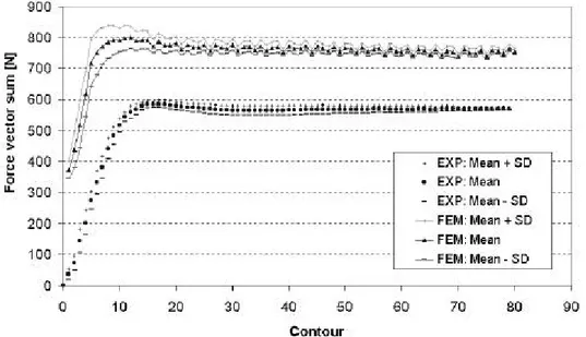
The simulation of the SPIF process (cone of Figure 1: 182 mm diameter, a sheet thickness of 1.2 mm, 40 mm depth, 50_degree wall angle) using such data allows another validation. As shown in [5] (Figure 9), the tool force prediction obtained with isotropic hardening is about 30% higher than the measurements.

Figure 9. Comparison between measured and predicted forces during the SPIF process

4.6. New data identification

The new identification method consists of fitting material data using both a classical tensile test (first test in section 3.1) and an indent test corresponding to the first step of the line test described in section 3.2. (Figure 10). The latter test contains heterogeneous stress and strain fields with tension, compression and shear stresses. The obtained material parameters are expected to be more accurate, since the deformation fields are much closer to those occurring in the SPIF process [6].

Figure 10. Description of the new tests chosen for the data identification. Tensile 0 20 40 60 80 100 120 140 160 180 0 0.1 _strain 0.2 0 S tr ess ( M p a) .3 exp. set3-Hill-A.F. set4-V.M.-Ziegler

Indent 0 100 200 300 400 500 600 0 0.2 0.4 0.6 0.8 1 Time (s) F o rc e (N )

exp. set3-Hill-A.F. set4-V.M.-Ziegler

Figure 11. Numerical and experimental results of the new tests: tensile and indent tests.

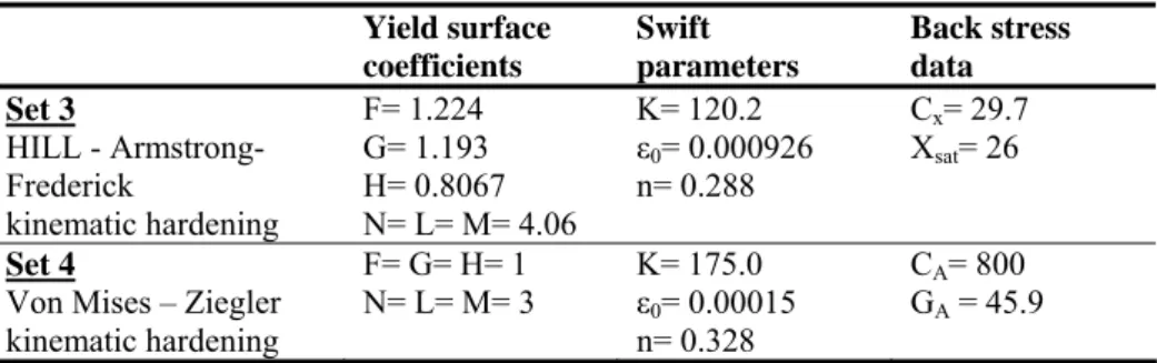
Table 2. Data adjusted by new tests (Units: N, mm) Yield surface coefficients Swift parameters Back stress data Set 3 HILL - Armstrong-Frederick kinematic hardening F= 1.224 G= 1.193 H= 0.8067 N= L= M= 4.06 K= 120.2 ε0= 0.000926 n= 0.288 Cx= 29.7 Xsat= 26 Set 4

Von Mises – Ziegler kinematic hardening F= G= H= 1 N= L= M= 3 K= 175.0 ε0= 0.00015 n= 0.328 CA= 800 GA = 45.9

Figure 11 shows a poor fitting in tension but a good force prediction in the indent test. Table 2 defines the parameter values fitted for both hardening models described in section 2.2. The simulations are performed using brick elements. Once again, the Ziegler hardening is coupled with the Von Mises yield locus in order to use the same law as in Abaqus.

Let us note that the onset of plastic deformation in tensile state is strongly modified: the elastic limit is 16.1 MPa for set 3 and 9.7 MPa for set 4. This difference induces a strong variation in the yield locus size as presented in section 4.8.

4.7. Line test with new data identification

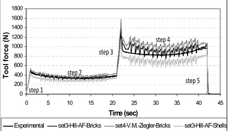
The two material models are used to simulate the line test with brick elements. Figure 12 shows a quite good correlation between the levels of predicted and measured tool forces, especially for the first two steps of the line test.

The simulation using shell elements predicts a lower tool force than with bricks. This comparison indicates that the material data are dependent on the stiffness of the element used. A new identification should be performed with the shell element.

0 200 400 600 800 1000 1200 1400 1600 1800 0 5 10 15 20 25 30 35 40 45 Time (sec) Too l for ce ( N )

Experimental set3-Hill-AF-Bricks set4-V.M.-Ziegler-Bricks set3-Hill-AF-Shells

Figure. 12. Evolution of tool force during the line test (Lagamine)

The comparison between Lagamine (home-made code by the MS²F – ARGENCO department) and implicit Abaqus FEM codes shows that, for the line test, the parameter identification depends on the hourglass stiffness of the reduced-integration brick elements.

The line test force prediction from Abaqus, using an hourglass stiffness of 1.33MPa, is about 80% that obtained with Lagamine. When an hourglass stiffness of 133MPa is used in Abaqus, the force prediction is around 800% of the Lagamine prediction.

4.8. Parameters validation by Abaqus

Since the Ziegler hardening coupled with Von Mises yield locus are available in both Lagamine and Abaqus, the parameters of set 2 in table 1 and set 4 in table 2 were used to simulate the classical tests with Abaqus using only one finite element. The results of the Lagamine code and Abaqus are exactly the same both for fully-integrated and reduced-integration elements. On the contrary, the results of the line test with Abaqus depend on the hourglass stiffness of the brick elements. This coefficient is not adjustable in Lagamine and by consequence, cannot be fitted in the model.

The use of the data specified in this paper requires thus the adjustment of this additional coefficient in Abaqus.

4.9. Yield locus shape

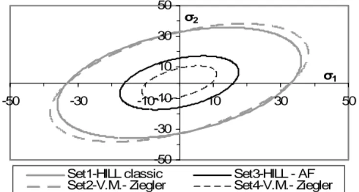
Figures 13 and 14 show the initial yield locus shapes and the yield locus at the end of the indent test in an element below the tool, for the four sets of material data (see tables 1 and 2).

-50 -30 -10 10 30 50 -50 -30 -10 10 30 50 σ1 σ2

Set1-HILL classic Set3-HILL - AF

Set2-V.M.- Ziegler Set4-V.M.- Ziegler

Figure 13. Initial yield loci in the principal stress directions for the different material models

-200 -150 -100 -50 0 50 100 150 200 -200 -150 -100 -50 0 50 100 150 200 σ1 σ2

Set1-HILL classic Set3-HILL - AF

Set2-V.M.- Ziegler Set4-V.M.- Ziegler

Element A

Figure 14. Yield loci in the principal stress directions at the end of step 1 of the line test in an element A located below the tool in the bottom layer for different material models

5. DISCUSSION

Figures 13 and 14 show that data fitted by the indent test induce kinematic hardening and a modification of the yield locus in compression but almost no adjustment in tension.

Our model did not introduce an initial back-stress as the annealed material is supposed to have the same initial behavior in tension and in compression. This assumption could be wrong but should require a physical explanation. A simple bending test has been performed, using an experimental set-up as described in [7], to verify this, but is not fully analyzed yet.

The shell elements having accurate results and a short computation time are more adapted to the inverse method than brick elements. The simulation by shell elements of the SPIF process should also give more accurate results. By consequence, the kinematic hardening and a remeshing adapted to shell elements has been recently implemented in Lagamine.

As a next step, the data can be fitted by tensile and indent tests using shells elements. The indentation depth can be increased or the whole line test could be used if a better data fitting is required.

6. CONCLUSIONS

The identification of material data is far from being trivial. The high strain state, reached during the chosen tests, have an important impact on the adjusted hardening material data and on the accuracy of the tool force prediction during the process.

The classical method used to identify material data by a combination of tensile and cyclic shear tests seems not adapted to the SPIF process on the aluminum alloy AA3103. Such tests give information in tension and in-plane shear only and the material is assumed to have the

same behavior in every direction.

On the contrary, our new approach based on tests inducing stress and strain fields similar to those present in the actual process predicts a better tool force. This heterogeneous strain field includes out-of-plane shear and in-plane compression, which is also present in the actual process: the line test and the SPIF process. The data adjusted by such a method give a better prediction of the global material behavior.

7. ACKNOWLEDGEMENTS

The authors of this article would like to thank the Institute for the Promotion of Innovation by Science and Technology in Flanders (IWT) and the Belgian Federal Science Policy Office (Contracts P6-24 and P2/00/01) for their financial support.

As Research Director, A.M. Habraken would like to thank the Fund for Scientific Research (FNRS, Belgium) for its support.

8. REFERENCES

1. J. Jeswiet, F. Micari, G. Hirt, A. Bramley, J. R. Duflou, J. Allwood: "Asymmetric Single Point Incremental Forming of Sheet Metal", CIRP Annals 2005, Vol. 54/2, Technische Rundschau, Switzerland (2005) 623-649.

2. P. Flores, L. Duchêne, C. Bouffioux, T.Lelotte, C. Henrard, N. Pernin, A. Van Bael, S. He, J. Duflou, A.M.Habraken: "Model Identification and FE Simulations: Effect of Different Yield Loci and Hardening Laws in Sheet Forming", International Journal of Plasticity, 23/3 (2007) 420-449.

3. A.M. Habraken, L. Duchêne: "Anisotropic Elasto-Plastic Finite Element Analysis using a Stress-Strain Interpolation Method based on a Polycrystalline Model", International Journal of Plasticity 20 (2004) 1525-1560.

4. L. Duchene, A.M. Habraken: "Multiscale approaches", Advances in Material Forming, Francisco Chinesta and Elias Cueto Editors, Springer (2007) 125-141.

5. S. He, A. Van Bael, P. Van Houtte, A. Szekeres, J.R. Duflou, C. Henrard, A.M. Habraken: "Finite Element Modeling of Incremental Forming of Aluminium Sheets", Advanced Materials Research 6-8 (2005) 525-532.

6. J.R. Duflou, J. Verbert, B. Belkassem, J. Gu, H. Sol, C. Henrard, A.M. Habraken: "Process Window Enhancement for Single Point Incremental Forming through Multi-Step Toolpaths" accepted for CIRP Annals-Manufacturing Technology, Vol. 57/1/2008.