Smoothing the TCP rate by learning the delay
versus window size dependency
Ibtissam El Khayat and Guy Leduc
Research Unit in Networking University of Li`ege
Institut Montefiore - B28 - Sart Tilman Li`ege 4000 - Belgique
Abstract. We propose TCP-L, an improved version of TCP, equipped with a learning algorithm whose purpose is to avoid probing for ad-ditional bandwidth when the network conditions are known to be un-favourable. TCP-L learns the relationship between its current (average) one-trip delay and its current window size when congestion occurs, lead-ing to packet loss. After the learnlead-ing phase, TCP-L will only probe for bandwidth by increasing its window if, under the current network con-ditions (measured by the one-trip delay), this inflated window has not previously created congestion. Simulations show that after the learning phase, TCP-L reaches a much more stable throughput, while remaining TCP-friendly, which makes it usable for a larger class of applications, including some multimedia applications that will benefit from that sta-bility. TCP-L is a simple backward compatible extension of TCP which can thus be deployed progressively. We show that there is a benefit for the Internet to deploy TCP-L, because the overall traffic becomes smoother when the proportion of TCP-L flows increases. Finally, our learning com-ponent can also be easily embedded in other unicast or multicast trans-port protocols.
1
Introduction
TCP has some useful properties that should be preserved. Its reliable transfer and its cooperation to avoid the collapse in case of congestion explain its success in the current network. TCP has evolved since 1988. Several phases have been added as the fast-retransmit and the fast re-covery, and several TCP variants have been created (e.g. New-Reno, TCP-Vegas, TCP-Sack).
Nevertheless, this protocol still has some weaknesses. A defect often pointed out (e.g. [4], [1], [10]) is the oscillation of the TCP window, which makes it ill-suited for real-time multimedia flows. Some protocols called model-based flow control (MFC) are based on a TCP model (e.g. [6], [5], [8]) which represents the throughput of a TCP flow as a function of packet loss and round trip time. The goal is to have a rate equal in average to the one of TCP. When a congestion occurs, the sender (or the receiver) computes the new rate it can get and reduces its rate accord-ingly. This reduction is not as drastic as dividing by 2 and it is more
bearable for the real-time multimedia application user. Other protocols (IIAD [1], SQRT [1], TEAR [11], SIMD [3], DWAI/LDMD [9]) have been developed for Real-time streaming applications with the objective of be-ing as smooth as possible. However, this kind of protocols fails to share fairly the network resources with TCP in case of high losses. This is due to the fact that the TCP additive window increase is more aggressive than the one of other protocols. To be as aggressive as TCP we need to maintain the additive increase. If we maintain it and we want to be TCP-Friendly we must also divide the congestion window size by two when a congestion occurs.
This oscillatory behaviour of TCP is due to the fact that it endlessly persists in attempting to increase its rate. This increase always ends by causing congestion which forces TCP to reduce its rate subsequently. Furthermore, this congestion can have an impact on other TCP flows sharing the bottleneck. They all reduce their rate and the links become underused. The problem is that this behaviour of growing up until con-gestion is periodic. So, TCP will continue to lose packets during the whole session and the links thus will be underused. Even when TCP does not share a link with any other traffic, it does not work at the maximum rate because of this dynamics. Every time it reaches the maximum, it tries to inflate its congestion window and this leads straightforwardly to packet loss and consequently to a decrease of the rate. In this paper, we want to simultaneously control the congestion, avoid unnecessary packet losses, stabilise the rate, and be TCP-Friendly. The idea of our proposal is to im-prove TCP by adding a capability to learn its maximal rate (not leading to congestion) depending on network conditions by endowing it with a memory that allows it to retain the maximum rate it has reached without congestion under some network conditions. So, with this memory, TCP will not probe anymore for more bandwidth if the inflated window has previously created congestion under the same network conditions. And, when the network conditions become better (more available bandwidth) it will probe. Note that this modification can be added to any MFC or any protocol probing for bandwidth by increasing the rate (e.g. CIFL [2]).
2
The protocol bases
2.1 The states of TCP
The state of a TCP sender at time t can be represented by a pair < Wt, Ct> where Wtand Ctare respectively the congestion window and
the network conditions at time t. At the reception of an acknowledge-ment, the sender has no choice. If it is not limited by the receiver window, the sender must inflate its window. Afterwards, two situations can occur: – TCP succeeds and then the sender reaches the state <Wt+ 1, Ct+1>
– The inflation causes congestion and then the sender has to divide its window by 2 (congestion avoidance). The state reached is then <(Wt+ 1)/2, Ct+1>. Or, the sender goes to a slow start phase and
TCP-L 3 w w + 1 2w 2w+1 2w+2 a1 a1 a1 a2 a2 a3 a3 a3 a3 a3 a2 = if loss a1 = if ack
a3 = if ack but increasing w is known to create congestion Fig. 1. State machine of TCP in congestion avoidance phase If we only consider the congestion avoidance phase, TCP can be pre-sented by the state machine illustrated in Figure 1 without the dashed loop. For more readability, we do not introduce the network conditions in the drawing.
2.2 Introduction of a new action
When a TCP sender in a state <Wt, Ct> receives an acknowledgement,
it has to inflate its congestion window and to wait for the consequences. However, if in the same network conditions Ct, a window size of Wt+ 1
has already caused congestion, it is useless for the sender to try to inflate its window (as it will certainly lead to a congestion). To avoid this, we propose to add two new abilities to TCP: first, a memory that allows it to retain the states <Wt, Ct> where it has noticed congestion in the past
and, second, the possibility to leave the window size unchanged when the sender receives an acknowledgement. This new action is illustrated in Figure 1 by the dashed loop. The sender now proceeds as follows. At the reception of an acknowledgement, it chooses to maintain its window size constant if it has already visited this state and failed in increasing its window. Otherwise, it increases its window size by one. On the other hand, when TCP loses a packet, it divides1 its window size by two but
it further keeps in its memory the information that the current state should not be visited anymore later.
We call this new TCP TCP-L (L for learner). Actually, this strategy can be seen as a simple form of reinforcement learning algorithm. In artificial intelligence, reinforcement learning algorithms are generic tech-niques that aim at giving a system the ability to improve its behaviour by taking account of its past successes and mistakes.
2.3 Network conditions
Until now, we have not defined the network conditions Ctyet. The
net-work conditions can be defined by the path followed by the packets and the length of the queues. So, over the same path, the network conditions can be defined with only the mean queuing delay between the sender and the receiver.
1 TCP will decrease its window size only if it loses packet, thus avoiding to be as
A legitimate question at this point is why do we not use the round-trip-time instead of the queuing delay between the sender and the receiver, especially since the round-trip-time is already computed at the sender side. In fact, imagine that TCP is stable for a certain time and that traffics decrease in the return path. The round-trip-time would decrease and the queuing delay from the sender to the sink would remain constant. If we base our protocol on round-trip-time estimation, the sender would increase unnecessarily its congestion windows, which would not be the case with the queuing delay.
2.4 Reduction of the state space
In section 2.4 and 2.5, we consider that the path does not change during the session. We can thus refer to the queuing delay to mean the network conditions. Since the queuing delay can take an infinite number of values, there are two problems with the strategy proposed in Section 2.2. First, it is impossible to store in memory an infinite number of forbidden states <Wt, Ct>. Second, TCP may have to wait for ages before exploring all
the possible states. To solve this problem, we could discretise the values the queuing delay can take, and possibly refine this discretisation if the interval of the queuing delay is short.
Instead, we choose another solution. Denoting by qdtthe queuing delay at
time t, we consider that if qdt< qdt0 then the network at time t0is more
loaded than at time t. So, when TCP fails in increasing its window size while being in state <W, qd>, it learns that it will also fail in increasing its window size from any state <W, qd0> where qd0> qd.
Thus, this property allows to greatly extend the space of visited states at each failure (a sort of pruning) and it is sufficient to retain a single value of the queuing delay for every possible value of the window size. If later, there is less traffic, the queuing delay will decrease and the system will reach a state which has never been explored. TCP will then inflate its window and will continue its growing up until it reaches a new congestion. Remark: Since the only operation using the queuing delays is a (relative) comparison, the non-synchronisation of the sender and the sink clocks is not considered as an issue because it does not affect the result of the comparison.
2.5 Graphical representation
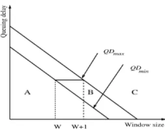
In state <w, qd> the TCP-L sender is faced with one of the three possi-bilities:
1. It is sending at the maximum rate allowed without creating conges-tion. It should maintain its congestion window size.
2. It is not sending at the maximum rate allowed. It can inflate its congestion window without causing any congestion.
3. It is sending too much data, and a congestion will occur.
The first case defines the operating area (B area in Figure 2). For each w the B area can be seen as an interval I = [QDmin, QDmax). If qd∈
[0, QDmin) then the sender is in the second case which is represented by
region A in Figure 2. We qualify this area as underused. The last case is associated with the forbidden area (C area in Figure 2). The sender is in
TCP-L 5 Window size Queuing delay QD QD max min W W+1 A B C
Fig. 2. The areas defined by the functions QDminand QDmax
this area if its queuing delay qd belongs to [QDmax,∞). QDmax(w) is
in fact equal to QDmin(w− 1).
The function QDmin : w 7→ QDmin(w) is decreasing (not inevitably
strictly). In fact, according to Mistra in [7], the TCP congestion window size W is equal to a certain (g(f (Q)))−1, where Q is the buffer occupancy and f (Q) the drop/marking function. The function g depends on the model used but it is always monotonic increasing, and f must never decrease to be meaningful. So W never increases when Q increases. See differently, if at time t the sender can inject up to w, and at t0can inject w + 1 without creating congestion then, the buffers were more loaded at t and thus the queuing delay at t0 is lower than the one computed at t. So Q, and thus both QDminand QDmax, are decreasing with w. For
simplification reasons, we choose a straight line to represent the curve of QDmin and QDmax in Figure 2. The two curves define the three areas
we talked about previously. The learning algorithm embedded in TCP-L finds points included in the operating area. Above these points, a TCP-L sender is necessarily outside the underused area and must not inflate its congestion window.
Remark: If for a given W , QDmaxis defined, a TCP-L sender should not
decrease its congestion window size even if its queuing delay increases significantly and enters region C, otherwise, it would get, like TCP-Vegas, less than its fair share compared to legacy TCP flows.
2.6 When the path changes
What we have proposed until now is valid only in the case of packets following one invariant path. If a new path is used when the sender is stable, the knowledge of TCP-L becomes obsolete, and could unneces-sarily constrain the sender to use small windows for example. When the path changes, the new QDmincurve could be in one of the 4 following
positions:
1. It could be between the two old curves QDminand QDmax.
2. It could be above the old QDmax.
3. It could be under the old QDmin.
4. It could cross the old QDmin and/or QDmax curves, but this case
can be considered as a combination of the other 3 cases.
We focus our explanation only on the case without packet loss, because when a packet is lost, the sender divides its congestion window size by 2 and would thus reach one of the previous three cases.
Case 1 Old Qdmax Case 3 3 1 2 3 2 1 1 2 3 Queuing delay Window size Old Qdmin New Qdmin Case 2 Queuing delay Window size Queuing delay Window size
Fig. 3. The three possible scenarios in the case of path change When the sender is stable before the path changes, it is necessarily in area 1 in the three graphs of Figure 3. We will explain each case in turn. Let W be the congestion window size at which the sender is stable.
Case 1
a. If the queuing delay increases but stays in area 1 which is the oper-ating area for the old path. The sender stays stable, but should not because it is in the new underused area.
b. If the queuing delay goes to area 2 or area 3, the sender, if it has its (W, QDmax(W )) defined, normally expects to lose packets.
See-ing that there is no loss, the sender understands that its path has changed.
Case 2
a. If the queuing delay increases but stays in area 1. We are in a situ-ation similar to 1.a.
b. If the queuing delay goes to area 2, there is no problem. The sender would be in the right place, in the operating area for the old and the new path.
c. If the queuing delay goes to area 3 we are in a situation similar to 1.b..
Case 3
a. If the queuing delay decreases and stays however in the area 1 with-out entering the forbidden region of the new path, the sender would remain rightly stable.
b. If the queuing delay goes to area 2, the sender thinking that it is in its underused region will try to inflate its congestion window and will lose packets. The sender will thus adjust its learning.
c. If the queuing delay goes to area 3 which is the underused one for both paths, the sender will increase its congestion window size until it causes congestion.
So if the sender is in case 3, it will always find the new QDmin curve.
For cases 1.b. and 2.c., if the point (W, QDmax(W )) exists, the sender
will discover that the path has changed favourably. But, in cases 1.a. and 2.a., if TCP-L relies only on the mean queuing delay it won’t discover that the path has changed. New mechanisms are then needed.
The queuing delay and the inter-packet delay dispersion can be used to discover that a path has changed. We have performed some experiments that show that the minimum, maximum, and standard deviation of the
TCP-L 7 queuing delay and of the inter-packet delay over one RTT are good indi-cators of path change. However, the derivation of a practical algorithm to detect topological changes in the network using these parameters clearly needs further investigation. One (quite classical) way to detect changes during the temporal evolution of some random variables is to assume that the values of these variables at each time step follow some probability dis-tribution whose parameters are estimated from previous observations of the variables. This probabilistic model is then used to derive confidence bounds on future values of the variables under the hypothesis that the network does not change. If the values of the variables at some time fall outside the confidence bounds, then it is claimed that a path change has occurred. The robustness of this simple algorithm could be improved by requiring several consecutive out-of-the-trend values before considering that there is really a path change.
Another mechanism can be added to discover a path change. If TCP-L has been stable for some round-trip-times then it can :
1. try to inflate its window even if it has failed before in the same or better conditions, or
2. send a kind of “trace-route packet” to see if the path has changed. If the first solution is adopted, the sender will probe for bandwidth reg-ularly and will succeed if the path has changed and is not overloaded. But this solution can disturb unnecessarily the stability reached, when the path has not changed. There is a trade-off between an implicit inves-tigation (as made by TCP and other protocols like the ones of [1]) and the stability. The second solution should be preferred for the stability it brings. With this solution, if the route changes, TCP-L will discover it and will forget what it has learnt. However, if the first solution is cho-sen, the sender should absolutely divide its window and not only return to the level it has just left. Indeed, to remain TCP-Friendly, a probing sender has to react to the congestion it causes like the other competing flows.
2.7 TCP Friendliness
A naive intuition could be: “if TCP-L increases its rate less frequently than TCP (due to action a3 of Figure 1) and reduces it in the same way it will not be able to cope with competing TCP”. This is true, but TCP-L only gets marginally less throughput than TCP. To understand this, consider a simple scenario where a TCP flow shares a bottleneck with a TCP-L flow. Suppose (fig. 4) that the two flows start at the same
Cycle W-1 W+1 TCP-L TCP Fig. 4. W := W/2 Cycle W TCP-L TCP Fig. 5. W := W/2 + 1
time (if it is not the case, we can show that they converge to this case after a while) and have the same RTT. Suppose that the bottleneck link can accommodate bursts up to 2W− 1 packets per RTT without loss. Figure 4 shows that TCP-L, after learning this limit (i.e. after a loss) will not increase its window above W− 1 while the competing TCP flow is present. By contrast TCP generates congestion when reaching W + 1 periodically, forcing both flows to divide their window in general. At steady state, the TCP rate is approximately 1 packet per RTT above the TCP-L rate. But note that the situation can be reversed easily by letting TCP-L reduce its window to W/2 + 1 after a loss (Figure 5 ), instead of W/2.
Although there may exist situations where TCP-L is more conservative than TCP (but not the opposite), none of our simulations have shown that.
2.8 Update of an existing TCP version
The transition from TCP to TCP-L is quite easy. We just need a one-dimensional array QD whose length is equal to the maximum congestion window. Each element QD[i] represents the lowest observed mean queu-ing delay leadqueu-ing TCP-L with window i to a loss. When TCP-L wants to increase its window it checks QD[i] to verify if the mean queuing de-lay it has just computed is below it. If it is below, TCP-L inflates its window, otherwise it maintains it constant. Because we need to measure the queuing delay from the sender to the sink, we can do almost all the modifications at the receiver side. And, when the receiver decides that the congestion window has to be maintained, it informs the sender that its window (flow control) is equal to the last congestion window size. An alternative way to upgrade TCP would be to modify the sender. Thus, because the senders are often servers, we can get very quickly many more TCP-L flows with fewer TCP stack upgrades. We do not activate the protocol if the window size is lower than 6. This is because TCP-L is activated only in the congestion avoidance phase. We explain in Table 1 the modifications we should add to TCP to get TCP-L without the mech-anism we talked about in section 2.6. These modifications can be added very easily to any existing TCP variant (Reno, New Reno, Tahoe ....).
3
Simulation results
For our simulations, we use NS2 and bring the modifications we talked about to TCP Reno. Traceroute is the only mechanism, useful when the route changes, that we have not implemented.
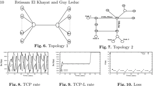
Comparison between TCP and TCP-L: We use, for this
pur-pose, Topology 1 (Figure 6) with n = 2 where two TCP traffics compete for 60s. Figure 8 shows the TCP rate oscillation which makes it unusable in the case of real-time multimedia applications.
When TCP-L is used instead of TCP, the link is used at 100%, and the traffics become smooth very quickly as seen in Figure 9. When we compare the number of packets lost in both cases (Figure 10), we see that
TCP-L 9 Table 1. The patch of an existing TCP version
– we create a function called ComputeMeanQdOverTheLastCwnd() which gives the last mean queuing delay. It is called from the receive function.
ComputeMeanQdOverTheLastCwnd() { if (loss) {
npack:=0 //number of packets sumQd:=0
return }
if (npack<cwnd) {
sumQd:+= Qd //Qd is the last packet queuing delay npack++ } if (npack==cwnd) { lastmeanQd:= sumQd/cwnd; npack=0; sumQd:=0; } }
– In function ”loss()” we add: QD[cwnd]:=lastmeanQd and
cwnd:=cwnd/2 may become cwnd :=cwnd/2 + 1
– at the reception of the last ack of the last previous window we add: if (QD[cwnd+1] exists && lastmeanQd >= QD[cwnd+1]) {
cwnd--; //cwnd was incremented by 1 }
TCP has cyclic losses where, after 5 seconds, TCP-L does not lose packets any more. Not losing packet avoids retransmission and especially avoids the useless reduction of rate. It is important to note that the protocols cited in the introduction, even when they are competing with themselves, continue to lose packets (See for example Figure 8 of [3]).
The last 20 seconds of Figure 9 show an important aspect of the protocol, which is its reaction in case of bandwidth availability. After 60 seconds in the previous experiment, we stop one of the two flows, the remaining one grows up very quickly to use all the bandwidth.
The effect of the round-trip-time : For TCP the proportion of unused
bandwidth increases when the round-trip-time increases because TCP takes more time to reach the problematic window size with long RTTs. The experiments performed in this section confirm it, and show that replacing TCP by TCP-L improves the usage of the bandwidth. We have run 3 TCP senders (Topology 1 with n=3) and have computed the proportion of the bandwidth used for different propagation delays. We
S1 S2 R1 R2 Sn Sn-1 Rn Rn-1 Fig. 6. Topology 1 R5 R2 R3 R4 S3 S2 S0 R1 Sink 3
Sink 0 Sink 1 Sink 2
1Mb,1ms 1Mb,50ms Fig. 7. Topology 2 0 200 400 600 800 1000 0 10 20 30 40 50 60 Bw (Kbps) Time (sec) S1 S2 Fig. 8. TCP rate 100 200 300 400 500 600 700 800 900 1000 0 10 20 30 40 50 60 70 80 Bw (Kbps) Time (sec) S1 S2 Fig. 9. TCP-L rate 0 2 4 6 8 10 12 14 16 18 0 10 20 30 40 50 60 # loss Time (sec) TCP-L TCP Fig. 10. Loss have done the same experiments in the case of 3 TCP-Ls. The results are illustrated in Table 2. In the case of TCP-L the link is used at 100% after the stabilisation without any packet loss whatever the propagation delay is.
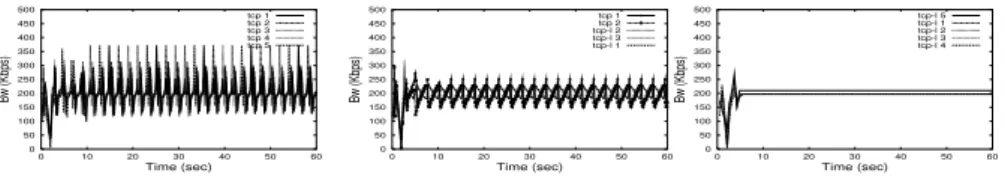
A slow transition : The goal of this section is to show that a slow
transition is possible and improves the quality of TCP itself. We use the topology of Figure 6 where n = 5, we connect each source Si to Ri. We begin by using 5 TCPs and then replace one TCP by one TCP-L at each experiment. We use this experiment only to show the bandwidth obtained by each flow. The results are shown in Figure 11. We can see that the rates of all flows become smoother when we increase the number of TCP-Ls.
To illustrate better what happens, we use the topology of Figure 6 with n = 10 and compute the loss ratio, the share ratio and also the goodput as a function of the number of TCP sources. The share ratio is the ratio between the mean TCP rate and the mean TCP-L rate. We run the simulations for 100 seconds. We can see on Figure 12(c) that the share remains quite stable and also that the loss ratio decreases when we increase the number of TCP-Ls. That means that TCP-Friendliness is satisfied and also that when we increase the number of TCP-Ls, ordinary TCP flows also get higher rates, and lower losses.
Path change : We use a topology where the sink is connected to
the sender through two paths (a and b). The flow follows path (a). Af-ter 15 seconds we force the flow to pass through (b) which offers higher bandwidth (1.2Mbps instead of 800Kbps) and equivalent queuing delay.
Table 2. The proportion of bandwidth used.
Propagation delay 10 100 200 300 400 500 TCP (over the whole session) 97.96 97.11 91.26 85.16 80.99 76.32 TCP-L(over the whole session) 99.19 98.36 96.00 92.78 91.17 86.57 TCP (After stabilisation) 98.71 98.67 94.16 90.69 87.94 85.31 TCP-L(After stabilisation) 100 100 100 100 100 100
TCP-L 11 0 50 100 150 200 250 300 350 400 450 500 0 10 20 30 40 50 60 Bw (Kbps) Time (sec) tcp 1 tcp 2 tcp 3 tcp 4 tcp 5 0 50 100 150 200 250 300 350 400 450 500 0 10 20 30 40 50 60 Bw (Kbps) Time (sec) tcp 1 tcp 2 tcp-l 2 tcp-l 3 tcp-l 1 0 50 100 150 200 250 300 350 400 450 500 0 10 20 30 40 50 60 Bw (Kbps) Time (sec) tcp-l 5 tcp-l 1 tcp-l 2 tcp-l 3 tcp-l 4
Fig. 11. Replacing more and more TCP flows by TCP-L flows.
0 0.5 1 1.5 2 2.5 3 0 2 4 6 8 1097 97.5 98 98.5 99 99.5 100 Loss rate (%) # TCP-L Loss efficiency
(a) Loss rate & efficiency
945 950 955 960 965 970 975 980 0 2 4 6 8 10 Bw (kbps) # TCP-L (b) Goodput 0 0.5 1 1.5 2 0 2 4 6 8 10 TCP-L/TCP # TCP-L (c) BW share ratio Fig. 12. The impact of replacing some TCP by TCP-L
Figure 13 (left) shows that when the TCP-L path changes, its rate in-creases and occupies the whole bandwidth even if its queuing delay has not changed. This is due to its minimum inter-packet delay which has decreased because the link capacity has increased.
Another aspect related to the path change is when the new path does not have higher bandwidth. We use the second topology (Figure 7) for this purpose. Each Si sends a TCP-L flow to Sinki. We choose the topology
such that the distance S0-Sink0 is equal to S1-Sink1 and S2-Sink2. The
distance S3-Sink3 is chosen to be equal to S0-R1-R2-Sink0. The
short-est path for TCP-L02 is the one passing through the bottleneck R1-R5.
Figure 13 (right) shows that TCP-L0 gets its fair share (about 333Kbps
because it shares the 1Mbps with TCP-L1 TCP-L2). After 100 seconds,
the link R4-R5 fails and TCP-L0 follows the bottleneck R1-R2 which is
used by TCP-L3. TCP-L0 increases its rate to 500Kbps, which is the
rate allowed when 1Mbps is shared by two flows. TCP-L0 has based its
decision to increase its rate on the maximum queuing delay.
200 300 400 500 600 700 800 900 1000 1100 1200 1300 0 5 10 15 20 25 30 35 40 Bw (kbps) Time (sec) 0 100 200 300 400 500 600 0 50 100 150 200 Bw (Kbps) Time (sec)
Fig. 13. Reaction of TCP-L when the path changes
2 we name TCP-L
4
Conclusions
We have proposed a TCP improvement that better stabilizes its rate and reduces its packet loss, while remaining TCP-friendly, which makes it suitable for a larger class of applications, including some multimedia applications. The goal of TCP-L is to avoid entering in a state that can lead to packet loss. It learns from previous congestions how to not re-enter this kind of bad state. By acting so, TCP-L avoids oscillations and, if there were only TCP-Ls, they would get more bandwidth than TCP. We have showed by simulations that when TCP-L replaces completely TCP, after a few seconds, bottleneck links are fully used without losses and thus without unnecessary retransmissions. We have also shown that a slow transition from TCP to TCP-L is possible. TCP-L is towards with TCP so that they can coexist without any problem, and the quality of all flows is improved when we replace some TCPs by TCP-Ls. The modifications could be done only at the sender side, thus allowing for a deployment on servers with immediate quick benefit.
References
1. D. Bansal and H. Balakrishnan. Binomial congestion control algo-rithms. In Proceedings of IEEE INFOCOM, pages 631–640, 2001. 2. I. El Khayat and G. Leduc. A stable and flexible TCP-friendly
congestion control protocol for layered multicast transmission. In IDMS’2001, pages 154–167, Sep 2001.
3. S. Jin, L. Guo, I. Matta, and A. Bestavros. TCP-friendly SIMD congestion control and its convergence behavior. In Proceedings of ICNP, Riverside, CA, November 2001.
4. D. Loguinov and H. Radha. Increase-decrease congestion control for real-time streaming: Scalability. In Proceedings of IEEE INFOCOM, volume 2, pages 525 –534, 2002.
5. J. Mahdavi and S. Floyd. ”TCP-friendly unicast rate-based flow con-trol”. Technical report, Technical note sent to the end2end-interest mailing list, 1997.
6. M. Mathis, J. Semke, Mahdavi, and T. Ott. The macroscopic be-havior of the TCP congestion avoidance algorithm. ACM Computer Communication Review, 27(3), July 1997.
7. A. Misra, T. Ott, and J. Baras. Predicting bottleneck bandwidth sharing by generalized tcp flows. Computer Networks: The Inter-national Journal of Computer and Telecommunications Networking, 40(4):557–576, November 2002.
8. J. Padhye, V. Firoiu, D. Towsley, and J. Kurose. Modeling tcp reno performance: a simple model and its empirical validation. IEEE/ACM Transactions on Networking, 8(2):133–145, 2000. 9. B. Pantelis and I. Stavrakakis. A congestion control scheme for
continuous media streaming applications. In B. Stiller et al., editor, Qofls/ICQT 2002, LNCS 2511. Springer-Verglas, 2002.
10. R. Rejaie, M. Handley, and D. Estrin. RAP: An end-to-end rate-based congestion control mechanism for realtime streams in the in-ternet. In Proceedings of IEEE INFOCOM, pages 1337–1345, 1999. 11. I. Rhee, V. Ozdemir, and Y. Yi. Tear: TCP emulation at receivers – flow control for multimedia streaming. Technical report, NCSU, 2000.