THESE
THESE
En vue de l'obtention du
DOCTORAT DE L’UNIVERSITÉ DE TOULOUSE
DOCTORAT DE L’UNIVERSITÉ DE TOULOUSE
Délivré par l'Université Toulouse III - Paul Sabatier Discipline ou spécialité : Informatique
JURY
BLACKBURN Patrick, DR INRIA Nancy (membre) GASQUET Olivier PR Université Paul Sabatier (membre) HERZIG Andreas, DR Université Paul Sabatier (directeur de thèse)
LANG Jérôme, DR Université Paris Dauphine (membre) MARQUIS Pierre, PR Université d'Artois (rapporteur) MENGIN Jérôme, MCF Université Paul Sabatier (membre) ROUSSET Marie-Christine, PR Université de Grenoble (membre)
WOLTER Frank, PR University of Liverpool (rapporteur)
Ecole doctorale : Mathématiques, Informatique, et Télécommunications Unité de recherche : Institut de Recherche en Informatique de Toulouse Directeur(s) de Thèse : Andreas Herzig
Rapporteurs : Pierre Marquis et Frank Wolter
Présentée et soutenue par Meghyn GARNER BIENVENU Le 7 mai 2009
First of all, I would like to thank my thesis advisors Andreas Herzig, Jérome Lang, and Jérome Mengin for all of the advice, support, and encouragement they have provided me over these past few years. I feel truly lucky to have had such excellent thesis advisors, and I sincerely hope that we will find find opportunities to work together again in the future.
I would also like to thank Pierre Marquis and Frank Wolter for kindly accepting to review this thesis, and Patrick Blackburn, Olivier Gasquet, and Marie-Christine Rousset for agreeing to participate in my jury.
A special thanks to Sheila McIlraith, my undergraduate summer project supervisor and first co-author, for helping me take my first steps as a researcher and for always looking out for me as if I were one of her students.
To my friends and colleagues from the LILaC and RPDMP teams at IRIT, thank you for all of the lunches, coffee breaks, and evenings we shared together. I only regret that I was not able to been able to spend more time in Toulouse during my thesis.
To my family, thank you for your continued support over the years, and for flying all the way across the ocean to attend my defense. It meant so much to me to have you all there.
Finally, to Laurent, thank you not only for helping me through the stressful mo-ments, but most of all, for being there to share the happy ones.
Résumé de la thèse 1
1 Introduction 11
2 The Modal Logic Kn 21
2.1 Syntax . . . 21
2.2 Semantics . . . 23
2.3 Logical Consequence . . . 25
2.4 Basic Transformations . . . 30
2.5 Basic Reasoning Tasks . . . 38
2.6 Uniform Interpolation . . . 44
2.7 Relation to First-Order Logic . . . 52
2.8 Relation to Description Logics . . . 53
2.8.1 A short introduction to description logics . . . 54
2.8.2 The description logic ALC . . . 55
2.8.3 The description logic ALE . . . 56
3 Prime Implicates and Prime Implicants in Kn 61 3.1 Defining Clauses and Terms in Kn . . . 61
3.1.1 Impossibility result . . . 62
3.1.2 Analysis of candidate definitions . . . 64
3.1.3 Summary and discussion . . . 76
3.2 Defining Prime Implicates and Prime Implicants in Kn . . . 77
3.2.1 Basic definitions . . . 77
3.2.2 Desirable properties . . . 78
3.2.3 Analysis of candidate definitions . . . 79 vii
viii
4 Generating and Recognizing Prime Implicates 89
4.1 Prime Implicate Generation . . . 89
4.1.1 Prime implicate generation in propositional logic . . . 89
4.1.2 The algorithm GenPI . . . 90
4.1.3 Correctness of GenPI . . . 92
4.1.4 Bounds on prime implicate size . . . 94
4.1.5 Bounds on the number of prime implicates . . . 102
4.1.6 Improving the efficiency of GenPI . . . 105
4.2 Prime Implicate Recognition . . . 109
4.2.1 Lower bound . . . 110
4.2.2 Na¨ıve approach . . . 110
4.2.3 Decomposition theorem . . . 111
4.2.4 Prime implicate recognition for propositional clauses . . . 116
4.2.5 Prime implicate recognition for 2-formulae . . . 117
4.2.6 Prime implicate recognition for 3-formulae . . . 118
4.2.7 The algorithm TestPI . . . 123
5 Restricted Consequence Finding 129 5.1 New prime implicates . . . 129
5.1.1 Properties of new prime implicates . . . 130
5.1.2 Generating and recognizing new prime implicates . . . 132
5.2 Signature-bounded prime implicates . . . 133
5.2.1 Properties of signature-bounded prime implicates . . . 134
5.2.2 Generating signature-bounded prime implicates . . . 137
5.2.3 Recognizing signature-bounded prime implicates . . . 138
6 Prime Implicate Normal Form 141 6.1 Motivation . . . 141
6.2 Definition of Prime Implicate Normal Form . . . 142
6.3 Properties of Prime Implicate Normal Form . . . 145
6.3.1 Tractable entailment . . . 145
6.3.2 Tractable uniform interpolation . . . 162
6.3.3 Canonicity . . . 176
6.4 Computing Prime Implicate Normal Form . . . 179
6.5 Spatial Complexity of Prime Implicate Normal Form . . . 182
6.6 Related Work . . . 185
6.6.1 Disjunctive form . . . 186
7 Conclusion 193
A Complexity Theory 197
Bibliography 199
2.1 Graphical representation of a model. . . 25
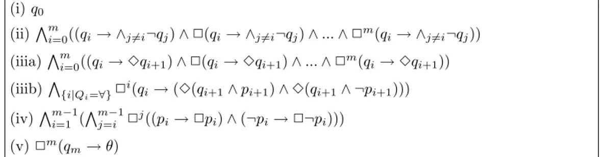
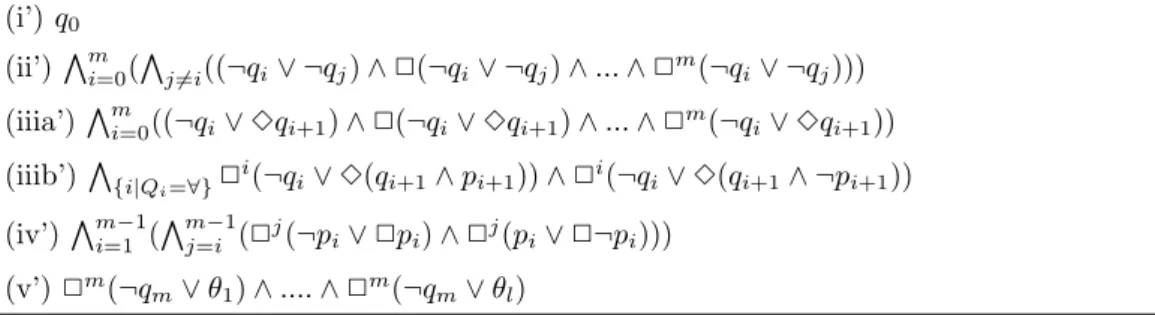
2.2 Encoding of QBF validity problem in Kn. . . 40
2.3 Embedding of Kn in first-order logic . . . 52
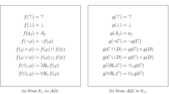
2.4 Mapping between Kn and ALC . . . 56
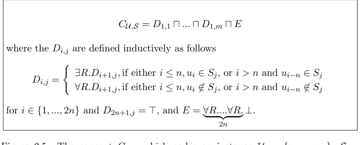
2.5 Encoding of exact cover problem in ALE . . . 59
3.1 Alternative encoding of QBF validity in Kn . . . 69
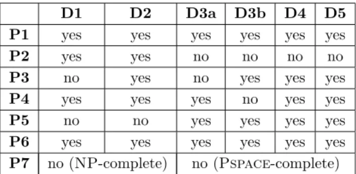
3.2 Properties of candidate definitions of literals, clauses, and terms. . . 76
2.1 Nnf . . . 32 2.2 Dnf . . . 33 2.3 Iter-Dnf . . . 33 2.4 Cnf . . . 38 2.5 Iter-Cnf . . . 38 2.6 Sat . . . 41 2.7 Entails . . . 44 2.8 LangInt . . . 48 4.1 GenPI . . . 91 4.2 Test3PI . . . 119 4.3 TestPI . . . 123 5.1 TestLangPI . . . 139 6.1 Π-Entail . . . 146 6.2 Π-LangInt . . . 163 6.3 Pinf . . . 180 xiii
Qu’est-ce que la génération de conséquences ?
La représentation des connaissances est une branche de l’intelligence artificielle qui étudie les différents formalismes permettant de répresenter des informations ainsi que les algorithmes qui permettent d’effectuer différentes tâches de raisonne-ments sur ces dernières. Une approche courante – celle que l’on adopte dans cette thèse – est d’utiliser des logiques formelles (la logique propositionnelle ou la logique du premier ordre, par exemple) comme langages de représentation des connais-sances. Dans cette approche, les informations sont représentées par des formules logiques, et le sens des formules est déterminé par la sémantique de la logique en question.
Lorsque la représentation des connaissances est basée sur une logique formelle, le principal problème lié au concept de raisonnement est celui de la déduction : étant données deux formules ϕ et ψ, l’objectif est de déterminer si ψ est une conséquence logique de ϕ, i.e. si ψ est vérifié chaque fois que ϕ l’est. Formellement :
est-ce que ϕ |= ψ ?
Nous verrons par la suite que dans certaines situations, une réponse simple de type “oui” ou “non” s’avère insuffisante. On s’intéressera alors à un problème plus général : générer les conséquences logiques d’une formule donnée. Formellement, ϕ étant donnée :
trouver les ψ tels que ϕ |= ψ
Cette tâche de raisonnement est communément appelée génération de conséquences [Mar00].
Quelles conséquences générer ?
Quand on parle de génération de conséquences, la première question qui se pose est de savoir quelles conséquences on souhaite générer. Nous ne pouvons clairement
2
pas produire toutes les conséquences logiques d’une formule, car toute formule pro-positionnelle a une infinité de conséquences. Et même en se restreignant à une seule conséquence par classe d’équivalence, nous produirions toujours beaucoup de conséquences redondantes ou non-pertinentes. Par exemple, si une formule a comme conséquence les formules ϕ et ψ, alors leur conjonction ϕ∧ψ est elle aussi une consé-quence de la formule. Or, il semble peu intéressant de générer ϕ ∧ ψ quand nous possédons déjà ϕ et ψ. De la même façon, si une formule a comme conséquence ϕ, alors toute formule de la forme ϕ ∨ ψ est également une conséquence, mais ces conséquences sont sans grand interêt. Il apparaît donc nécesssaire, avant toute ten-tative de générer les conséquences d’une formule, de définir le bon sous-ensemble de conséquences “pertinentes” à produire.
Comment peut-on formaliser la notion de “conséquence pertinente” ? En logique propositionnelle, la solution, due à Quine [Qui52, Qui55], est de considérer unique-ment les conséquences clausales les plus fortes de la formule1. Nous appelons ces clauses les impliqués premiers de la formule. En ne considérant que des clauses, qui ne contiennent pas de symboles de conjonction, nous éliminons les conséquences du type ϕ ∧ ψ, et en ne gardant que les conséquences clausales les plus fortes, nous éliminons les conséquences plus faibles de type ϕ ∨ ψ, où ϕ est une consé-quence. Comme chaque formule propositionnelle est équivalente à une conjonction de clauses, et chaque clause qui est impliquée par une formule ϕ est impliquée par un des impliqués premiers de ϕ, les impliqués premiers donnent une représentation complète et succincte de l’ensemble des conséquences logiques d’une formule. La génération de conséquences, à l’envers
Dans certaines situations, on s’intéresse non pas à l’ensemble des conséquences logiques d’une formule ϕ, mais plutôt à l’ensemble des “causes” de ϕ, c’est-à-dire l’ensemble des formules qui ont ϕ pour conséquence logique. Autrement dit, nous voulons faire de la génération de conséquences à l’envers. Formellement, étant don-née ϕ :
trouver les ψ tels que ψ |= ϕ
Comme pour la génération de conséquences « standard », il faut décider du type de formules que l’on souhaite produire : parmi toutes les formules ψ telles que ψ |= ϕ, quelles sont les formules intéressantes à générer ?
Comme nous faisons le contraire de la génération de conséquences, ce qu’il nous faut est l’opposé d’un impliqué premier ! Au lieu de considérer les clauses, nous
1
Nous rappelons qu’en logique propositionnelle un littéral est soit une variable propositionnelle soit la négation d’une variable propositionnelle, et qu’une clause est une disjonction de littéraux, e.g. a ∨ ¬b ∨ ¬c.
utilisons la notion duale de termes2, et au lieu de prendre les formules les plus fortes, nous prenons les plus faibles. La notion que nous obtenons ainsi est connue sous le nom d’implicant premier.
Comme on peut l’imaginer, les notions d’impliqué et d’implicant premier sont fortement liées. En effet, chacune de ces deux notions peut être définie en fonction de l’autre : les impliqués premiers de ϕ sont toutes les clauses dont la négation est équivalente à l’un des implicants premiers de ¬ϕ, et les implicants premiers de ϕ sont tous les termes dont la négation est équivalente à l’un des impliqués premiers de ¬ϕ. Grace à cette dualité, tous les résultats que nous obtiendrons sur les impliqués premiers pourront être transférés aux implicants premiers, et vice-versa.
Impliqués et implicants premiers : quelle utilité ?
Les impliqués et implicants premiers ont été utilisés dès les années 1950 dans le domaine de la conception de circuits électroniques. En effet, trouver un circuit de hauteur 2 représentant une formule ϕ donnée et possédant le moins de portes pos-sibles revient à trouver la représentation la plus compacte de ϕ comme disjonction d’implicants premiers ou comme conjonction d’impliqués premiers (voir Chapitre 4 de [BV04]). Les tableaux de Karnaugh, un classique des cours d’informatique de Licence, ne sont rien de plus qu’une méthode visuelle pour trouver une telle repré-sentation dans le cas de formules à 2 ou 3 variables. De même, le célèbre algorithme de minimisation de Quine-McCluskey [McC56] commence par calculer l’intégra-lité des implicants/impliqués premiers d’une formule, pour ensuite en extraire une couverture de coût minimal. Pour des formules à grand nombre de variables, des algorithmes heuristiques comme Espresso [BSVMH84] permettent de trouver une couverture de faible coût, sans toutefois en assurer l’optimalité.
A partir la fin des années 1980, les impliqués et implicants premiers ont fait leur apparition dans le domaine de l’intelligence artificielle. Depuis, ils ont été appliqués à de nombreuses problématiques, comme le raisonnement distribué [ACG+06], la ré-vision des croyances (cf. [Bit07], [Pag06], [BHQ08]), le raisonnement non-monotone (cf. [Prz89]), et l’étude de la pertinence (cf. [Lak95], [LLM03]). Mais les champs d’application les plus importants sont sans doute la compilation de connaissances et le raisonnement abductif. Dans la suite de cette section, nous étudions en détail le rôle de la génération de conséquences dans ces deux domaines.
2
4
Compilation de connaissances
Lorsque l’on base la représentation des connaissances sur la logique, une diffi-culté se présente immédiatement : les tâches de raisonnement ont une haute com-plextié algorithmique. En effet, même pour la logique propositionnelle, qui est parmi les moins expressives des logiques communément utilisées en représentation des connaissances, le problème de la déduction est co-NP-complet3. Il y a donc peu d’espoir de trouver des algorithmes de raisonnement qui terminent en un temps acceptable sur toutes les entrées.
La compilation de connaissances (cf. [CD97], [DM02]) est une technique générale pour faire face à la complexité élévée du raisonnement. Elle comporte deux phases : une phase préliminaire « hors ligne » dans laquelle la base de connaissances initiale (pour nous, une base est simplement une formule dans une logique donnée) est remplacée par une base équivalente dont la structure permettra, par la suite, un raisonnment efficace. S’en suit la phase « en ligne » dans laquelle nous effectuons des tâches de raisonnement sur la nouvelle base de connaissances. La phase préliminaire peut être difficile et coûteuse, mais l’idée est que ce coût initial sera compensé par les économies réalisées sur le raisonnement effectué pendant la deuxième phase.
Il existe un certain nombre de méthodes différentes pour compiler les formules de la logique propositionnelle, mais l’une des méthodes les plus connues est de représenter des formules par la conjonction de leurs impliqués premiers :
ϕ 7−→ π1∧ ... ∧ πn
Les formules propositionnelles sous cette forme ont de bonnes propriétés calcula-toires. En particulier, il est possible de tester en temps polynomial si une formule sous cette forme implique une formule en forme normale conjonctive (FNC). Afin de comprendre pourquoi, remarquons que ce dernier problème
π1∧ ... ∧ πn|= λ1∧ ... ∧ λm
se reduit à vérifier que pour chacune des clauses λi nous avons π1∧ ... ∧ πn|= λi
Si les formules πj étaient des clauses quelconques, ce dernier problème serait très difficile (co-NP-dur, pour être précis). Mais comme ce sont des impliqués premiers, nous pouvons profiter du fait que chaque clause impliquée par une formule doit l’être par l’un des impliqués premiers de la formule. En conséquence, nous avons simplement besoin de tester si l’une des formules πj implique λi :
pour chaque λi, tester s’il existe πj tel que πj |= λi
3
Enfin, nous remarquons que comme πj et λi sont des clauses, tester si πj |= λi est aussi simple que de vérifier que chaque littéral dans la clause πj est aussi dans λi :
les littéraux de πj sont-ils tous des littéraux de λi?
Nous avons décrit un algorithme simple et efficace pour tester si une formule repré-sentée par ses impliqués premiers implique une formule donnée en FNC.
Représenter les formules comme conjonction de leurs impliqués premiers permet également deux types de transformations importants : le conditonnement, où l’on assigne une valeur de vérité à l’une des variables propositionnelles d’une formule, et l’interpolation uniforme, où l’on projette une formule sur une signature donnée4. Pour comprendre pourquoi cette dernière tâche est facile (au sens algorithmique), remarquons que les impliqués premiers de la projection d’une formule sur une si-gnature sont précisément les impliqués premiers de la formule qui ne contiennent que des variables appartenant à la signature. Cela veut dire que si une formule est représentée comme conjonction de ses impliqués premiers, l’interpolation uniforme est aussi simple que d’enlever de la conjonction tous les impliqués premiers qui contiennent des variables n’appartenant pas à la signature.
Raisonnement abductif
L’abduction est un type de raisonnement dont le but est de produire des explica-tions possibles pour une observation donnée. Ce mode de raisonnement est central dans plusieurs domaines de l’intelligence artificielle, par exemple, le diagnostic, la planification, la compréhension du langage naturel, et la vision par ordinateur (se reporter à [EG95] pour les références). Du point du vue de la logique, un pro-blème d’abduction consiste en une observation (ce que nous voulons expliquer) et un ensemble de connaissances, tous les deux représentés par des formules logiques. L’objectif est de trouver une explication, c’est-à-dire une formule qui implique l’ob-servation (o) étant données les connaissances présupposées (t) :
trouver les e tels que t ∧ e |= o
Bien sûr, le nombre d’explications possibles peut être très important ; nous avons donc une nouvelle fois besoin d’un sous-ensemble d’explications “pertinentes”. Si nous réécrivons la tâche d’abduction comme ceci
trouver les e tels que e |= ¬t ∨ o
4
6
alors la réponse est évidente : nous devons utiliser les implicants premiers ! L’en-semble des explications pertinentes est alors simplement l’enL’en-semble des implicants premiers de ¬t ∨ o.
En réalité, un peu de prudence s’impose. Parmi les implicants premiers de ¬t ∨ o figurent les implicants premiers de ¬t, ce qui signifie que certaines des explications que nous générons peuvent être en contradiction avec la base de connaissances t. Ceci est clairement indésirable. Pour éliminer ces explications insatisfaisantes, nous exigeons de plus que les explications soient compatibles avec la base de connais-sances. Avec cette restriction supplémentaire, on obtient une version plus sophisti-quée du problème d’abduction :
trouver les e tels que t ∧ e |= o et t ∧ e 6|= ⊥ qui correspond à la tâche suivante
trouver les e tels que e |= ¬t ∨ o et e 6|= ¬t
Ce que nous cherchons vraiment est donc l’ensemble des implicants premiers de ¬t ∨ o qui n’impliquent pas ¬t. Cette variante de la notion d’implicant premier a été étudiée dans la littérature (cf. [Ino92], [del99] et discussion dans [Mar00]).
Une autre restriction couramment imposée à l’ensemble des explications est de demander que celles-ci soient construites à partir d’une signature donnée (cf. [EG95], [SL96]). Cela veut dire que nous souhaitons produire des implicants pre-miers qui ne contiennent que des variables propositionnelles de la signature. Cette variante de la notion d’implicant premier a été étudiée longuement dans la littéra-ture, et il existe plusieurs algorithmes de génération de conséquences qui peuvent produire des implicants premiers de ce type (cf. [Ino92], [del99], [SdV01], et discus-sion dans [Mar00]).
Au-delà de la logique classique
Pour de nombreuses applications en intelligence artificielle, la puissance expres-sive de la logique propositionnelle s’avère insuffisante. La logique du premier ordre offre une très grande expressivité, mais au prix de l’indécidabilité. Les logiques mo-dales et les logiques de description sont deux familles de logiques qui proposent un bon compromis entre expressivité et complexité, car elles sont en général plus expressives que la logique propositionnelle mais possèdent de meilleures propriétés calculatoires que la logique du premier ordre. Ceci explique la tendance croissante à utiliser ces logiques pour la représentation des connaissances.
Une limitation de la recherche actuelle sur la génération de conséquences est qu’elle se focalise quasi-exclusivement sur la logique propositionnelle et la logique du premier ordre. A notre connaissance, la génération de conséquences pour les logiques modales ou les logiques de description n’a jamais été étudiée. Cette lacune s’explique peut-être par le fait que la plupart des logiques modales et des logiques de description correspondent à des fragments de la logique du premier ordre. Il peut donc sembler inutile d’étudier la génération de conséquences pour ces logiques, car il est possible de traduire les formules de ces logiques en formules du premier ordre, puis d’appliquer les résultats et algorithmes déjà proposés pour la logique du premier ordre.
Le défaut de cet argument est que les impliqués et implicants premiers ne se com-portent pas aussi bien en logique du premier ordre qu’en logique propositionnelle. En effet, nous perdons en logique du premier ordre quelques propriétés clés comme la finitude (les formules peuvent avoir une infinité d’impliqués premiers distincts) et l’équivalence (une formule n’est pas nécéssairement équivalente à l’ensemble de ses impliqués premiers) [Mar91b, Mar91a]. Et comme par ailleurs les logiques modales ou de description possèdent souvent de bien meilleures propriétés calculatoires que la logique du premier ordre, on peut raisonnablement espérer obtenir de meilleurs résultats en faisant la génération de conséquences directement dans ces logiques, plutôt que de passer par la logique du premier ordre.
C’est pourquoi dans cette thèse nous proposons une étude de la génération de conséquences en logique modale, et plus précisement, dans la logique modale Kn. Nous avons choisi la logique Knpour deux raisons : d’une part il s’agit de la logique modale prototypique, et d’autre part elle possède de forts liens avec la logique de description ALC.
La question de savoir comment définir de façon appropriée les impliqués et implicants premiers dans la logique Knest clairement intéressante d’un point de vue théorique. Nous soutenons de plus qu’une solution satisfaisante serait prometteuse en termes d’applications. Passons brièvement en revue deux domaines d’application possibles.
Un premier domaine d’application potentiel est le raisonnement abductif dans Kn. Comme on l’a rappelé ci-dessus, l’une des questions fondamentales du raison-nement abductif est la sélection d’un sous-ensemble d’explications intéressantes. Cette question se pose avec encore plus de force pour les logiques comme Kn, pour lesquelles il peut y avoir une infinité de formules non-équivalentes (le nombre d’ex-plications distinctes pour un problème d’abduction peut donc être infini), rendant de facto impossible la génération de toutes les explications. Comme les implicants
8
premiers constituent la notion-clé permettant de caractériser les explications perti-nentes en logique propositionnelle, il semble qu’un bon point de départ de l’étude du raisonnement abductif dans Knserait de définir une notion d’impliqué premier pour cette logique. Nous allons dans ce qui suit proposer plusieurs définitions possibles, et comparer leurs propriétés respectives.
L’étude des impliqués premiers dans la logique Kn pourrait également se mon-trer utile pour le développement de méthodes de compilation pour cette logique. Actuellement, la quasi-totalité des travaux sur la compilation de connaissances se concentre sur la logique propositionnelle, bien que cette technique pourrait être étendue aux logiques modales et de description, pour lesquelles les tâches de rai-sonnement sont encore plus complexes qu’en logique propositionnelle. Ici encore, le rôle crucial de la notion d’impliqué premier en compilation de connaissances en logique propositionnelle suggère d’étendre cette notion à des logiques plus riches comme Kn.
Organisation de la thèse
Cette thèse constitue une exploration de la génération de conséquences dans la logique multi-modale Kn. Les principales questions que nous allons traiter sont les suivantes :
– Comment peut-on définir de façon appropriée les notions d’impliqué et impli-cant premier dans Kn? Quelles propriétés conservent ces notions par rapport à la logique propositionnelle ?
– Comment peut-on générer les impliqués premiers d’une formule de Kn? – Comment peut-on tester si une formule est un impliqué premier ? Quelle est
la complexité de cette tâche ?
– Combien d’impliqués premiers une formule peut-elle avoir ? Quelle est leur taille ?
– Comment utiliser les impliqués premiers pour compiler des formules dans Kn? Nous présentons maintenant un bref aperçu des différents chapitres qui com-posent cette thèse.
Chapitre 2. Ce chapitre constitue une introduction à la logique Kn. Les sujets abordés comprennent : la syntaxe et la sémantique de Kn, la terminologie et les notations, les propriétés de la conséquence logique, des transformations sur les for-mules dans Kn, les principales tâches de raisonnement et leur complexité, et les relations entre la logique Kn, la logique du premier ordre, et les logiques de
des-cription.
Chapitre 3. Dans ce chapitre, nous abordons la question de savoir comment les notions d’impliqué et d’implicant premier peuvent être définies de façon appropriée dans la logique Kn. Comme les impliqués et implicants premiers sont définis en logique propositionnelle au moyen des notions syntaxiques de clause et de terme, qui ne sont pas des notions standard dans Kn, nous commençons le chapitre par une étude de plusieurs définitions possibles de clauses et de termes dans Kn. Les différentes définitions sont évaluées à l’aune de leurs propriétés syntaxiques, sé-mantiques, et calculatoires. Nous commençons par définir un ensemble “idéal” de propriétés que l’on aimerait voire satisfaites par les clauses et les termes. Nous mon-trons qu’hélas, aucune de nos définitions de clause et de terme ne satisfait toutes ces propriétés (nous montrerons en effet qu’aucune définition possible ne les satisfait), mais deux de nos définitions s’en approchent raisonnablement. Dans la seconde par-tie du chapitre, nous examinons de nouveau les définitions proposées en fonction des notions d’impliqués et d’implicants premiers qu’elles induisent. Nous montrons alors qu’une seule de nos définitions candidates pour les notions de terme et clause induit des notions satisfaisantes d’impliqués et d’implicants premiers.
Chapitre 4. Ce chapitre étudie les propriétés calculatoires de la notion d’impliqué premier que nous avons séléctionnée dans le chapitre 3. Dans la première moitié du chapitre, nous proposons un algorithme correct et complet, GenPI, pour générer l’ensemble des impliqués premiers d’une formule de Kn. Notre algorithme fonc-tionne par décomposition : d’abord, nous écrivons la formule d’origine comme une disjonction de formules plus simples, puis nous calculons les impliqués premiers de ces dernières, et enfin nous utilisons ces impliqués premiers pour calculer les impliqués premiers de la formule d’origine.
Une analyse de la structure des impliqués premiers construits par notre algo-rithme nous permet de donner des bornes supérieures sur la taille et le nombre des impliqués premiers. Précisement, nous prouvons que chaque impliqué premier d’une formule ϕ est équivalent à une clause qui est au plus exponentiellement plus grande que ϕ et qu’une formule ne peut possèder dans le pire des cas qu’un nombre double-ment exponentiel d’impliqués premiers distincts. Nous démontrons que ces bornes sont optimales en donnant des bornes inférieures correspondantes, et nous prou-vons que ces bornes restent valables même pour des notions d’impliqués premiers beaucoup moins expressives.
La deuxième moitié du chapitre concerne la reconnaissance des impliqués pre-miers, qui est le problème de savoir si une clause est un impliqué premier d’une
10
formule donnée. Bien que cette question soit intéressante en soi, notre motivation principale est d’améliorer la complexité de notre algorithme de génération GenPI, qui utilise une méthode inefficace pour vérifier si une clause candidate est bien un impliqué premier. Nous proposons un algortihme correct et complet TestPI pour la reconnaissance des impliqués premiers, et nous montrons qu’il s’effectue en espace polynomial. Cela nous permet de prouver que le problème de reconnaissance est Pspace-complet, et donc de même complexité que la satisfiabilité et la déduction dans Kn.
Chapitre 5. Nous avons remarqué plus haut que certaines applications (comme l’abduction) peuvent nécessiter des variantes plus raffinées de la notion d’impliqué premier. C’est pourquoi dans le chapitre 5 nous examinons deux variantes de notre notion d’impliqué premier : les nouveaux impliqués premiers, qui nous permettent d’isoler les nouveaux faits que l’on peut déduire après l’ajout d’une information, et les impliqués premiers sur une signature, qui nous permettent de caractériser les conséquences d’une formule construites à partir d’une signature donnée. Nous étu-dions les propriétés de ces deux notions, en s’appuyant sur les résultats des chapitre précédents. Nous montrons en particulier que les impliqués premiers sur une signa-ture n’ont pas d’aussi bonnes propriétés calculatoires que les impliqués premiers standards.
Chapitre 6. Dans ce chapitre, nous nous interrogeons sur la possibilité d’utiliser notre notion d’impliqué premier afin de faire de la compilation de connaissances dans Kn, comme cela se fait en logique propositionnelle. En début de chapitre, nous expliquons pourquoi la façon la plus simple de définir une forme normale à partir de nos impliqués premiers n’est pas satisfaisante. Ceci nous amène à proposer notre propre définition, plus sophistiquée. Nous étudions les propriétés de notre forme normale, montrant en particulier qu’elle permet un test d’implication simple par comparaison syntaxique (qui est assez proche de le procédure décrite plus tôt dans le chapitre pour la logique propositionnelle).
Nous montrons aussi que l’interpolation uniforme est facile (au sens calcula-toire) pour les formules de Kn mises sous forme normale. Nous étudions ensuite la complexité de la mise sous forme normale des formules de Kn, et proposons un algorithme pour effectuer cette tâche. Nous concluons le chapitre par une compa-raison de notre forme normale aux autres formes normales pour Kn proposées dans la littérature.
Chapitre 7. Ce chapitre résume les principales contributions de la thèse, et pro-pose quelques pistes intéressantes pour des recherches futures.
1
Introduction
What is consequence finding?
Knowledge representation is a subfield of artificial intelligence which is con-cerned with the study of formalisms for representing different kinds of information and the development of procedures for performing reasoning on these representa-tions. Many knowledge representation formalisms exist, but one popular approach, and the one we adopt in this thesis, is to utilize formal logics (propositional logic, first-order logic, etc.) as knowledge representation languages. According to this approach, information is represented using logical formulae, and the meaning of formulae is determined by the semantics of the logic in question.
The major reasoning task in logic-based knowledge representation is that of deduction: given two formulae, let’s call them ϕ and ψ, our job is to determine whether ψ is a logical consequence of ϕ, i.e. whether the truth of ϕ guarantees the truth of ψ. Symbolically,
does ϕ |= ψ?
As we shall see later in the section, there are circumstances in which such a simple “yes” or “no” answer proves insufficient. Instead, what we are interested in is the more general problem of generating logical consequences of a particular formula:
find ψ such that ϕ |= ψ
This reasoning task is commonly known as consequence finding [Mar00]. 13
14
But which consequences should we generate?
One of the first questions that presents itself when we talk about consequence finding is which consequences do we generate? We obviously cannot generate all of the consequences of a formula, because even the simplest propositional formula has infinitely many consequences. Even if we restrict ourselves to one consequence per equivalence class, we still produce a lot of clearly irrelevant or redundant conse-quences. Indeed, if a formula has both ϕ and ψ as consequences, then the formula ϕ∧ ψ is also a consequence, but it seems entirely superfluous once we have ϕ and ψ. Likewise, if a formula has a consequence ϕ, then every formula of the form ϕ ∨ ψ is also a consequence, but these consequences don’t seem to hold much interest. What we need is a way of focusing in on a relevant subset of consequences.
How can we formalize the notion of a relevant or interesting consequence? In propositional logic, the solution, due to Quine [Qui52, Qui55], is to consider only the logically strongest clauses1 which are consequences of the formula. We call these clauses the formula’s prime implicates. By focusing on clauses, which do not contain any conjunction symbols, we avoid redundant consequences of the type ϕ∧ ψ, and by only considering the logically strongest clausal consequences, we eliminate weaker, irrelevant consequences of the type ϕ ∨ ψ. As every propositional formula can be rewritten as a conjunction of clauses, and every clausal consequence of a formula is entailed by some prime implicate of the formula, prime implicates provide a complete yet compact representation of a formula’s consequences.
Consequence finding, in reverse
In some circumstances, we may be interested not in the logical consequences of a given formula, but rather the formulae which have this formula as a consequence. Basically, we want to do consequence finding in reverse:
find ψ such that ψ |= ϕ
Just as for standard consequence finding, a key issue is selecting the right set of formulae to generate: of the many ψ which satisfy ψ |= ϕ, which ones should we choose?
Well, since we are doing the opposite of consequence finding, what we need is the opposite of a prime implicate! Instead of clauses, we can use the dual notion of terms2, and instead of taking the logically strongest formulae, we take the logically weakest. The resulting notion is known as a prime implicant.
1. We recall that in propositional logic a literal is a propositional variable or the negation of a propositional variable, and a clause is a disjunction of literals, e.g. a ∨ ¬b ∨ ¬c.
As one might expect, prime implicates and prime implicants are very closely related. Indeed, each of these notions can be defined in terms of the other: the prime implicates of ϕ are just the clauses which are equivalent to the negation of a prime implicant of ¬ϕ, and the prime implicants of ϕ are precisely those terms whose negations are equivalent to prime implicates of ¬ϕ. This means that all of the results concerning prime implicates can be transferred to prime implicants, and vice-versa.
Prime implicates and prime implicants: what are they good for?
Prime implicates and prime implicants have been used since the fifties in the field of digital circuit synthesis: the design of minimal-cost two-level circuits comes down to finding the shortest way of representing a propositional formula as ei-ther a disjunction of a subset of its prime implicants or a conjunction of some of its prime implicates (cf. Chapter 4 of [BV04]). Karnaugh maps, a staple of un-dergraduate computer science courses, are really nothing more than a visual tool for isolating covering sets of prime implicants/implicates, and the famous Quine-McCluskey minimization algorithm [McC56] works by first generating the entire set of prime implicants/implicates, then computing the covering subsets with min-imal cost. For circuits with large numbers of variables, heuristic methods, like Espresso [BSVMH84], allow one to produce good but not necessarily optimal prime implicate/implicant covers without the computation of the entire set of prime im-plicates/implicants.
Starting from the late eighties, prime implicates and prime implicants began to appear in the artificial intelligence literature. Since then, these notions have been utilized for a number of different AI problems, such as distributed reasoning [ACG+06], belief revision (cf. [Bit07], [Pag06], [BHQ08]), non-monotonic reasoning (cf. [Prz89]), and characterizations of relevance (cf. [Lak95], [LLM03]). Probably the most important domains of application, however, are knowledge compilation and abductive reasoning. In the remainder of this section, we present a detailed look at the role of consequence finding in these two areas.
Knowledge compilation
One major obstacle for logic-based knowledge representation is the high com-putational complexity of reasoning. Indeed, even for propositional logic, which is among the least expressive knowledge representation languages, the basic reason-ing task of deduction is co-NP-complete3. This means that there is little hope of
16
finding reasoning algorithms which terminate in a reasonable amount of time on all inputs.
Knowledge compilation (cf. [CD97], [DM02]) is a general technique for coping with the intractability of reasoning. It consists of two phases: a preliminary off-line phase in which we replace the original knowledge base (for us, this is just a formula in some logic) by an equivalent knowledge base which admits efficient reasoning, followed by a second online phase in which we perform reasoning tasks on the compiled knowledge base. The off-line phase may prove difficult and costly, but the idea is that this initial cost will be offset by the computational savings on the reasoning done during the online phase.
There exist a number of different methods for compiling propositional formulae, but one of the better-known approaches is to use prime implicate normal form4, in which a formula is represented as the conjunction of its prime implicates:
ϕ 7−→ π1∧ ... ∧ πn
Propositional formulae in prime implicate normal form have many nice computa-tional properties. In particular, it is possible to test in polynomial time whether a formula in prime implicate normal form entails a formula in conjunctive normal form (CNF). To see why, we first remark that this problem
π1∧ ... ∧ πn|= λ1∧ ... ∧ λm
can be reduced to testing whether for each of the clauses λi we have π1∧ ... ∧ πn|= λi
Now if the conjuncts πj were arbitrary clauses, then the latter problem would be very difficult (co-NP-hard, to be precise). But because we are dealing with prime implicates, we can take advantage of the fact that every clause implied by a formula must be implied by one of the formula’s prime implicates. This means that we just need to find a single conjunct πj which implies λi:
for each λi, check whether there is some πj such that πj |= λi
Finally, we remark that since the πjand λiare all clauses, deciding whether πj |= λi is easy since we just need to test whether each of the literals appearing in πj also appears in λi:
is each disjunct of πj also a disjunct of λi?
4. Prime implicant normal form also exists, but is a bit less common. It offers many of the same advantages as prime implicate normal form, the exception being that the uniform interpolation transformation is not tractable [DM02].
We have thus outlined a simple and efficient procedure for determining whether a formula in prime implicate normal form implies a formula in CNF. Notice that this procedure can also be used to decide entailment or equivalence between two formulae in prime implicate normal form in polynomial time.
Prime implicate normal form also supports two important transformations: con-ditioning, in which we assign a truth value to one of a formula’s propositional variables, and uniform interpolation (or forgetting), in which we approximate a formula over a given signature5. To see why the latter task is tractable, we re-mark that the prime implicates of the approximation of a formula over a signature are precisely those prime implicates of the original formula which do not contain any propositional variables outside the signature. This means that for formulae in prime implicate normal form, uniform interpolation is as simple as removing those conjuncts which contain one of the unwanted propositional variables.
Abductive reasoning
Abduction is a form of reasoning that is used to generate explanations for obser-vations. It has been applied to a number of different areas in artificial intelligence, e.g. diagnosis, planning, natural language understanding, and computer vision (re-fer to [EG95] for re(re-ferences). In logic-based approaches to abduction, an abduction problem typically consists of an observation (what we want to explain) and some background knowledge, both of which are represented by logical formulae. The objective is to find an explanation, that is, a formula which logically entails the observation (o) when taken together with the background theory (t):
find e such that t ∧ e |= o
Of course, the number of possible explanations might be very large, so we need a way of characterizing the interesting explanations. If we rewrite the abduction task in terms of reverse consequence finding as follows
find e such that e |= ¬t ∨ o
then the answer becomes obvious: we should use prime implicants! Thus, we can define the set of interesting explanations to be the prime implicants of ¬t ∨ o.
Well, actually we need to be a bit more careful. Among the prime implicants of ¬t∨o are the prime implicants of ¬t, which means that some of the explanations we generate may be in contradiction with the background knowledge. This is clearly undesirable, so in order to eliminate these unsatisfactory explanations, we generally
18
place an additional requirement on explanations, namely that they be consistent with the background theory. This yields the following more sophisticated abduction problem:
find e such that t ∧ e |= o and t ∧ e 6|= ⊥
which corresponds, in consequence finding terms, to the following task find e such that e |= ¬t ∨ o and e 6|= ¬t
So what we are after are those prime implicants of ¬t ∨ o which do not imply ¬t. This variant on the basic notion of prime implicant has been investigated in the consequence finding literature (cf. [Ino92], [del99] and discussion in [Mar00]).
Another common restriction on explanations is to require that they are built from a specified signature (cf. [EG95], [SL96]). In consequence-finding terms, this means that we want to look for prime implicants which only contain propositional variables belonging to the given signature. This more refined notion of prime impli-cant has been studied extensively in the literature, and many consequence-finding algorithms exist for producing prime implicants of this type (cf. [Ino92], [del99], [SdV01], and discussion in [Mar00]).
Going beyond classical logic
For many applications in artificial intelligence, the expressive power of propo-sitional logic proves insufficient. First-order logic provides a much greater level of expressivity, but at the price of undecidability. Modal and description logics are two families of logics which offer an interesting trade-off between expressivity and complexity, as they are generally more expressive than propositional logic yet are better-behaved computationally than first-order logic. This explains the growing trend towards using such languages for knowledge representation.
One limitation of current research in consequence finding is that it is focused almost exclusively on classical propositional and first-order logic (with an emphasis on the former). To our knowledge, there has not been any research concerning consequence finding for modal and description logics. Perhaps one explanation for this is that most modal and description logics correspond to fragments of first-order logic. Thus, one might argue that it is unnecessary to study consequence finding for these logics, since we can just map our formulae to first-order logic and do consequence finding there.
The problem with this argument is that prime implicates and prime implicants do not behave as nicely in first-order logic as in propositional logic. Indeed, we lose some key properties like finiteness (first-order logic formulae can have infinitely
many distinct prime implicates) and equivalence (a first-order formula is not nec-essarily equivalent to its set of prime implicates) [Mar91b, Mar91a]. Given that modal and description logics have better computational properties than first-order logic, there is reason to believe that we might have better luck doing consequence finding directly in these logics, without passing by first-order logic.
This is why in this thesis we propose to study consequence finding in modal logic, and more specifically, in the modal logic Kn. We decided to study Knbecause it is the prototypical modal logic, and also because of its close relationship with the well-known description logic ALC. Indeed, while the results in this thesis are presented in terms of Kn formulae, all of our results hold equally well for ALC concept expressions.
The question of how the notions of prime implicates and prime implicants can be suitably defined for the logic Kn is clearly of interest from a theoretical point of view. We argue, however, that this question is also practically relevant. To support this claim, we briefly discuss two application areas in which the study of prime implicates and prime implicants in Kn might prove useful.
One potential domain of application is abductive reasoning in Kn. As noted above, one of the key foundational issues in abductive reasoning is the selection of an interesting subset of explanations. This issue is especially crucial for logics like Kn which allow for an infinite number of non-equivalent formulae, since this means that the number of non-equivalent explanations for an abduction problem is not just large but in fact infinite, making it simply impossible to enumerate the entire set of explanations. As prime implicants are a widely-accepted means of characterizing relevant explanations in propositional logic, a reasonable starting point for research into abductive reasoning in the logic Kn is the study of different possible definitions of prime implicant in Kn and their properties.
The investigation of prime implicates in Knis also relevant to the development of knowledge compilation procedures for Kn. Currently, most work on knowledge com-pilation is restricted to propositional logic, even though this technique could prove highly relevant for modal and description logics, which generally suffer from an even higher computational complexity than propositional logic. As prime implicates are one of the better-known mechanisms for compiling formulae in propositional logic, it certainly makes sense to investigate whether this approach to knowledge compi-lation can be fruitfully extended to logics like Kn.
20
Organization of this thesis
This thesis constitutes an exploration of consequence finding in the basic modal logic Kn. The main questions that we will be addressing are the following:
• How can prime implicates and prime implicants be appropriately defined in the logic Kn? What are the properties of the resulting notions?
• How can one generate the prime implicates of formulae in Kn?
• How can one test whether a formula is indeed a prime implicate? What is the complexity of this task?
• How many prime implicates can a Kn-formula have? How large can these prime implicates be?
• How can prime implicates be used for compiling Kn-formulae? We now present a brief overview of the different chapters of this thesis.
Chapter 2. This chapter provides the necessary background material for later chapters. Topics covered include: syntax and semantics of Kn, terminology and no-tation, properties of logical consequence, transformations on Knformulae, principal reasoning tasks and their complexities, and the relationship of Knto first-order logic and description logics.
Chapter 3. In this chapter, we address the question of how the notions of prime implicates and prime implicants can be appropriately lifted from propositional logic to Kn. As prime implicates and prime implicants are defined in terms of the notions of clauses and terms, which are not standard notions in Kn, we begin the chapter by considering a number of potential definitions of clauses and terms for Kn. The different definitions are evaluated with respect to a set of syntactic, semantic, and complexity-theoretic properties characteristic of the propositional definition. None of the definitions satisfies all of these properties (indeed we show this to be impos-sible), but two of the definitions come reasonably close. In the second half of the chapter, we take a second look at the candidate definitions, this time evaluating them with respect to the properties of the notions of prime implicates and prime implicants that they induce. We show that only one of the candidate definitions yields a satisfactory notion of prime implicates and prime implicants.
Chapter 4. This chapter investigates the computational properties of our selected definition of prime implicate. In the first half of the chapter, we propose a sound and complete algorithm GenPI for generating prime implicates. Our algorithm adopts a decomposition-style approach: first, we rewrite the original formula as
a disjunction of simpler formulae, then we compute the prime implicates of these simpler formulae, and finally, we use the prime implicates of the simpler formulae to help us compute the prime implicates of the original formula.
An analysis of the structure of the prime implicates constructed by our algo-rithm allows us to place upper bounds on the size and number of prime implicates. Specifically, we demonstrate that every prime implicate of a formula is equivalent to a clause which is no more than single-exponentially larger than the formula, and that a formula can possess no more than double-exponentially many prime implicates modulo equivalence. We prove these upper bounds optimal by providing matching lower bounds, and then we go further and show that the lower bounds hold even for much less expressive notions of prime implicates.
The focus of the second half of the chapter is on prime implicate recognition, which is the problem of deciding whether a given clause is a prime implicate of a formula. While this problem is interesting in and of itself, an additional motivation for studying this task is to improve our generation algorithm GenPI, which utilizes a very inefficient method for verifying whether a candidate clause is indeed a prime implicate. We propose a sound and complete procedure TestPI for recognizing prime implicates, and we show that it runs in polynomial space. This allows us to prove that the prime implicate recognition task is Pspace-complete, and hence of the same complexity as standard reasoning tasks in Kn.
Chapter 5. We saw earlier in the chapter that some applications (like abduc-tion) can require more refined notions of prime implicates/implicants. This is why in Chapter 5 we study two variants on our notion of prime implicate: new prime implicates, which allow us to isolate the novel facts which can be derived upon arrival of new information, and signature-bounded prime implicates, which allow one to characterize the consequences of a formula which are built from a given signature. We investigate the properties of these notions, leveraging results from earlier chapters. We show in particular that signature-bounded prime implicates are less well-behaved computationally than regular prime implicates.
Chapter 6. This chapter is concerned with the application of our notion of prime implicate to the area of knowledge compilation. We begin the chapter by showing why the obvious definition of prime implicate normal form in Kn is unsatisfactory, before proposing our own more sophisticated definition. We investigate the prop-erties of our normal form, showing in particular that entailment between formulae in prime implicate normal form can be carried out in quadratic time using a simple structural comparison algorithm (which is quite similar to the procedure outlined
22
earlier in the chapter for propositional logic). We also show that uniform inter-polation is tractable for formulae in our normal form. Later in the chapter, we propose an algorithm for putting formulae into prime implicate normal form, and we investigate the spatial complexity of this transformation, showing there to be an at most double-exponential blowup in formula size. We conclude the chapter with a comparison of prime implicate normal form to existing normal forms for Kn formulae.
Chapter 7. In this chapter, we summarize the main contributions of the thesis and indicate some interesting avenues of future research.
Appendix A. We provide in this appendix a brief review of computational com-plexity theory, in which we recall the definitions of the different comcom-plexity classes appearing in this thesis.
Relevant publications
Some of the results presented in this thesis have been previously published: • A complete version of Chapters 3 and 4 can be found in the journal paper
[Bie09]. Many of the results of Chapter 3 and some results from Chapter 4 first appeared in an earlier conference paper [Bie07b] (but with some errors). • Some parts of Chapter 5 were presented in the workshop paper [Bie07a]. • Many of the results in Chapter 6, rephrased in terms of the description logic
ALC, were published in [Bie08b] (and were also presented in [Bie08c]). Two related publications which were obtained during the author’s doctoral studies but are not presented in this thesis are:
• [BHQ08], which introduces a prime-implicate based revision procedure • [Bie08a], which presents complexity results for abductive reasoning in the EL
2
The Modal Logic
K
n
In this chapter, we introduce the basics of the modal logic Kn1. We begin by recalling the syntax and semantics of the logic Kn and introducing some key notation and terminology. Next, we highlight some properties of logical consequence in Kn which will prove useful to us in later chapters. After that, we introduce some basic transformations and reasoning tasks in Kn and study their properties. Finally, at the end of the chapter, we discuss the relationship of the modal logic Kn with first-order logic and with description logics.
Several of the results presented in this chapter have appeared previously in the literature, but we have chosen to include proofs of these results in order to make this thesis as self-contained as possible.
2.1
Syntax
Formulae in Knare built up from a set of propositional variables V, the standard logical connectives (¬, ∧, and ∨), and the modal operators 2i and 3i (for 1 ≤ i ≤ n). For convenience, we will also include the special zero-ary connectives ⊤ and ⊥ to represent the tautology and contradiction, and we will often treat ∧ and ∨ as multiple-arity connectives. In the special case where n = 1, we will write K instead of K1, and we will use 2 and 3 in place of 21 and 31.
Where convenient, we will use ϕ → ψ as an abbreviation for ¬ϕ ∨ ψ. We adopt the shorthand 2kiϕ(resp. 3kiϕ) to refer to the formula consisting of ϕ preceded by kcopies of 2i (resp. 3i), with the convention that 20iϕ= 30iϕ= ϕ.
1. Refer to [BdV01], [Che80], or [BvW06] for good introductions to modal logic.
24 2.1. Syntax
We will use var(ϕ) to refer to the set of propositional variables appearing in a formula ϕ. A signature for Kn is defined to be a subset of V ∪ {1, 2, ..., n}. For example, if V = {a, b, c} and n = 3, then both {1, 3, a} and {a, b, c} would be valid signatures. The signature of a formula ϕ, written sig(ϕ), is defined to be the union of var(ϕ) and the set of numbers j such that 2j or 3j appears in ϕ. For example, we have sig(2132(a ∨ c)) = {1, 2, a, c}.
The (modal) depth of a formula ϕ, written δ(ϕ), is defined as the maximal number of nested modal operators appearing in ϕ, e.g. δ(3(a ∧ 2a) ∨ a) = 2. We define the length (or size) of a formula ϕ, written |ϕ|, to be the number of occurrences of propositional variables, logical connectives, and modal operators in ϕ. So for example, we would have |(a ∧ ¬b)| = 4 and |31(a ∨ b) ∧ 22a| = 7.
The set of subformulae of a formula ϕ, denoted Sub(ϕ), is defined recursively as follows:
Sub(⊤) = {⊤} Sub(⊥) = {⊥}
Sub(a) = {a}(for a ∈ V) Sub(¬ψ) = {¬ψ} ∪ Sub(ψ)
Sub(ψ1∧ ψ2) = {ψ1∧ ψ2} ∪ Sub(ψ1) ∪ Sub(ψ2) Sub(2iψ) = {2iψ} ∪ Sub(ψ) Sub(ψ1∨ ψ2) = {ψ1∨ ψ2} ∪ Sub(ψ1) ∪ Sub(ψ2) Sub(3iψ) = {3iψ} ∪ Sub(ψ) For example, the subformulae of ¬(a ∨ 22(b ∧ 31⊤)) are: ¬(a ∨ 22(b ∧ 31⊤)), a∨ 22(b ∧ 31⊤), a, 22(b ∧ 31⊤), b ∧ 31⊤, b, 31⊤, and ⊤. It is easily shown by induction that the cardinality of Sub(ϕ) can never exceed |ϕ|.
An occurrence of a subformula σ of a formula ϕ is said to be in the scope of a modal operator q just in the case that there is a subformula qχ of ϕ such that χ contains the occurrence of σ. For instance, the first occurrence of the subformula a in (2132a) ∨ ¬a is in the scope of the modal operators 21 and 32, but the second occurrence of a is outside the scope of any modal operators.
We will call a formula of the form 2iϕ (resp. 3iϕ) a 2-formula (resp. 3-formula). We will say that a formula is basic if it is either a propositional literal or a 2- or 3-formula. A formula will be called disjunctive if it is a disjunction of basic formulae. A formula is said to be conjunctive if it is a conjunction of basic formulae.
We introduce some notation in order to refer to different components of dis-junctive and condis-junctive formulae. If ϕ is a disdis-junctive (resp. condis-junctive) for-mula, then P rop(ϕ) is defined to be the set of propositional literals which are disjuncts (resp. conjuncts) of ϕ. If ϕ is a disjunctive (resp. conjunctive) formula, then Boxi(ϕ) is defined to be the set of formulae ψ such that 2iψ is a disjunct (resp. conjunct) of ϕ. Similarly, Diami(ϕ) is defined as the set of formulae ψ such that 3iψ is a disjunct (resp. conjunct) of ϕ. For example, for the disjunc-tive formula ϕ = ¬a ∨ ¬b ∨ 21c∨ 2132⊤ ∨ 31⊤, we have P rop(ϕ) = {¬a, ¬b},
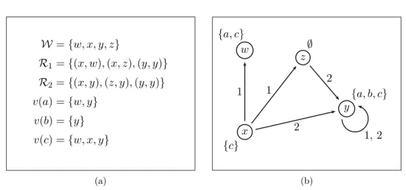
W = {w, x, y, z}
R1= {(x, w), (x, z), (y, y)} R2= {(x, y), (z, y), (y, y)} v(a) = {w, y} v(b) = {y} v(c) = {w, x, y} (a) w {a, c} x {c} z ∅ y {a, b, c} 1 1 2 2 1, 2 (b)
Figure 2.1: An example model and its graphical representation.
Box1(ϕ) = {c, 32⊤}, Box2(ϕ) = Diam2(ϕ) = ∅, and Diam1(ϕ) = {⊤}. For the conjunctive formula ψ = c∧21⊥∧22a∧32(a∨21b)∧32c, we have P rop(ψ) = {c}, Box1(ψ) = {⊥}, Box2(ψ) = {a}, Diam1(ψ) = ∅, and Diam2(ψ) = {a ∨ 21b, c}.
A Kn-formula is said to be in negation normal form (NNF) just in the case that it does not contain → and every negation symbol appears directly in front of propo-sitional variables. Every formula in Kn can be transformed in linear time into an equivalent formula in NNF of the same modal depth via a straightforward applica-tion of the standard logical equivalences. More details on the NNF transformaapplica-tion can be found in Section 2.4.
2.2
Semantics
A model (or interpretation) for Knis a tuple M = hW, {Ri}ni=1, vi, where W is a non-empty set of possible worlds, each Ri⊆ W ×W is a binary relation over worlds, and v : V → 2W defines for each propositional variable the set of worlds in which the variable holds. Models can be seen as labelled directed graphs, in which the vertices correspond to the elements of W, the directed edges represent the binary relations, and the vertices are labelled by the set of propositional variables which hold in the corresponding possible world. In Figure 2.1, we give an example of a model and its corresponding graphical representation.
Satisfaction of a formula ϕ in a model M at the world w (written M, w |= ϕ) is defined inductively as follows:
• M, w |= ⊤ • M, w 6|= ⊥
26 2.3. Logical Consequence
• M, w |= a if and only if w ∈ v(a) • M, w |= ¬ϕ if and only if M, w 6|= ϕ
• M, w |= ϕ ∧ ψ if and only if M, w |= ϕ and M, w |= ψ • M, w |= ϕ ∨ ψ if and only if M, w |= ϕ or M, w |= ψ
• M, w |= 2iϕif and only if M, w′ |= ϕ for every w′ such that (w, w′) ∈ Ri • M, w |= 3iϕif and only if M, w′ |= ϕ for some w′ such that (w, w′) ∈ Ri If we think of models as labelled directed graphs, then determining the satisfaction of a formula 2iϕ at vertex w consists in evaluating ϕ at all of the vertices which can be reached from w via an i-labelled edge; 2iϕ is satisfied at w just in the case that ϕ holds in each of these successor vertices. Similarly, in order to decide whether a formula 3iϕholds at a vertex w, we consider each of the i-successors of w in the graph and check whether at least one of these vertices satisfies ϕ.
Example 2.2.1.
Let M be the model defined in Figure 2.1. We have: • M, w |= a, since w ∈ v(a)
• M, w |= 21⊥, since there is no world u such that (w, u) ∈ R1 • M, w |= a ∧ 21⊥, since both M, w |= a and M, w |= 21⊥ • M, z |= ¬a, since M, z 6|= a
• M, x |= 31¬a, since (x, z) ∈ R1 and M, z |= ¬a
• M, x |= 2121⊥, since w and z are the only 1-successors of x, and both M, w|= 21⊥ and M, z |= 21⊥
• M, x |= 22(a ∧ b ∧ c), since the only 2-successor of x is y and M, y |= a ∧ b ∧ c A formula ϕ is said to be a tautology, written |= ϕ, if M, w |= ϕ for every model M and world w. A formula ϕ is satisfiable if there is some model M and some world w such that M, w |= ϕ. If there is no M and w for which M, w |= ϕ, then ϕ is called unsatisfiable, and we write ϕ |= ⊥.
2.3
Logical Consequence
In modal logic, there are two different ways of defining logical consequence (cf. [van83] for discussion):
• a formula ψ is a global consequence of ϕ if whenever M, w |= ϕ for every world w of a model M, then M, w |= ψ for every world w of M
• a formula ψ is a local consequence of ϕ if M, w |= ϕ implies M, w |= ψ for every model M and world w
In this thesis, we will be focusing on local consequence, firstly because this is the notion of consequence most often used in the modal logic literature, and secondly
because the local consequence relation is better-behaved than the global conse-quence relation in some important respects. In particular, the deduction theorem, familiar from classical logic, holds only with respect to the local consequence rela-tion. In what follows, we will take ϕ |= ψ to mean that ψ is a local consequence of ϕ, and we will say that ϕ (logically) entails ψ. Two formulae ϕ and ψ will be called equivalent, written ϕ ≡ ψ, if both ϕ |= ψ and ψ |= ϕ. A formula ϕ is said to be logically stronger than ψ if ϕ |= ψ and ψ 6|= ϕ.
In the remainder of this section, we highlight some basic properties of logical consequence in Kn, some well-known and some less so, which will play an important role in the proofs of our results.
Theorem 2.3.1.
Let γ be a propositional formula, let ψ, χ, ψi, χi, ψi,j, χi,j be formulae in Kn, and let k be an integer between 1 and n. Then
1. ψ |= χ ⇔ |= ¬ψ ∨ χ ⇔ ψ ∧ ¬χ |= ⊥ 2. 3kψ≡ ¬2k¬ψ
3. ψ |= χ ⇔ 3kψ|= 3kχ⇔ 2kψ|= 2kχ
4. 2k(ψ1∧ ψ2∧ ... ∧ ψm) ≡ 2kψ1∧ 2kψ2∧ ... ∧ 2kψm 5. 3k(ψ1∨ ψ2∨ ... ∨ ψm) ≡ 3kψ1∨ 3kψ2∨ ... ∨ 3kψm
6. γ ∧Vni=1(3iψi,1∧ ... ∧ 3iψi,li∧ 2iχi,1∧ ... ∧ 2iχi,mi) |= ⊥
⇔ γ |= ⊥ or ψi,j∧ χi,1∧ ... ∧ χi,mi |= ⊥ for some 1 ≤ i ≤ n and 1 ≤ j ≤ li
7. |= γ ∨Wni=1(3iψi,1∨ ... ∨ 3iψi,li∨ 2iχi,1∨ ... ∨ 2iχi,mi)
⇔ |= γ or |= ψi,1∨ ... ∨ ψi,li ∨ χi,j for some 1 ≤ i ≤ n and 1 ≤ j ≤ mi
8. 2kχ|= 2kχ1∨ ... ∨ 2kχm ⇔ χ |= χi for some 1 ≤ i ≤ m 9. 3kψ1∨ ... ∨ 3kψl∨ 2kχ1∨ ... ∨ 2kχm
≡ 3kψ1∨ ... ∨ 3kψl∨ 2k(χ1∨ ψ1∨ ... ∨ ψl) ∨ ... ∨ 2k(χm∨ ψ1∨ ... ∨ ψl) Proof. The first statement is a well-known property of local consequence, but we prove it here for completeness:
ψ|= χ ⇔ M, w |= ψ implies M, w |= χ for all M, w ⇔ M, w 6|= ψ or M, w |= χ for all M, w ⇔ M, w |= ¬ψ or M, w |= χ for all M, w ⇔ |= ¬ψ ∨ χ
⇔ M, w 6|= ψ ∧ ¬χ for all M, w ⇔ ψ ∧ ¬χ |= ⊥
28 2.3. Logical Consequence
The second statement is also standard, and can be simply proved as follows: M, w|= 3kψ ⇔ there is some v such that (w, v) ∈ Rk and M, v |= ψ
⇔ there is some v such that (w, v) ∈ Rk and M, v 6|= ¬ψ ⇔ M, w 6|= 2k¬ψ
⇔ M, w |= ¬2k¬ψ
For the third statement, if ψ 6|= χ, then there is some M, w such that M, w |= ψ∧ ¬χ. Create a new model M′ from M by adding a new world w′ and placing a single k-arc from w′ to w. Then M′, w′ |= 3kψ∧ 2k¬χ, which means that 3kψ∧ 2k¬χ is satisfiable and hence 3kψ 6|= 3kχ (using statements 1 and 2). For the other direction, suppose 3kψ 6|= 3kχ. Then there exists M, w such that M, w |= 3kψ∧ ¬3kχ ≡ 3kψ∧ 2k¬χ. But this means that there is some w′ for which ψ ∧ ¬χ, hence ψ 6|= χ. To complete the proof, we use the following chain of equivalences: 2kψ|= 2kχ ⇔ ¬2kχ|= ¬2kψ ⇔ 3k¬χ |= 3k¬ψ ⇔ ¬χ |= ¬ψ ⇔ ψ|= χ.
For statement 4, we have M, w |= 2k(ψ1∧ ψ2∧ ... ∧ ψm) if and only if M, w′ |= ψ1∧ ψ2∧ ... ∧ ψm for every w′ with wRkw′ if and only if M, w′ |= ψi for every w′ with wRkw′ and 1 ≤ i ≤ m if and only if M, w |= 2kψi for every 1 ≤ i ≤ m if and only if M, w |= 2kψ1∧ 2kψ2∧ ... ∧ 2kψm.
Statement 5 is shown as follows: M, w |= 3k(ψ1 ∨ ψ2 ∨ ... ∨ ψm) if and only if M, w′ |= ψ1∨ ψ2∨ ... ∨ ψm for some w′ with wRkw′ if and only if M, w′ |= ψi for some 1 ≤ i ≤ m and w′ with wR
kw′ if and only if M, w |= 3kψi for some 1 ≤ i ≤ m if and only if M, w |= 3kψ1∨ 3kψ2∨ ... ∨ 3kψm.
For 6, suppose γ ∧Vni=1(3iψi,1∧ ... ∧ 3iψi,li∧ 2iχi,1∧ ... ∧ 2iχi,mi) 6|= ⊥. Then
there exist M, w such that M, w |= γ ∧Vni=1(3iψi,1 ∧ ... ∧ 3iψi,li ∧ 2iχi,1∧ ... ∧
2iχi,mi). As M, w |= γ, we cannot have γ |= ⊥, nor can we have ψi,j∧ χi,1∧ ... ∧
χi,mi |= ⊥ since for each i and each 1 ≤ j ≤ li there is some w
′ accessible from w via an i-arc such that M, w′ |= ψi,j∧ χi,1∧ ... ∧ χi,mi. Now for the other direction
suppose that γ and all of the formulae ψi,j ∧ χi,1 ∧ ... ∧ χi,mi (for 1 ≤ i ≤ n and
1 ≤ j ≤ li) are satisfiable. Then there is some propositional model w of γ, and for each pair i, j, we can find Mi,j, wi,j such that Mi,j, wi,j |= ψi,j ∧ χi,1∧ ... ∧ χi,mi.
Now we construct a new Kripke structure which contains the models Mi,j and the world w and in which there are i-arcs going from w to each of the wi,j. It can be easily verified that this new model Mnewis such that Mnew, w|= γ ∧Vni=1(3iψi,1∧ ...∧ 3iψi,li∧ 2iχi,1∧ ... ∧ 2iχi,mi), which means this formula is satisfiable.
Statement 7 follows easily from the sixth statement. We simply notice that γ∨Wni=1(3iψi,1∨ ... ∨ 3iψi,li∨ 2iχi,1∨ ... ∨ 2iχi,mi) is a tautology just in the case
that its negation ¬γ ∧Vni=1(2i¬ψi,1∧ ... ∧ 2i¬ψi,li ∧ 3i¬χi,1∧ ... ∧ 3i¬χi,mi) is
For 8, we use statements 1 and 7 to get the following chain of equivalences: 2kχ|= 2kχ1∨ ... ∨ 2kχm
⇔ |= 3k¬χ ∨ 2kχ1∨ ... ∨ 2kχm ⇔ |= ¬χ ∨ χi for some 1 ≤ i ≤ m ⇔ χ |= χi for some 1 ≤ i ≤ m
The first implication of the equivalence in 9 is immediate since 3kψ1 ∨ ... ∨ 3kψl |= 3kψ1∨ ... ∨ 3kψl and 2kχi |= 2k(χi∨ ψ1∨ ... ∨ ψl) for all 1 ≤ i ≤ m. For the other direction, we remark that by using statements 1, 2, and 6, we get the following equivalences:
2k(χi∨ ψ1∨ ... ∨ ψl) |= 2kχi∨ 3kψ1∨ ... ∨ 3kψl
⇔ 2k(χi∨ ψ1∨ ... ∨ ψl) ∧ ¬(2kχi∨ 3kψ1∨ ... ∨ 3kψl) |= ⊥ ⇔ 2k(χi∨ ψ1∨ ... ∨ ψl) ∧ 3k¬χi∧ 2k¬ψ1∧ ... ∧ 2k¬ψl|= ⊥ ⇔ (χi∨ ψ1∨ ... ∨ ψl) ∧ ¬χi∧ ¬ψ1∧ ... ∧ ¬ψl|= ⊥
As (χi ∨ ψ1 ∨ ... ∨ ψl) ∧ ¬χi ∧ ¬ψ1∧ ... ∧ ¬ψl is clearly unsatisfiable, it follows that 2k(χi ∨ ψ1 ∨ ... ∨ ψl) |= 2kχi ∨ 3kψ1 ∨ ... ∨ 3kψl for every i and hence that 3kψ1 ∨ ... ∨ 3kψl∨ 2k(χ1 ∨ ψ1 ∨ ... ∨ ψl) ∨ ... ∨ 2k(χm ∨ ψ1∨ ... ∨ ψl) |= 3kψ1∨ ... ∨ 3ψl∨ 2kχ1∨ ... ∨ 2kχm.
Statement 1 of Theorem 2.3.1 shows us how the three reasoning tasks of de-duction, unsatisfiability, and tautology-testing can be rephrased in terms of one another. The second statement shows how the 3 and 2 modal operators can be rephrased in terms of one another. Statement 3 tells us how entailment between two 2- or 3-formulae can be reduced to entailment between those formulae with the first modality removed. Statement 4 states the distributivity of conjunction over universal modalities, whereas statement 5 gives the distributivity of disjunction over existential modalities. Statements 6 and 7 define the conditions under which a conjunctive (resp. disjunctive) formula is unsatisfiable (resp. a tautology). State-ment 8 gives us the conditions under which a 2-formula implies a disjunction of 2-formulae. Statement 9 demonstrates the interaction between 2- and 3-formulae in a disjunctive formula.
The next two theorems concern entailment between disjunctive formulae. The-orem 2.3.2 tells us what kinds of disjunctive formulae can entail a propositional clause, a disjunction of 3-formulae, or a disjunction of 2-formulae, while Theorem 2.3.3 outlines the conditions under which two disjunctive formulae can be related to each other by the entailment relation.
Theorem 2.3.2.