Ministère de l’enseignement Supérieur et de la Recherche scientifique Université Echahid Hamma Lakhdar – EL OUED
Faculté de La Technologie
Département de Génie électrique
Mémoire de fin d'étude présenté en vue de l'obtention du diplôme de Master Académique en Electrotechnique
Option : Commande Electrique
THEME
ــــــــــــــــــــــــــــ ــــــــــــــــــــــــ
ــــــــــــــــــــــــــــــــــــــــــــــــ ـــــــــــــــــــــــــــــــــــــــــــــــــــــــــــــــ
Etude, conception et régulation par PI d’un système
photovoltaïque autour de la carte Atmel
ــــــــــــــــــــــــــــ ــــــــــــــــــــــــ ــــــــــــــــــــــــــــــــــــــــــــــــ ـــــــــــــــــــــــــــــــــــــــــــــــــــــــــــــــ Réalisé par : ALLAG Omar Encadreur : Pr. ALLAG ABDELKARIM
Soutenu en Juin 2019
II
RESUME
Cette thèse est centrée sur l’amélioration des performances et du rendement d’un système photovoltaïque à travers l’utilisation d’un algorithme approprié pour la commande de l’interface de puissance. L’objectif principal est de trouver un algorithme ou une loi de commande efficace et optimale permettant d’extraire le maximum de puissance disponible à partir du générateur photovoltaïque (GPV). Ajoutons à cela, l’étude, la conception et la réalisation d’une unité regroupant un algorithme MPPT et la gestion de l’énergie transmise à la charge (batterie). Les points essentiels traités dans cette étude sont : la modélisation d’un système photovoltaïque, l’étude topologique de l’interface de puissance, l’étude d’un algorithme de poursuite du point de puissance maximale, la simulation d’un convertisseur MPPT, la régulation de la tension photovoltaïque et la conception et la réalisation d’un convertisseur MPPT.
Dans cette investigation, l’algorithme Perturbation et Observation permettant la poursuite du point de puissance maximale est amélioré. L’amélioration principale de l’algorithme permet d’éviter une mauvaise interprétation sur la localisation du MPP lors d’un changement rapide des conditions climatiques. Les résultats de la simulation montrent que l’algorithme MPPT proposé permet d’améliorer le rendement du système photovoltaïque de manière significative. Dans les systèmes d’alimentation photovoltaïque, le GPV et le convertisseur à commutation présentent des caractéristiques non linéaires et à temps variantes rendant le problème de la commande difficile. La linéarisation des modèles mathématiques permet de se ramener à un problème de commande simple.
L’approche de commande utilisée pour la régulation de la tension photovoltaïque fait appel à un régulateur PID classique. Finalement, la conception et la réalisation d’un convertisseur MPPT à base d’un microcontrôleur visant une gestion énergétique optimale sont décrites.
III
ABSTRACT
This thesis focuses on improving performance and efficiency of a PV system with an appropriate algorithm for controlling the power interface. The main objective is to find an effective and optimal algorithm or control law for extracting the maximum available power from the PV generator. Add to this, the study, design and implementation of a unit composed of a MPPT algorithm.
The main points addressed in this study are the modeling of a PV system, the topological study of the power interface, the study of maximum power point tracking (MPPT) algorithms, the simulation of a MPPT converter, the PV voltage regulation and the design and implementation of a MPPT converter.
In this investigation, the Perturb and Observe (P&O) MPPT algorithm is improved. The simulation results show that the proposed MPPT algorithm improves the performances and efficiency of a PV system significantly. In PV power systems, the PV generator and the switch-mode power converter characteristics are nonlinear and time variant making a difficult control problem. The linearization of the mathematical models allows downing to a simple control problem. The approach used is to regulate the PV voltage with a conventional PID controller. Finally, the design and implementation of a MPPT converter based on a microcontroller for an optimal energy management were described.
IV
صخلم
ىلع ةلاسرلا هذه زكرت ةهجاو يف مكحتلل ةبسانم ةيمزراوخ مادختسا للاخ نم يئوضورهكلا ماظنلا ةءافكو ءادأ نيسحت ةقاطلا دلوم نم ةحاتملا ىوصقلا ةقاطلا جارختسلا يلاثمو لاعف مكحت نوناق وأ ةيمزراوخ داجيإ وه يسيئرلا فدهلا .ةقاطلا ةيئوضلا (GPV). مجت ةدحو ذيفنتو ميمصت ، ةساردلا ، كلذ ىلإ فضأ ةيمزراوخ عي MPPT ىلإ ةلسرملا ةقاطلا ةرادإو ةهجاول ةيجولوبوطلا ةساردلا ، يئوضورهكلا ماظنلا ةجذمن :يه ةساردلا هذه اهتلوانت يتلا ةيسيئرلا طاقنلا .)ةيراطبلا( لمحلا لوحم ةاكاحم ، ىوصقلا ةردقلا عبتت ةيمزراوخ ةسارد ، ةقاطلا MPPT و ميمصتو يئوضورهكلا دهجلا ميظنتو ، قيقحت لوحم MPPT. يسيئرلا نيسحتلا .ةردقلا نم ةطقن ىصقأ رارمتساب حمست يتلا ةظحلاملاو بارطضلاا ةيمزراوخ نيسحت مت ، قيقحتلا اذه يف عقومل ئطاخلا ريسفتلا بنجت نكمملا نم لعجي ةيمزراوخلل MPP جئاتن رهظت .ةيخانملا فورظلا يف عيرسلا رييغتلا ءانثأ ةيمزراوخ نأ ةاكاحملا MPPT يئوضورهكلا ماظنلا ةءافك نم ريبك لكشب نسحت نأ نكمي ةحرتقملا . زيمتي ، ةيئوضورهكلا ةقاطلا ةمظنأ يف GPV ةلكشم لعجي امم تقولل ةنيابتمو ةيطخ ريغ صئاصخب ليوحتلا لوحمو ةطيسب مكحت ةلكشم ىلإ ةيضايرلا جذامنلا جذامن لازتخا نكمي .ةبعص مكحتلا . ملا مكحتلا جهن مدختسي مظنم يئوضورهكلا دهجلا ميظنت يف مدختس PID لوحم ذيفنتو ميمصت فصو مت ، اًريخأ .يديلقتلا MPPT ةقاطلا ةرادلإ قيقد مكحتم ىلإ اًدانتسا تاملكلا ةيحاتفملا : مظنم PID يديلقتلا ; PV لوحم , لوحم DC-DC ، MPPT ، P&OV
ACKNOWLEDGEMENT
I sincerely thank ALLAH for helping me study, prepare and successfully complete
this thesis.
I would like to express my sincere appreciation and gratefulness to my parents
and family for all their support and encouragement during all of my study years
and especially during the preparation of this thesis.
My very special cordial thanks go to my supervisors Prof. ALLAG Abdelkrim for
this continuous guidance and valuable discussions resulting in many
improvements to the work. I deeply indebted to all teachers in the electrical
engineering department for the knowledge and experience I have gained while
working under their supervision.
I can't forget the help of my fellow colleagues and friends, specially, Bilal
Hammidani , Okba Zeghib for their continuous guidance and support in my
hardest times, also can't forget the generous support of Oubeidi Nabil in my lab
work.
Finally, sincere appreciation and thanks to all my friends and colleagues in the
Department of Electrical Engineering for their help and being all time on my side.
VI
TABLE OF
CONTENTS
Abstract II Acknowledgment V Table of contents VI List of figures IX List of symbols XI General introduction 1Chapter I : Modelisation and caracterisation of a PV module
I.1 Introduction of PV module 5
I.2 The p-n junction diode 5
I.3 Photovoltaic cell 5
I.4 Photovoltaic cell simplified model 7
I.5 Photovoltaic cell general model 9
I.6 Photovoltaic cell appropriate model 11
I.7 Fill factor (FF) 14
I.8 Effect of temperature 15
I.9 Effect of irradiation 16
I.10 PV module and array module 16
I.11 Solar I-V characteristics with resistive load 17
I.12 Interfacing the PV array to the load through DC-DC converter 18
I.13 Summary 20
Chapter II: Maximum power point tracking techniques and DC-DC converters
II.1 Introduction 21
II.2 Maximum power point tracking (MPPT) 21
VII
II.3.1 Dynamic response 23
II.3.2 Steady-state error 23
II.3.3 Tracking efficiency 23
II.4 MPPT algorithms classification 23
II.4.1 Constant voltage method (CV) 24
II.4.2 Perturb and observe (P&O) algorithm 25
II.5 DC-DC converters 27
II.5.1 Topologies 27
II.5.2 Buck converter 27
II.5.3 Boost converter 30
II.5.4 Buck-Boost converter 32
II.6 Mathematical models of DC-DC converters connected to PV generator 33
II.6.1 Buck case 33
II.6.2 Boost case 34
II.6.3 Buck-Boost case: 35
II.7 Summary 37
Chapter III: Modelling, Controller design and Simulations of the GPV-DC-DC converter
III.1 Introduction 38
III.2 GPV-Power DC-DC converter Model 38
III.2 .1. Load Model (battery) 39
III.2.2 GPV Panel Model 39
III.2.3 Power DC-DC converter circuit Model 40
III.3 Output filter design for buck converter 41
III.4 Transfer function of GPV-DC-DC-Load 43
III.4.1 State model and transfer function of DC-DC Converter 43
III.4.2 Open loop block diagram of the system 45
III.5 Proposed System Design controller 45
III.5.1 PV Source with MPPT Code 46
III.5.2 Closed loop of the PV Source with MPPT Code 48
VIII
Chapter IV: Design and implementation of the P and O around Atmel microcontroller
IV. 1. Design Introduction 53
IV. 2. Matlab Code 53
IV.3 Buck Converter Design 54
IV.3.1 Calculations for the buck filter 55
IV.3.2 Output and Input Capacitors Design C1 and C2 56
IV.4 Data acquisition by a voltage divider 56
IV.4.1 Voltage Measurement 56
IV.4.2 Current Measurement 57
IV.4.3 Amplifier and Driver choice 58
IV.5 Implementation/ Monitoring Performance 59
IV.6 THE PROPOSED SETUP 61
IV.6.1 Overall System 61
IV.7 RESULTS AND DISCUSSION 63
IV.8 Conclusions and Improvement 64
Conclusions and future works 65
Appendices 67
References 70
IX
LIST OF
FIGURES
Fig. I.1 A p–n junction diode (A) geometry, (B) symbol and (C) I-V characteristic curve... 05
Fig. I.2 Hole-electron pairs created by photons in p-n junction of PV cell. ... 06
Fig. I.3 Connecting solar with a load and conducting current...…07
Fig. I.4 Simple model of photovoltaic cell. ...07
Fig. I.5 More complete general model of photovoltaic cell...09
Fig. I.6 Effect of shunt resistance on the I-V characteristic...10
Fig. I.7 Effect of shunt resistance on the P-V characteristic. ... 10
Fig. I.8 Effect of series resistance on the I-V characteristic. ...11
Fig. I.9 Effect of series resistance on the P-V characteristic. ...11
Fig. I.10 Appropriate equivalent circuit model. ...12
Fig.1.11 Simulink program of the IPV -VPV characteristic curve of GPV generator panel solar……….………..13
Fig. I.12 Photovoltaic module characteristics showing the fill factor. ...15
Fig. I.13 Effect of temperature on the I-V and P-V characteristic at constant irradiance. ...15
Fig. I.14 Effect of irradiance on the I-V and P-V characteristic at constant temperature... 16
Fig. I.15 Solar model in parallel and series branches...17
Fig. I.16 Simulink program of PV with resistive load=Rc………...……18
Fig. I.17 Intersection of the IPV -VPV characteristic curve and the load characteristic….….18 Fig. I.18 PV array supplying R load through step-down converter………..19
Fig. II.1 Converter acting as a Maximum Power Point Tracker……….…..22
Fig. II.2 Schematic block diagram of the load-matching method……….…24
Fig. II.3 Voltage feedback MPPT method with constant voltage reference……….25
Fig. II.4 Sign of the dP/dV at different positions on the power characteristic………..26
Fig. II.5 Flowchart of the P&O algorithm………26
Fig. II.6 Step-down Buck converter………..28
Fig. II.7 Step-down Buck converter switch closed………...28
X
Fig. II.9 Step-down converter wave form of the inductor current and voltage in continuous
current mode……….29
Fig. II.10 Step-up boost converter………30
Fig. II.11 Step-up converter wave form of the inductor current and voltage in continuous current mode……….31
Fig. II.12 Buck-boost converter………...32
Fig. II.13 Step-down converter waveform of the inductor current and voltage in continuous current mode……….32
Fig. II.14 PV system connected to buck converter………..33
Fig. II.15 PV system connected to boost converter………..34
Fig. II.16 PV system connected to Buck-Boost converter………35
Fig. III.1.Block diagram of the battery voltage regulator with MPPT………..38
Fig. III.2 Electrical model of the battery………...39
Fig. III.3. Power DC-DC converter electric circuit………...40
Fig. III.4 Circuit state for switch on a) and off b)……….40
Fig. III.5 Waveform responses of the mains variables………..41
Fig. III.6 Real buck converter circuit………43
Fig. III.7 The open loop block diagram of the GPV-DC-DC converter with PWM………….45
Fig. III.8 The proposed DSP based standalone solar energy system controller with PO code.46 Fig. III.9 PV Source-DC converter with MPPT Code………..47
Fig. III.10 Responses of the GPV- DC-DC converter with MPPT Code……….48
Fig. III.11 Closed loop block diagram………..49
Fig. III.12 Constant voltage control of PV Source-DC converter with MPPT Code………...50
Fig. III.13 Constant voltage control of PV Source-DC converter with MPPT Code………...52
Fig. IV.1 Voltage Transducer Signal Conditioning Circuit………..57
Fig. IV.2 Current Transducer Signal Conditioning Circuit………..58
Fig. IV.3 LM 358 amplifier used in MPPT tracking………58
Fig. IV.4 The Circuit Configuration of the Optocoupler (6N137)………...58
Fig. IV.5 The Overall System Hardware Implementation………61
Fig IV.6 Arduino and Experimenter Board………..62
Fig. IV.7 Photograph of the Implemented System………...63
XI
LIST OF
SYMBOLS
MPPT Tracking efficiency
A Ideal diode quality factor depending on PV technology
C Capacitor
D Duty ratio
d Diode
Dj Ideal p-n diode
dP The total power change between two sampling periods dV The total voltage change between two sampling periods Egap Band-gap energy of the semiconductor used in the cell
fs dc/dc Converter switching frequency
G Solar radiation
Gr Reference solar radiation
11Io output current of convelmrter
Iom The maximum output current of the DC/DC converter Iph Photocurrent or light generated current
IPV Output current of the solar cell
IRS Photovoltaic cell reverse saturation current IS Photovoltaic cell dark saturation current ISC Short-circuit current of the photovoltaic model ISC, Ref Short circuit current at reference condition
KI Temperature coefficient of the cell’s short circuit current KSC PV short circuit current proportional constant
KV PV open circuit voltage proportional constant
L Inductance
NP Number of connected PV cells in parallel
NS Number of connected PV cells in series
Pmax Maximum power point Pout Output power of the converter
XII Ppv Output power of the solar cell
RS Series resistance of the photovoltaic cell RSh Shunt resistance of the photovoltaic cell
T Photovoltaic cell’s operating temperature
TC Photovoltaic cell’s operating temperature in kelvin
q The charge of electron
toff Off period of converter switch ton On period of converter switch
1
GENERAL
INTRODUCTION
Brief History of Solar Panels
Solar Panels have become an increasingly popular form of renewable energy. With a simple beginning in the 1800s, photovoltaic (PVs) have continued to be improved and used as a form of energy. In the 1800s, Edmond Becquerel discovered the photovoltaic effect, which led to further research and the eventual invention of the first Photovoltaic Solar Cell in 1883 by Charles Fritts [1]. Since then, improvements have been made to increase efficiency, make solar cells more affordable, and increase their flexibility. The overall project focus was to increase the efficiency of a basic solar panel.
Our Project
The objective of this project was to design a Maximum Power Point Tracker (MPPT) to constantly calculate and maintain the maximum amount of power from a solar panel. By using a DC/DC converter and a microcontroller, I was successfully able to make a system to reach this maximum power.
The solar panel was modeled using a DC voltage source, which then was connected to the DC/DC converter. A buck DC/DC converter was used to step the voltage down. This was required to have the voltage be in the acceptable input range for the microcontroller. Using the microcontroller, a code was created for the Pulse Width Modulation (PWM), which determines the frequency of the PV source. The Perturb and Observe (P&O) method was used to calculate the maximum power the ‘PV’ source outputs, and the necessary duty cycle for the PWM. That information would then be relayed back to the PV source and adjust it accordingly, to maintain the PV source at the peak power. To test our design, the DC source was adjusted to various voltage inputs, and the maximum power was successfully calculated each time.
This project was made using Matlab Simulink software and implemented using a board, a microcontroller, and a DC voltage source.
2 Background
As the world continues to develop, the search for renewable energy continues. Not only is renewable energy popular with companies, but with advancements in technology, everyday people are beginning to utilize it. All are also working to dramatically increase the efficiency of appliances, homes, businesses and vehicles [2].
As global temperature rise, wildfires, drought and high electricity demand put stress on the nation’s energy infrastructure” [2]. Today, 26% of the world is powered by renewable energy [1]. There are five main types of renewable energy being used. These five are solar, geothermal, bioenergy, wind, and water (hydroelectric). Solar energy is one of the more popular renewable energies, as it accounts for a growing portion of all renewable energy used throughout the world.
Many companies of energy has stated, the development of domestic renewable energy has begun [2]. Solar energy has taken off, as companies such as Solar City have made solar panels more affordable for homeowners. The term “living off the grid” has become more popular and people are using solar power to aid in their sustainable lifestyles. Solar power is so popular among renewable energy because it is essentially free energy. The energy comes from the sun; as long as you live in a location that gets sun light you can have solar power. It is a form of energy that should be accessible for everyone, and that is why solar panels are so important.
How Solar Panels Work?
Solar panels are made of PV cells and other components such as inverters. PV cells are two layers of semiconductor material with opposite charges. When sunlight enters the cell, its energy knocks electrons, which spread in both layers. Due to the opposite charges of the layers, the electrons should move from the N-type layer to P-type layer, however the P-N junction creates an electric field that prevents this from happening and enforces electrons to flow only from the P to N. However, an external circuit connected to the PV cells allows the electrons in the N to travel to P. This electrons flowing through the circuit provide the direct current (DC) electricity. The inverter then converts this DC into alternating current (AC) electricity. The electrical panel then transmits power to lights or other appliances the panels are connected to. Depending on the company that installs the solar panels, the power generated either directly powers appliances/your home or gets fed back to the grid. Most of the time, the power meter or utility meter measures the energy you consume and feeds back to the grid [3].
3 Solar Panel Efficiency and Availability
As solar panels are becoming increasingly more popular, more research is being done to improve upon them. As of early 2016, the average solar cell is only 15% efficient [4]. As of the fourth quarter of 2016, the efficiency of solar panels is recorded at 22.1% by the First Solar’s Cells Break [5]. This means that there is still over 80% of untouched energy that could be used. It is often pointed out that the efficiency of a solar panel varies by brand.
Efficiency is determined by the reflection of the solar panel, and the bandgap energy of the semiconductor within the panel. If the panel has too much reflection, the sunlight isn’t absorbed. If the electrons hitting the solar panels have energy higher than the bandgap energy, the photons could pass right through without forming an electron hole pair, which is needed to get energy. The sun puts out a spectrum of radiation and not all of it is light, only some, so it is not possible to harvest 100% of the sun’s light with photovoltaics cells. According to physics, the maximum sunlight that can be captured by a photovoltaic cell is approximately 33.7%. The efficiency factor of a solar panel can be because of the silicon that is used to make the solar cell, which is part of a monocrystalline cell. The current commercial monocrystalline cells are only about 24% efficient. So in order to get the best performance of the solar panels, it would be best to make sure that the solar panels get the maximum hours of sunlight during the day, to do that it would need to be clear of shades and the right orientation depending on the time of the day. The maximum power in an ideal situation for a solar panel can be found using the I-V curve. This is the graph of the current vs. the voltage. The peak would be the optimum point of power for the panel [6]. Making all the various adjustments previously discussed would help try and obtain the maximum power, but it would not maintain it. Maintaining the maximum power is the goal of this project.
Even with all of these advancements, solar panels are still sensitive to certain things. Sun intensity can cause the solar panels to become too hot, or can be so weak that the solar panels barely produce any amount of power. Solar panels can also work poorly if they are badly insulated. Bad insulation would cause heat to escape the solar panel and power to be lost. Other methods must be used to monitor the peak efficiency of solar panels to ensure that they are as efficient as they can be.
Maximum Power Point Tracking
As previously stated, other methods need to be employed to monitor and improve efficiency of solar panels. The most popular method is Maximum Power Point Tracking, or MPPT. MPPT is measuring the power of the solar panel at given intervals and making sure it is always at its
4
maximum power. A measurement is taken from the solar panel and the power is calculated. After a specified interval, another measurement is taken. These two measurements are compared, and adjustments are made to the solar panel to ensure that the most recent measurement will lead to the maximum power.
MPPT is not a new technology. Some companies have been designing solar trackers for years. Most solar trackers move with regard to the angle of the sun, and do not constantly calculate power. These trackers are controlled by MPPT controllers. Controllers such as the MPPT Tracer Solar Charge Controller are installed and read a solar panel. Based on the information read, all solar panels are adjusted to follow the sun’s path [7].
Though there are some MPPTs already on the market, we has decided to make our own MPPT using a converter and microcontroller. The following work illustrates our thought process during the design of our MPPT, along with results of our working product.
Aim and layout of the thesis
The main objective of this project is to propose and design a board charger with the aim of charging a plug-in vehicle battery. More in detail, different parts of the DC-DC converter have to be designed and simulated. Finally, for the converter a robust and a simple controller have to be implemented and the controllers operation should be verified.
In Chapter 1 a short description about basic concepts and some benefits of this chapter provides an explanation of component characteristics and circuit design and the mathematical modelling of the PV charging a battery(as resistance). It starts with the solar cells, reviewing the physical structure of the semiconductor of the PV cell and the basic concept of how does it convert the sun light into electrical energy. The mathematical model of the solar cell, panel and array are presented and analyzed the effect of the atmospheric conditions on their I-V and P-V output characteristics. At chapter 2, the main objective is to obtain the maximum power point tracking of the solar panel and many algorithms to execute this process as Perturb and Observe (P&O), and Constant Voltage Method were discussed. Different converters were also presented. In chapter 3, buck converter, filter design, transformer and inductor design criteria were mathematically modelled by using small signal and state variable representation We proposes a design and implementation of a photovoltaic power generation system controller to extract maximum power from the PV panel. Chapter 4 discusses and explains the code used to calculate and maintain the power, and how it was designed and implemented in Matlab/Simulink by using a microcontroller, which adjusts the converter duty cycle by the PWM method, is investigated in this chapter.
5
Chapter I:
Modelisation and caracterisation of a PV module
I.1 Introduction of PV module:
This chapter provides an explanation of component characteristics and circuit design and the mathematical modelling of the PV charging a battery(as resistance). It starts with the solar cells, reviewing the physical structure of the semiconductor of the PV cell and the basic concept of how does it convert the sun light into electrical energy. The mathematical model of the solar cell, panel and array are presented to show and analyze the effect of the atmospheric conditions on their I-V and P-V output characteristics.
I.2 The p-n junction diode
The symbol of a conventional p-n junction diode and its characteristics can be represented as shown in Fig. I.1. The diode is shown below as a blackened triangle with a bar; the triangle suggests an arrow, which gives an indication of the direction in which conventional current flows easily, if a voltage VD is applied across the diode. Under reverse bias when a voltage is
applied to send the current in the reverse direction, only a very small reverse saturation current will flow. In the forward direction, the voltage drop across the diode increases with current, as illustrated in Fig. I.1, and may be less than 1V or above, depending on whether the diode is intended for signal conditioning or power electronic applications [8].
6 I.3 Photovoltaic cell
The structure of solar cells is illustrated in Fig.I.2. A semiconductor of p-type with asmall quantity of added boron atoms forms the substrate. Then atoms of phosphorousare added to the substrate to form a p-n junction by applying high-temperaturediffusion processing. Near the junction of the two semiconductors, the electrons fromthe n-side diffuse into the p-side leaving behind a layer of ions with positive chargein the n-side. In the same manner, the holes in the p region diffuse into the n region,which leaves behind a layer of ions with negative charge in the
p-side. A potentialbarrier is formed from the rearranged positively and negatively charged ions [9].
Fig. I.2 Hole-electron pairs created by photons in p-n junction of PV cell
This potential barrier is known as the depletion region and it is free from the mobile charge carriers. The potential barrier also prevents the motion of electrical charges as shown in Fig. I.2. When the structure of p-n is exposed to the sunlight, the electrons in the structure will be excited because of the energy supplied by the photons, and consequently produce hole-electron pairs. These electrical charges are separated by the potential barrier at the p-n junction. At the same time the semiconductors of p-type will extract the holes and electrons will be extracted by the n-type semiconductor. At this moment if an external circuit is connected with n-type and p-type semiconductor of a solar cell as illustrated in Fig. I.3.
7
Fig. I.3 Connecting solar with a load and conducting current.
The electrons will move through the external circuit from the n-type semiconductor to p-type in the other side to combine with the holes. This shows how the current in the external circuit is generated. Both sides of the junction are attached with metallic contact in order to collect the electrical current induced by the photons received on one side. The mono-crystalline and poly-crystalline silicon are the most common used material in PV cells. For the most practical applications, the solar cells are connected in series and parallel to multiply the voltage, current and hence power. These cells are put together to form a PV module, and then encapsulated in flat glass to protect them from dust, water etc. [10-12].
I.4 Photovoltaic cell simplified model
There are various mathematical models that have been discussed in the literature to theoretically model photovoltaic cells. All of these models give an approximate behavior of the solar cell. The accuracy of each model is classified according to how many internal phenomena are considered. The basic solar cell is usually represented by a p-n junction diode connected in parallel with current source. This conventional equivalent circuit as illustrated in Fig. I.4 [13,14]. The basic model does not provide a high range of accuracy but it shows the basic behavior of the solar cell.
8
The current source represents the photocurrent produced by sunlight and the diode determines the current-voltage characteristic of the cell. The current-voltage characteristic function can be gained by applying Kirchhoff’s current law in Fig. I.4 which gives Equation (I.1).
𝐼𝑃𝑉= 𝐼𝑃ℎ− 𝐼𝐷 (I.1)
In the circuit above shown in Fig. I.4, Dj is the ideal p-n diode, ID the diode internal diffusion
current and IPh the photocurrent, or light generated current, which is proportional to the radiation
and surface temperature. The output current and voltage of the solar cell is represented by IPV
and VPV, respectively. The diode internal diffusion current is modelled by Equation (I.2).
𝐼𝐷 = 𝐼𝑆. [𝑒𝑥𝑝 (
𝑞 . 𝑉𝑃𝑉
𝐴 ⋅ 𝑘 ⋅ 𝑇𝑐) − 1] (I.2)
Where q is the charge of electron, 1.6×10⁻¹⁹ C, A is diode ideality factor and it takes the value
between 1 and 2, k is Boltzmann’s constant, 1.38×10⁻²³ J/K, and TC is the cell’s operating
temperature in kelvin. The cell dark saturation current, IS , varies with temperature according to
Equation (I.4). The photocurrent, IPh, is related to the cell’s operating temperature and solar
intensity as shown in Equation (I.3).
𝐼𝑃ℎ = [𝐼𝑆𝐶+ 𝐾𝐼⋅ (𝑇𝐶− 𝑇𝑅𝑟𝑓)] ⋅
𝐺
𝐺𝑟 (I.3)
Where ISC is the short-circuit current, is known from the datasheet, KI is the temperature
coefficient of the cell’s short circuit (Amperes/ K), TRef is the cell reference temperature in
kelvin, TRef = 298 K (25 oC), G is the solar insolation in W/m2 and Gr represents the reference
solar radiation W/m2, Gr = 1kW/m2. Short circuit current is measured under the standard test
condition at a reference temperature of 25 oC and solar radiation of 1kW/m2 [13].
𝐼𝑆 = 𝐼𝑅𝑆⋅ ( 𝑇𝑐 𝑇𝑅𝑒𝑓) (3𝐴) ⋅ 𝑒𝑥𝑝 [𝑞 ⋅ 𝐸𝑔𝑎𝑝 𝐴 ⋅ 𝑘 ( 1 𝑇𝑅𝑒𝑓− 1 𝑇𝐶)] (I.4)
In Equation (I.4), IRS is the cell’s reverse saturation current in ampere at TRef, and the solar
radiation 1kW/m2. Egap is the band-gap energy of the semiconductor used in the cell. The cell’s
reverse saturation current at reference temperature can be obtained by Equation (I.5) [14].
𝐼𝑅𝑆= 𝐼𝑆𝐶
𝑒𝑥𝑝 ( 𝑞 ⋅ 𝑉𝑂𝐶
9
Where VOC is the open-circuit voltage at reference temperature TRef.
I.5 Photovoltaic cell general model
The general model is shown in Fig. I.5 is more accurate because it includes the parasitic elements, shunt resistance RSh and series resistance RS. Hence the PV cell output current IPV, in
Fig.I.5 is given by Equation (I.6). 𝐼𝑃𝑉 = 𝐼𝑃ℎ− 𝐼𝑆. [(
𝑞 ⋅ (𝑉𝑃𝑉+ 𝐼𝑃𝑉⋅ 𝑅𝑠)
𝐴 ⋅ 𝑘 ⋅ 𝑇𝐶 ) − 1] − (
𝑉𝑃𝑉+ 𝐼𝑃𝑉⋅ 𝑅𝑠
𝑅𝑆ℎ ) (I.6)
Fig. I.5 More complete general model of photovoltaic cell.
The shunt resistance, RSh, represents the shunt leakage current to the ground due to pn junction
non-idealities and impurities near the junction. The series resistance RS is due to the bulk
resistance of the semiconductor material, the metal contact particularly the front grid and the transverse flow of current in the solar emitter to the front grid. In general the variation of RSh
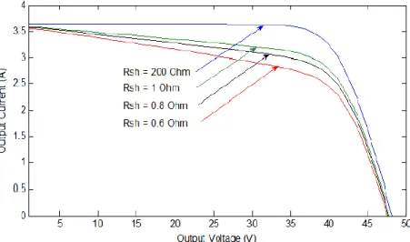
has no effect on the PV cell short circuit current, ISC, but it reduces the PV cell open circuit
voltage as shown in I-V characteristic and P-V characteristic in Fig. I.6 and Fig. I.7 respectively. Without leakage current to the ground the, RSh, can be assumed to be infinite. From Fig. I.7, it
can be seen that the maximum power point Pmax in the knee, increases with the increases of RSh
10
Fig. I.6 Effect of shunt resistance on the I-V characteristic
Fig. I.7 Effect of shunt resistance on the P-V characteristic
On the other hand, a small variation in RS leads to a reduction in the short-circuit current but
has no effect on the open-circuit voltage as in Fig. I.8, therefore the maximum power changes significantly as depicted in Fig. I.8 and Fig. I.9 [14].
11
Fig. I.8 Effect of series resistance on the I-V characteristic
Fig. I.9 Effect of series resistance on the P-V characteristic
I.6 Photovoltaic cell appropriate model
As mentioned above, the small variation in RS has a significant effect on the output power of
the PV panel. On the other hand, the PV efficiency is insensitive to the variation in RSh, which
can be assumed to approach infinity without leakage current. Therefore, the RSh can be
neglected to give the appropriate model with suitable complexity. And the effect of RSh on the
I-V characteristic and P-V characteristic of the PV array is shown in Fig.I.6 and Fig.I.7
respectively [13]. Neglecting the shunt resistance, the model of PV cell becomes an appropriate model with suitable accuracy as shown in Fig. I.10 and Equation (I.6) can be written as:
𝐼𝑃𝑉 = 𝐼𝑃ℎ− 𝐼𝑆⋅ [(
𝑞 ⋅ (𝑉𝑃𝑉 + 𝐼𝑃𝑉⋅ 𝑅𝑠)
12
The value of RS is provided in the datasheet by some manufactures. However, if is not provided,
the equation of RS can be derived by differentiating the Equation (I.7) and rearranging in terms
of RS. 𝑑𝐼𝑃𝑉 = 0 − 𝐼𝑠 ⋅ 𝑞 ( 𝑑𝑉𝑃𝑉+ 𝑅𝑆⋅ 𝑑𝐼𝑃𝑉 𝐴 ⋅ 𝑘 ⋅ 𝑇𝐶 ) ⋅ 𝑒 𝑞(𝑑𝑉𝑃𝑉+𝑅𝑆⋅𝑑𝐼𝑃𝑉 𝐴 . 𝑘 . 𝑇𝐶 ) (I.8) 𝑅𝑆 = −𝑑𝐼𝑃𝑉 𝑑𝑉𝑃𝑉− 𝐴 . 𝑘 . 𝑇𝑐⁄𝑞 𝐼𝑆. 𝑒𝑞( 𝑉𝑃𝑉+𝑅𝑆.𝐼𝑃𝑉 𝐴 . 𝑘 . 𝑇𝐶 ) (I.9)
Then by evaluating the Equation (I.9) under the open circuit voltage condition when VPV =
VOC and IPV = 0. 𝑅𝑆 = −𝑑𝑉𝑃𝑉 𝑑𝐼𝑃𝑉|𝑉 𝑂𝐶 − 𝐴 . 𝑘 . 𝑇 𝑐⁄𝑞 𝐼𝑆. 𝑒𝑞(𝐴 . 𝑘 . 𝑇𝑉𝑂𝐶 𝐶) (I.10) In Equation (I.10); 𝑑𝑉𝑃𝑉
𝑑𝐼𝑃𝑉
|
𝑉𝑂𝐶is the slope of the I-V curve at the VOC.Fig. I.10 Appropriate equivalent circuit model
It is possible for the Equation (I.7) of I-V characteristics to be solved. However, the inclusion of a series resistance in the model makes finding a solution complex. Although the answer can be found by using Newton’s method [9].
The Newton’s method is described as follows: 𝑥𝑛+1 = 𝑥𝑛− 𝑓(𝑥𝑛)
13
f '(x) is the derivative of the function, f (x) = 0, xn is present value, and xn+1 is a next value.
Rewriting the Equation (I.7) yields the following equation: 𝑓(𝐼𝑃𝑉) = 𝐼𝑃ℎ− 𝐼𝑃𝑉− 𝐼𝑆⋅ [𝑒𝑥𝑝 (
𝑞 ⋅ (𝑉𝑃𝑉+ 𝐼𝑃𝑉. 𝑅𝑠)
𝐴 ⋅ 𝑘 ⋅ 𝑇𝐶 ) − 1] = 0 (I.12)
Substituting Equation (I.12) into (I.11) yields the following equation, and the output current IPV
is computed iteratively by using Newton’s equation
𝐼𝑃𝑉(𝑛+1) = 𝐼𝑃𝑉(𝑛)− 𝐼𝑃ℎ−𝐼𝑃𝑉(𝑛)−𝐼𝑆 ⋅ [ 𝑒𝑥𝑝 ( 𝑞 ⋅ (𝑉𝑃𝑉+ 𝐼𝑃𝑉(𝑛)⋅ 𝑅𝑠) 𝐴 ⋅ 𝑘 ⋅ 𝑇𝐶 ) − 1] −1 − 𝐼𝑆 . ( 𝑞 ⋅ 𝑅𝑆 𝐴 ⋅ 𝑘 ⋅ 𝑇𝑐) . 𝑒𝑥𝑝 ( 𝑞. (𝑉𝑃𝑉+ 𝐼𝑃𝑉(𝑛) ⋅ 𝑅𝑠) 𝐴 ⋅ 𝑘 ⋅ 𝑇𝐶 ) (I.13)
By using MATLAB/Simulink, the Characteristics of I-V functions can be computed using Simulink program in Fig I.11
Fig.1.11Simulink program of the IPV -VPV characteristic curve of GPV generator panel solar.
The electrical performance of the solar cell is always described by two factors, the short circuit current ISC and the open circuit voltage VOC. The ISC is the point where the curve intersects with
14
This is measured by connecting the positive and negative terminals of the cell together. When the terminals are shorted the output voltage of the circuit is zero.
VOC is the point where the curve intersects with the horizontal axis and represents the maximum
possible output voltage from the circuit. This occurs when the PV cells are connected to a very large resistance or in case of no load. Under the condition of open circuit the current is zero. The power drawn by the photovoltaic module at any point along the curves are shown in Fig. I.6 and Fig. I.8 is expressed in watts. Since the voltage is zero under a short circuit current condition and the current is zero under the open circuit, the output power will be zero at these points.
I.7 Fill factor (FF)
The fill factor of photovoltaic generator is defined as the ratio of output power at MPP to the power result from multiplying VOC by ISC as in the Equation (I.15). It determines the shape
of the photovoltaic generator characteristic as shown in Fig.I.12. The fill factor plays an im-portant role when comparing the performance of different photovoltaic cells. A high fill factor is equal to a high quality cell which has low internal losses.
𝐹𝐹 = 𝐼𝑀𝑃𝑃∙ 𝑉𝑀𝑃𝑃𝐼𝑆𝐶∙ 𝑉𝑂𝐶 = 𝐴𝑟𝑒𝑎 𝐵 𝐴𝑟𝑒𝑎 𝐴 (I.14)
After simple multiplication the following equation results
𝐼𝑆𝐶 ∙ 𝑉𝑂𝐶 𝐹𝐹 = 𝐼𝑀𝑃𝑃 ∙ 𝑉𝑀𝑃𝑃 = 𝑃𝑚𝑎𝑥 (I.15)
Where IMPP is the current at MPP and VMPP is the voltage at MPP. The fill factor ranges from
material to material and it can be seen that it is always < 1. The closer the fill factor is to unity the better the operation of PV cell. The factors which affect (FF) are the shunt and series re-sistances of the photovoltaic generator as shown above in Fig.I.6 to Fig. I.9. A good fill factor is between (0.6-0.8) [7].
15
Fig. I.12 Photovoltaic module characteristics showing the fill factor.
I.8 Effect of temperature
The panel temperature is considered one of the important parameters due to its effect on the output power of photovoltaic panel [10, 11].
Fig. I.13 Effect of temperature on the I-V and P-V characteristic at constant irradiance.
The open circuit voltage VOC is highly influenced by the increase in the panel temperature as
shown in the Fig. I.13. As the temperature increases with a fixed irradiation level it results in a slight increase in the short circuit current ISC, because the band gap energy decreases and more
16
temperature have an obvious reduction in the PV panel output power due to the drop in the open circuit voltage VOC and the fill factor; therefore the module efficiency is reduced [1].
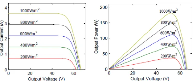
I.9 Effect of irradiation
At constant temperature the change in irradiation has a clear effect on the PV output max-imum power as illustrated in Fig. I.14 [10,11]. It is obvious that as the irradiation level increases the PV output voltage and current increases with it. In general, the increment in the irradiation level leads to a theoretical increment in the maximum power voltage when there is no change in the cell temperature. On the other hand, the short circuit current ISC depends totally and
line-arly on the irradiance level; therefore the maximum power current is changed as shown in Fig. I.14 [11].
Fig. I.14 Effect of irradiance on the I-V and P-V characteristic at constant temperature.
I.10 PV module and array module
The typical output power of solar cells in general is very low. It is normally less than 2W at 0.5V. Therefore, the photovoltaic cells are connected in particular configurations so as to form an array which is called a photovoltaic module. In general, the modules consist of group of cells connected in series and parallel to provide the desired output power and voltage as depicted in Fig. I.15. In addition to that, for a photovoltaic system a group of several PV mod-ules are connected in parallel and series in form of PV array to generate the required voltage and current values for the system. When two or more solar panels are wired in series, the same current flows through each panel and the output voltage is the sum of the voltages generated by each panel. Hence, Equation (I.7) can be written as
17 𝐼𝑃𝑉 = 𝑁𝑃. 𝐼𝑃ℎ− 𝑁𝑝. 𝐼𝑆 . [exp ( q A ⋅ K ⋅ TC ( VPV NS + IPV⋅ RS NP)) − 1] (I.16)
In contrast, when the solar panels are wired in parallel the output current becomes the sum of the currents from each panel, and the output voltage remains the same.
Fig. 1.15 Solar model in parallel and series branches.
I.11 Solar I-V characteristics with resistive load
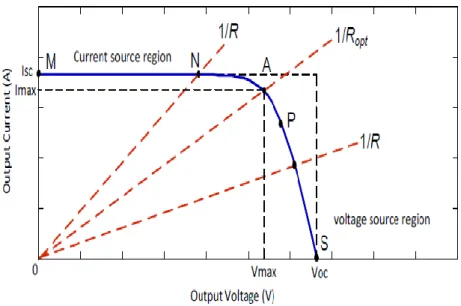
As can be seen in Fig. I.16 and I.17, the simulation program and the operating characteristic of a solar cell consists of two main regions: the voltage source region and current source region. The voltage source region is located at the right of I-V curve and the internal impedance of the solar cell in this region is low. Where the current source region is located on the left of the I-V curve and the internal impedance in this region is high. Additionally, it can be observed from the I-V curve, that the output current remains almost constant while the terminal voltage changes in the current source region. But in the voltage source region over wide range of output current the terminal voltage has only slight changed.
18
Fig. I.16 Simulink program of PV with resistive load=Rc
Fig. I.17 Intersection of the IPV -VPV characteristic curve and the load characteristic.
I.12 Interfacing the PV array to the load through DC-DC converter
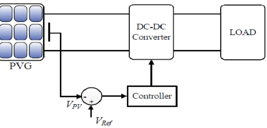
This section presents how to maximize the power delivered from the PV array to the load at all insolation levels. A buck converter with the output filter, which is essentially a step-down converter, also known as a chopper, inserted between the PV array and the load as shown in Fig. I.18 is a solution to transfer the maximum power.
19
Fig. I.18 PV array supplying R load through step-down converter.
In block diagram shown above, the maximum power can be transferred to the load by the chopper when it is driven with optimal duty ratio D. The peak power Ppeak delivered to the load under steady-state conditions at any solar insolation levels can be derived.
When a fixed resistive load (R) is connected directly to the PV cell’s terminals, the operating point is determined by the intersection of the solar cell I-V characteristic with the I-V charac-teristic of the load. As shown in the Fig. I.17, the characcharac-teristic of the resistive load is a straight line with a slope, I/V =1/R [12, 13]. Additionally, the power delivered to the load depends only on the resistance value. If the load resistance is small, the cell operates in the current source region MN of the curve, almost near to the short circuit current. Alternatively, if the load re-sistance is large, the cell operates on the voltage source region PS of the curve, almost near to the open circuit voltage [14].
From Fig. I.16 it is clear that, the operating point may not be at the point (A) which is the maximum power point (MPP) of the PV array. Furthermore, the output characteristics of PV cells are nonlinear, and the optimum operating point constantly varies with changes in the en-vironmental conditions of solar irradiation and cell temperature. The effects of solar irradiation and cell temperature on the P-V and I-V characteristics are shown in Fig. I.12 and Fig. I.13 respectively.
Since the MPP depends on factors that are not constant and cannot be controlled, i.e. solar irradiation and temperature, a device capable of tracking the MPP and maintain the operation at this point is needed. A maximum power point tracker is a device capable of tracking the MPP, and this device consists of DC-DC power converter its duty cycle adjusted by MPPT controller will be discussed at the next chapter.
20 I.13 Summary
In this chapter, the model development for the component parts of the proposed PV system are discussed. It begins with the physical structure of PV cells along with the fundamental concept and principles of converting the solar energy to electrical energy. The modeling of equivalent electrical circuit of PV cell presented and discussed. The model is implemented using MATLAB/SIMULIN to study the PV characteristics. Furthermore, the low output power of the single cell is discussed and how to connect number of cells in series and parallel to form a PV panel and array to meet the desired load power. The effect of temperature and solar radiation on the I-V and P-V characteristics of PV cell also discusses this chapter to show the importance of MPPT in the PV system.
21
Chapter II: Maximum power point tracking
techniques and DC-DC converters
II.1 Introduction
The main objective of maximum power point tracking is to read the voltage and current from the solar panel, perform the calculation for power and then display the power at its maximum. There are many algorithms available to execute this process. Some examples include Perturb and Observe (P&O), Incremental Conductance, Parasitic Capacitance and Constant Voltage Method. Of all the available algorithms, P&O is the most widely used algorithm because of its easy implementation. As for the Incremental Conductance method, it is more complex. However, a pro with this method is that it can be more accurate than the P&O method. For this project, P&O method was chosen to perform the MPPT algorithm. The output voltage and current from the solar panel constantly feeds the input of the DC/DC converter. Since the type of DC/DC converter chosen for this project is the buck converter, it will step the input voltage down based on the duty cycle. The preset duty cycle for the simulation is 70%, so the voltage from the input of the buck converter will be reduced when measure the output of the panel solar.
The output voltage and current of the panel solar sampled and then calculated for power. The calculated power then gets compared to the previous maximum power, if there is one. For the comparison, if the current power is greater than the previous maximum power and the current voltage is also greater than the previous voltage, then the converter’s duty cycle increases. Likewise, if the current voltage is less than previous voltage then the duty cycle decreases. As for the case that current power is less than the previous power, and the current voltage is greater than the previous voltage, according to P&O algorithm, the duty cycle of the buck converter should decrease. However, if the current voltage is less than the previous voltage, then increase the duty cycle. The process described above is in one loop of the code. Before starting the next loop, the current power is set to the previous power if it is greater than the previous power. Then a new loop of the same process which is by starting to measure the new voltage and current that is resulted from the newly set duty cycle of the buck converter.
II.2 Maximum power point tracking (MPPT)
It is very important with photovoltaic generation to operate the system at high power efficiency by ensuring that, the system is always working at the peak power point regardless of
22
changes in load and weather conditions. In other words, transfer the maximum power to the load by matching the source impedance with the load one. To confirm that, an MPPT system has been implemented which enables the maximum power to be delivered during the operation of the solar array and which tracks the variations in maximum power caused by the changes in the atmospheric conditions.
The MPPT system is basically an electronic device inserted between the PV array and the load. This device comprises two essential components, as illustrated in Fig.II.1. A DC-DC switching power converter along with an MPPT control algorithm to operate the PV system in such way it can transfer the maximum capable power to the load.
Fig. II.1 Converter acting as a Maximum Power Point Tracker.
As the solar panel outputs power, its maximum generated power changes with the atmospheric conditions (solar radiation and temperature) and the electrical characteristic of the load may also vary. Thus, the PV array internal impedance rarely matches the load impedance. It is crucial to operate the photovoltaic generation system at the MPP or near to it to ensure the optimal use of the available solar energy. The main objective of the MPPT is to match these two parameters by adjusting the duty ratio of the power converter. As the location of the MPP on the I-V curve varies in an unpredictable manner it cannot be defined beforehand due to changes of radiation and PV panel temperature. Accordingly, the use of MPPT algorithm or calculating model is required to locate this point [5].
There are several methods to track the MPP of the photovoltaic system that have been carefully studied, developed and published over the last decades. The authors in [5] have presented many MPPT control algorithms, some of which are addressed in the following sections. There are variations between these techniques in terms of, simplicity, sensor requirements, cost, range of efficiency, convergence speed and hardware implementation. Some MPPT algorithms outperform the others under the same operating conditions. A review and analysis of several
23
MPPT techniques have been carried out in [2] to quantify the performance of each control algorithm compared to the others.
II.3 Performance specifications of MPPT control algorithm
As noted earlier, the dynamic response, steady-state error and tracking efficiency should be considered for a successful design when evaluating the performance of a new or modified MPPT control algorithms [3].
II.3.1 Dynamic response
The response of a MPPT control algorithm needs be fast to track the MPP during the rapid changes in the atmospheric conditions (solar irradiation and temperature). The higher the tracking speed of the MPPT algorithm, the lower the loss in solar energy in the system.
II.3.2 Steady-state error
The MPPT control algorithm should stop tracking, once the MPP is located and should force the system to maintain operation at this optimal operating point as long as possible. However, this is impossible to achieve practically in an actual MPPT system because of the active perturbation process in MPPT algorithms with fixed tracking step-size and the continuous variation in solar insolation and temperature. This phenomenon has a negative impact on the PV system efficiency.
II.3.3 Tracking efficiency
Defining the tracking efficiency is a very important step, to quantify how successfully an MPPT control algorithm tracks the MPP and to what extent it contributes to increase the overall performance of the PV system compared to other methods. According to [4,5] the tracking efficiency is defined as the ratio between the actual power of the PV array and the theoretical power during the same time period. The atmospheric conditions (irradiation and temperature) are changeable and vary over a wide range. Hence, each MPPT algorithm must be evaluated over a range of different operating conditions when comparing MPPT algorithm performance. A well-designed MPPT control system should provide good performance in different atmospheric conditions.
II.4 MPPT algorithms classification
Several MPPT algorithms have been proposed for PV power systems in recent years, to locate the MPP and increase the system efficiency. The MPPT algorithms may be divided into two types, which are indirect control or “quasi tracking techniques” and direct control or “true tracking techniques” [5, 6]. In the indirect control techniques, the MPP is calculated either
24
by measuring the voltage and current of the PV array, the solar insolation, or by the use of mathematical functions obtained from empirical data. Therefore, these techniques are incapable of tracking the MPP with varying irradiation and temperature. The indirect control techniques are look-up table technique, constant voltage technique, fractional open-circuit voltage and fractional short-circuit current. However, the true tracking techniques have the ability to find the optimum operating point even under changing atmospheric conditions, because they do not rely on previous knowledge of or calculated data from the PV array V-I characteristics. The true tracking techniques are the perturbation and observation (P&O) technique, incremental conductance (INC) technique and others techniques. In the tracking process one or two variables are used for calculating the MPP. The fractional open-circuit voltage and fractional short-circuit current use only one variable, either the PV array output voltage or current respectively, though the P&O need both variables to determine the MPPT [5, 6] Fig II.2.
Fig. II.2 Schematic block diagram of the load-matching method.
II.4.1 Constant voltage method (CV)
If the PV system is implemented without a load (battery) to tie the bus voltage to an approximately constant level, a simple control scheme of the constant voltage method can be applied as presented in [6, 7]. In this method the feedback of the PV voltage is compared with a fixed reference voltage and the resultant signal adjusts the duty ratio of the DC-DC converter to keep the operating point of the PV array at the MPP or close to it, as illustrated in Fig. II.3. The reference voltage is set to be equal to the VMPP of the characteristic PV array or to another
25
Fig. II.3 Voltage feedback MPPT method with constant voltage reference.
This method is simple, economical and only one feedback-loop control is required. However this technique has the drawback that it does not correct for environmental variation such as change in irradiation and temperature [5].
II.4.2 Perturb and observe (P&O) algorithm
The perturb and observe algorithm is considered to be the most commonly used MPPT algorithm among the other techniques because of its simple structure and ease of implementation. It is based on the concept that on the power-voltage curve, the change in the PV array output power is equal to zero (ΔPPV = 0) on the top of the curve as illustrated in Fig.
2.4 [8]. The P&O operates by periodically perturbing (incrementing or decrementing) the PV array terminal voltage or current and comparing the corresponding output power of PV array
P(n +1) with that at the previous perturbation P(n) . If the perturbation in terminal voltage leads to increase in the PV power (ΔPPV > 0) the perturbation should be kept in the same direction,
otherwise the perturbation is moved to the opposite direction. The perturbation cycle is repeated until reaching the maximum power at (ΔPPV = 0). The control flow chart of P&O is shown in
Fig. II.5. There are two different ways to implement the P&O algorithm. In the conventional way a reference voltage is used as a perturbation parameter; therefore a PI controller is needed to adjust the duty ratio. The second way is that, the duty ratio is directly perturbed and the power is measured every PWM cycle. The advantages of this technique are simplicity, ease of implementation and it does not require a previous knowledge of the PV array.
However, the P&O will not stop perturbing when the MPP is reached and will oscillate around it resulting in some unnecessary power loss.
26
Fig. II.4 Sign of the dP/dV at different positions on the power characteristic.
27 II.5 DC-DC converters
The switch mode DC-DC converter is considered the main part of a MPPT system. These are widely used to convert unregulated DC inputs into a controlled DC output at a desired voltage and current levels in DC power supplies and DC motor drives. The same converter is used for a MPPT to provide load matching for the maximum power transfer by regulating the input voltage at the PV array MPP by controlling the duty ratio (D).
If the photovoltaic panel is directly connected to a load, its operating point will be defined by the intersection of the load and photovoltaic generation curves as shown in Fig. I.15. Therefore, there is a unique point where the both curves intersect each other, exactly at a MPP. The generation curve nonlinearly changes with the change of the radiation (G) and temperature (T), while the load curve has a different characteristic according to the type of load is connected to the photovoltaic module. Hence, DC-DC converters are used to interface the photovoltaic module with the load, in order to ensure the photovoltaic module is always operating at the maximum power point. This is done by controlling the converter duty ratio (D) with maximum power point tracking algorithms (MPPT).
II.5.1 Topologies
There are several types of DC-DC converters. They are generally categorized into two types: isolated and non-isolated converters. In the isolated topologies a small high frequency electrical isolation transformer is used to provide the DC isolation between the input and output of the DC converter; and step up or down of the output voltage is achieved by changing the transformer turns ratio. These types of converter are used in switch mode power supply [99]. The flyback, half bridge and full bridge are the most commonly used topologies for majority of the applications [5]. Also these types of topology are used in PV grid-tied system when electrical isolation is needed for safety reasons, and to eliminate the possibility of coupling DC to AC grid.
Non-isolated converters do not have an isolation transformer. They are very often used in DC motor drives [7]. Non-isolated converters are classified into three types: step up (boost), step down (buck), and step up & step down (buck-boost).
II.5.2 Buck converter
In this type of DC-DC converter, the average output voltage Vo produced is always lower
28
such as for charging batteries and in water pumping systems. The basic circuit of the step-down converter as illustrated bellow in Fig. II.6 [7]. The diode (d) is used to enhance the output filtering effect and prevent the switch from absorbing or dissipating the inductive energy because this would lead to overheating the switch. In addition to that, there is an inductor and capacitor at the output of the converter which forms a low-pass filter to attenuate the output voltage fluctuation.
Fig. II.6 Step-down Buck converter.
Fig. II.9 illustrate the wave forms of the inductor current (iL) and voltage (vL) of the step-down
converter operating in a continuous conduction mode.
Fig. II.7 Step-down Buck converter switch closed.
At the time duration when the switch S is on as shown in Fig. II.7, the diode d becomes reverse biased and the input voltage Vd appears across the inductor leading to linear increase in the
29
Fig. II.8 Step-down Buck converter switch open.
When the switch S is turned off as shown in Fig. II.8, the diode d becomes forward biased and the voltage across the inductor is reversed vL = -Vo. Therefore, current in the inductor freewheel
through the diode and starts decreasing linearly. In this cycle the capacitor is charged by the inductor energy.
Fig. II.9 Step-down converter wave form of the inductor current and voltage in continuous current mode.
The waveform must repeat from one time period to the next during steady-state operation. The relation between the input and output voltage, input and output current and the duty ratio D can be defined by Equation (II.1) and (II.2) [9].
𝑉𝑜 𝑉𝑑 = 𝑡𝑜𝑛 𝑇𝑠 − 𝐷 (II.1) 𝐼𝑜 𝐼𝑑 = 1 𝐷 (II.2)
30 𝐿 =𝑉𝑆(1 − 𝐷)
2ΔI𝑆 𝑓𝑆 (II.3)
𝐶 = 𝐼𝑜𝐷
8ΔV𝑜 𝑓𝑆 (II.4)
In Equations (II.1) and (II.2) TS is the switching period, or time period of square pulse that
controls the electronics switch S, ton is the on time of controlling square wave, Io is the converter
output current, Id is the converter input current.
II.5.3 Boost converter
Example applications of boost converter operation are the regenerative braking circuit of DC motors and in regulated DC power supplies. In this type of converter the output voltage is always greater than the input voltage. Therefore the step up converter can be applied to MPPT systems where the output voltage needs to be greater than the input voltage. Such as in a grid-connected system where the boost converter maintains a high output voltage even if the PV array voltage falls to low values. The circuit topology of the step-up converter as illustrated in Fig. II.10 [8].
Fig. II.10 Step-up boost converter.
When the switch S is on the diode d is reverse based. Consequently, the current in the inductor
L rises linearly due to the input voltage source, and in this case the output stage is isolated and
the capacitor C is partially discharged supplying the current load. When the switch is off during the second interval the diode is conducting, and during this time the output stage receives energy from both the inductor and the input source. The wave form of the inductor current during
31
continuous conduction mode is shown below in Fig. II.11 where the inductor current flows continuously, i.e. IL(t) > 0 [8,9].
When the converter is operating at steady-state condition, the duty ratio, D, can be expressed by Equation (II.5) [9].
𝐷 = 1 −𝑉𝑑
V𝑜 (II.5)
Fig. II.11 Step-up converter wave form of the inductor current and voltage in continuous current mode.
Where D denotes the duty ratio, Vd and Vo denotes the input and the output voltages of the
converter, respectively. From the above equation it can be seen that, the increase in the duty ratio D will increase the value of the output voltage, Vo. In addition the change in the duty ratio
results in change in the input and the output current of the converter. The filter inductor and capacitor to operate the converter in the continuous conduction mode can be calculated by the following equations:
𝐿 = 𝑉𝑑𝐷
2ΔI𝐿𝑓𝑠 (II.6)
𝐶 = 𝐼𝑜𝐷
32 II.5.4 Buck-Boost converter
A Buck-Boost converter is cascade connection of two basic converters, the buck converter and boost converter. The Buck-Boost converter provides an output voltage can be higher or lower than the input voltage. Also this type of converter produces a negative polarity output with respect to the common terminal of the input voltage [7]. The main application of Buck-boost converter is in regulated DC power supplies. Fig. II.12 shows the circuit topology of Buck-Boost converter [8, 9].
Fig. II.12 Buck-boost converter.
In the equivalent circuit shown in Fig. II.12 when the switch S is turned on during the first time interval ton of the switching period TS, the diode d is reverse based and input provides energy to
the inductor causing the inductor current iL to increase as illustrated in Fig. II.13. When the
switch is off during the second time interval toff, the diode is forward biased so the energy stored
in the inductor is transferred to the load. In this case the inductor current iL is forced to flow
backwards through the load and results in a negative polarity in the converter output voltage.