Centre de Recherche en économie de
l’Environnement, de l’Agroalimentaire, des
Transports et de l’Énergie
Center for Research on the economics of the
Environment, Agri-food, Transports and
Energy
_______________________
Barla: Corresponding author. CDAT-CREATE, Université Laval, Département d’économique, 1025, av. des Sciences-Humaines, Québec, QC, Canada G1V 0A6
Lapierre et Herrmann : CDAT-CREATE, Université Laval, Département d’économique, 1025 av. des Sciences-Humaines, Québec, QC, Canada G1V 0A6
Alvarez Daziano: School of Civil and Environmental Engineering, Cornell University, 305 Hollister, Ithaca, NY, USA 14853
Les cahiers de recherche du CREATE ne font pas l’objet d’un processus d’évaluation par les pairs/CREATE working papers do not undergo a peer review process.
ISSN 1927-5544
Reducing Automobile Dependency on Campus :
Evaluating the Impact TDM Using Stated Preferences
Philippe Barla
Nathanaël Lapierre
Ricardo Alvarez Daziano
Markus Herrmann
Cahier de recherche/Working Paper 2012-3
Reducing automobile dependency on campus: evaluating the
impact TDM using stated preferences
†
Philippe Barla
a, Nathanael Lapierre
a, Ricardo Alvarez Daziano
band Markus
Herrmann
aaCDAT-CREATE, Université Laval, Département d'économique, 1025 av. des sciences-humaines, Québec, QC, Canada G1V 0A6
b
School of Civil and Environmental Engineering, Cornell University, 305 Hollister, Ithaca, NY, USA 14853
Abstract
In this paper, we evaluate the potential impacts of travel demand management strategies to reduce the commuting mode share of automobiles using stated preference data. The analysis is carried out on members of Université Laval in Quebec City (Canada). We measure the impact of travel time and cost as well as attitudes toward automobile, public transit and the environment. We find elasticities with respect to time and cost parameters that are low implying that large changes are required to have a noticeable impact. We find however that combining several policy interventions is more effective. Policies aiming at reducing automobile dependency by changing attitudes do not appear to be particularly effective.
Keywords: mode choice; stated preferences; travel demand management
Résumé
Dans cet article, nous évaluons, à partir de données de type préférences déclarées, les impacts potentiels de stratégies de gestion de la demande de trafic visant à réduire la part modale de l’automobile dans les déplacements domicile-travail. L’analyse s’effectue sur les membres de la communauté universitaire de l’Université Laval à Québec (Canada). Nous mesurons l’effet du temps et du coût de déplacement ainsi que des attitudes face à l’automobile, le transport en commun et l’environnement. Nous trouvons des élasticités par rapport au temps et au coût qui sont faibles. Des changements importants dans la valeur de ces paramètres sont donc nécessaires pour avoir un certain effet sur la part modale de l’automobile. Nous trouvons cependant que la combinaison de plusieurs mesures semble nettement plus efficace. Par contre, des politiques qui visent à changer les attitudes ne semblent pas avoir beaucoup d’effet.
Mots clés: Choix modal, préférences déclarées, gestion de la demande de trafic
Classification JEL: R41, R48, Q58
1. Introduction
In this paper, we evaluate the potential for reducing the commuting mode share of cars at Université Laval (UL) in Quebec City (Canada) using stated preference (SP) data. Specifically, we investigate how students and staff that are presently driving at least three times a week to the University campus are shifting to public transit when the price and/or travel time of car and public transit are modified. We also explore to what extent changing attitudes toward car, public transit and the environment may be effective. Our investigation is of interest as many University campuses are trying to curb growing automobile dependency and its related negative externalities such as congestion, land degradation and air pollution. Moreover, Universities are ideal environments to evaluate the potential of travel demand management (TDM)
strategies as the population is relatively homogenous, well educated, easy to contact and, may be, more open to changes.
Several Universities are already implementing TDM strategies such as increasing prices and reducing supply of parking spaces, creating carpooling website or improving bicycle infrastructures (see Daggett and Gutkowski, 2003, Balsas, 2003). Education and outreach programs are also often part of the strategies to develop sustainable transportation habits. One of the most noticeable strategies has been the implementation of Universal Transit Pass (U-Pass) programs that provide students and sometimes staff unlimited free access to local transit. These programs are usually funded by an increase in registration fees paid by all students. Around one hundred Universities in North American have now a U-Pass program. Some studies have evaluated the impact of these TDM strategies on campus traffic. For example, Brown et al. (2003) evaluates the impact of the U-Pass program at the University of California, Los Angeles (see also Boyd et al., 2003). They compare the changes in modal shares before and after the implementation of the U-Pass program and compare it to a control group of students and staff that are not living nearby a bus line that is part of the U-Pass system. They find that the program did increase transit ridership by more than 50% during the first year while solo driving declined by 20%. The implied arc elasticities are -0.28 for the fare elasticity of transit demand and 0.1 for the cross-elasticity between transit fare and the number of solo drivers. Ubillos and Sainz (2004) estimate a transport demand function for university students in the Bilbao area using revealed preference data. They find surprisingly large price elasticity for public bus (-4) whereas the price elasticities for underground and train are small (less than -0.2). Reducing travel time and increasing service frequency of these last two modes represents an improvement in travel quality which affects their modal shares more importantly as compared to enhancing the travel quality of public buses. Closer to our empirical strategy, Albert and Mahalel (2006) examine the impact on automobilists of introducing either a congestion toll or a parking fee on the campus of the Israel Institute of Technology using SP data. They find high elasticities for both congestion and parking charges (respectively 1.8 and -1.2).
Several studies have also evaluated TDM policies using SP data in a context other than University campuses. For example, Washbrook et al. (2006) evaluates the impact of road and parking pricing on commuting automobile drivers in the Greater Vancouver suburban area. They find elasticities of drive-alone probability with respect to toll and parking-charges to be about -0.3. Espino et al. (2007) combine revealed and stated preference data to analyze the choice of mode (car-driver, car-passenger or bus) in suburban corridors in Spain. Their results also show that demand is more sensitive to travel time than cost but is inelastic with respect to all other parameters. In addition, the demand is more sensitive to policies that penalize cars than those improving bus with the exception of bus frequency.
Our paper is structured as follows. In section 2, we describe the UL and present the methodology, specifically the stated preference survey and the econometric modeling. The results and policy simulations are presented in sections 3 and 4 respectively. We conclude in section 5.
2. The methodology
Before describing the methodology, it is useful to briefly describe the UL context. The University has about 35 000 full time equivalent students and more than 5000 employees. The main university campus is located at about 6 km from Quebec City downtown. It can be viewed as an island of approximately 2 km2 in the middle of a suburb development dating back to the 1950s and 1960s. It is served by several bus routes, including many high-frequency buses. A bus trip costs 2.6$ but monthly bus passes are available at a cost of about 50$ for students and 70$ for the general public. About 8000 parking spaces spread over 50 different parking lots are available on campus. There are three categories of parking permits available which differ upon the localization of the authorized lots with respect to the University buildings. For each category, the parking permit price also varies upon its duration (e.g. one or two semester and annual). Based on the annual permit prices, the monthly cost varies from a low of 34C$ to a high of 68C$. UL generates more than 31 000 trips per day, making it the third most important destination in the area (see MTQ, 2008). The estimated modal shares are presented in table 1. Overall, the modal share of the automobile is close to 40% but with significant differences between the students and staff population.
their travel mode choice. In order to boost participation, each respondent had the opportunity to win a 500$ prize. Strict confidentiality was also guaranteed. Overall, 6120 individuals responded to at least one question implying a response rate of about 15%.
The survey questionnaire has two parts. The first part is designed for all UL members. It collects information on the actual mode choice, commuting time and habits, attitudes toward transportation issues and socio-economic characteristics. The second part only targets car drivers that i) commute at least three times a week and ii) have the option of using public transit (i.e. they declare that this mode is a feasible option for them). In this paper, we focus our analysis on the sub-sample of solo-drivers that never use public transit to commute to campus.1 Respondents are confronted to hypothetical mode choice decisions that are conditioned in part on their responses to the first part of the survey.
The choice set is between automobile and public transit.2 For public transit, we ask respondents to assume that a direct service exists (without any transfer) and that the service frequency is good (at least one bus per twenty minutes). The attributes and the three levels used are presented in table 2. Travel time by car is the total door-to-door estimates provided by the respondent. For travel time by bus, we set the current level at twice the travel time by car which corresponds roughly to the area average ratio. We use an efficient design in order to reduce to 9 the number of choices that each respond has to make (ChoiceMetric, 2010). The software Ngene was used to find a D-efficient design.3 A screenshot of an example of the SP choice question is presented in appendix 1.
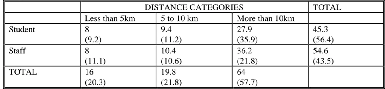
Our final sample includes 6220 choices made by 705 individuals. This number exceeds the minimum required sample size of 290 as derived by the S-estimate. Using information on parking permits sales, we find that our sample underrepresents students but is quite representative with respect to the distribution of the distance domicile-UL (see table 3). In any case, we use post-estimation weights to insure that our sample is representative with respect to these two dimensions.
The empirical modeling is based on the well-established random utility framework. The indirect utilities for automobile and public transit are respectively
𝑉𝐴𝑖= 𝛽0+ 𝛽1𝑇𝑖𝑚𝑒𝐴+ 𝛽2𝑇𝑖𝑚𝑒𝐴2+ 𝛽3𝑃𝑎𝑟𝑘 + 𝛽4𝑃𝑎𝑟𝑘 ∗ 𝐿𝑜𝑤𝑖𝑛𝑐+ 𝛽5𝑃𝑎𝑟𝑘 ∗ 𝑀𝑒𝑑𝑖𝑛𝑐+ 𝛽6𝑃𝑎𝑟𝑘2 + 𝐻𝑖′𝛽7 + 𝑍𝑖′𝛽8+ 𝜗𝑖+ 𝜀𝑎𝑖 ,
𝑉𝑇𝑖= 𝛼1𝑇𝑖𝑚𝑒𝑡𝑖+ 𝛼2𝑇𝑖𝑚𝑒𝑇∗ 𝑆𝑡𝑢𝑑𝑒𝑛𝑡 + 𝛼3𝑇𝑖𝑚𝑒𝑇2+ 𝛼4𝑇𝑖𝑚𝑒𝑇2∗ 𝑆𝑡𝑢𝑑𝑒𝑛𝑡 + +𝛼5𝐹𝑎𝑟𝑒 + 𝛼6𝐹𝑎𝑟𝑒 ∗ 𝐿𝑜𝑤𝑖𝑛𝑐+ 𝛼7𝐹𝑎𝑟𝑒 ∗ 𝑀𝑒𝑑𝑖𝑛𝑐+ 𝛼8𝐹𝑎𝑟𝑒2 + 𝜀𝑏𝑖 ,
with index A for the automobile and T for public transit. The variable 𝑇𝑖𝑚𝑒 measures total travel time. The specification search has led us to introduce this variable in quadratic form and to allow for the
coefficient to be alternative specific. Furthermore, the coefficients for the time variable in the public transit equation are allowed to be different for students. 𝑃𝑎𝑟𝑘 measures the cost of parking per trip and 𝐹𝑎𝑟𝑒 is the transit fee per trip.4 The coefficients on these two variables are allowed to vary depending upon the income group by including interaction terms with Low_inc (=1 if the income is below 20k) and Med_inc (=1 if the income is between 20 and 50k). The reference group corresponds to an income above 50k. 𝑃𝑎𝑟𝑘 and 𝐹𝑎𝑟𝑒 are also introduced in quadratic form.5
1
About 3% of solo-drivers declare using public transit as a secondary mode to commute to the campus.
2
Note that the questionnaire allows for the option of choosing a non-motorized mode for respondents that have declared that this is a feasible option for them (about 20%). However, less than 3% of respondents ever choose this mode in the hypothetical options we propose them. We therefore restrict our empirical analysis to the automobile-public transit decision. This simplification should not distort the analysis as the attributes of the non-motorized mode did not vary in the stated choice experiment.
3
The D-error is 0.00972.
4
For the automobile, we have tested specifications that include fuel costs estimates based on the distance driven and the make model and year of the respondent's car. The impact of this variable was not statistically significant, probably because of the lack of variability. Also, the impact of the other factors was not really affected. Moreover, one of the problems of this specification is that we are losing the observations for which the distance is not available.
5 Note that the design was derived using indirect utility functions that are linear in time and cost and that the design did
not include interaction terms or individual specific effects. The results obtained when using this simplified specification are however very close to those reported here.
𝐻𝑖 is a vector of three variables designed to help characterizing the attitudes of the respondents with respect to the automobile, public transit and the environment. Specifically, the variable Pro-auto indicates on a scale from 0 to 10 the respondent's level of agreement to the proposition ‘I could not live without a
car.’ The variable Pro-transit measures the level of agreement to the proposition ‘Developing public transit should be the first priority to reduce automobile dependency in the area’ and the variable Pro-Environment is the agreement with ‘My travel decisions are influenced by my concerns about climate changes and the quality of the environment.’ 𝑍𝑖 is a vector of variables describing the respondents
characteristics, travel habits and constraints. They are described in table 4. Even though we recognize that there is a very active research avenue in discrete choice modeling aiming at finding better ways of
integrating attitudinal constructs into discrete choice models (Ben-Akiva et al., 2002; Johansson et al., 2006; Daziano and Bolduc, 2011), we include in this paper the attitudinal effect indicators directly in the utility function as in Koppelman and Hauser (1978). In fact, we aim at exploring the overall effect of attitudes, since the main focus is targeted at the evaluation of TDM measures. In addition, note there are only three indicators making their direct inclusion in the model possible.6 In future research, we plan to explore more advanced modeling technics.
𝜗𝑖 are random variables that capture unobservable individual specific characteristics. They are assumed to be i.i.d. 𝑁(0, 𝜎𝜗2). 𝜀 are random variables that are i.i.d. Gumbel distributed. This specification
corresponds to a random-effects logit model that is estimated using the xtlogit procedure in Stata. Table 4 defines the variables and provides descriptive statistics corresponding to the current travel conditions.
3. The results
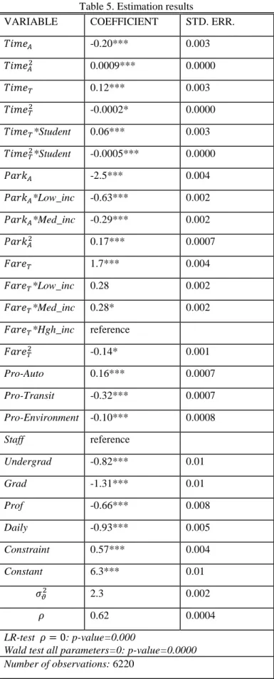
Table 5 reports the estimated coefficients and standard errors while table 6 shows the average elasticties and the implicit values of time saved. All the coefficients are statistically significant and have the expected sign. Also note that, a LR-test clearly rejects the null hypothesis of the absence of individual specific random effects. In fact, 62% of the error term variance is associated with the individual random components.7
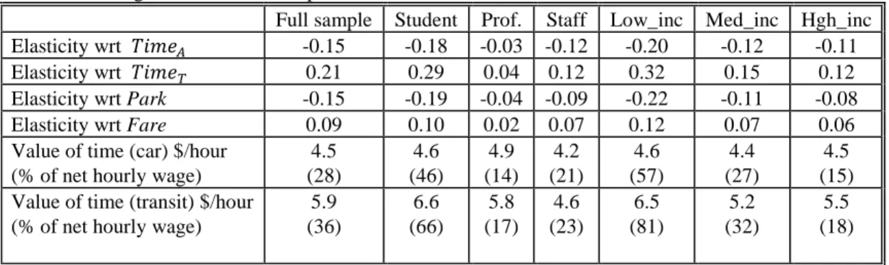
As travel time by car increases, the probability of choosing that mode declines. The average elasticity evaluated at current travel conditions is estimated at -0.15. Figure 1 shows, for an average respondent, how this elasticity is increasing in absolute value with the level of travel time by car. It reaches a value of -0.34 when travel time by car approaches the travel time by bus.8 From table 6, we also note that i) professors are much less sensitive to time travel by car and ii) the elasticity declines with income.9
As expected as travel time by transit declines, so does the probability of choosing to commute by car. The average elasticity is somewhat larger than for travel time by car at 0.21. Figure 2 shows that the elasticity is increasing as the travel time by bus declines so as to match the travel time by car which is set at about 30 minutes. The sensitivity to transit time is stronger for students and declines with income, i.e. for the groups that are more likely to switch mode.
The cost of parking lowers the probability of commuting by car. The average elasticity is low at -0.15 with clear difference across professional status and income groups. This value is about half the elasticity obtained by Washbrook et al. (2006). The elasticity is however increasing remarkably as the level of the parking charges is increased. Indeed, as figure 3 shows, it reaches a value of about -0.7 when the parking fee is doubled. Also, as expected, the sensitivity to the parking fee is stronger in lower income groups.
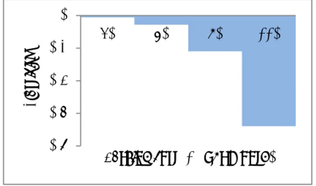
The impact of transit fare is even smaller with an average elasticity at 0.09. This value is however very close to Boyds et al. (2003). Once again the impact is somewhat larger for students and for the low income group. For an average respondent, the elasticity first increases, then declines as the bus fare level rises.
6
More general models use techniques of dimension reduction when the number of indicators is relatively large.
7
The individual effects improve the estimation of the probability of choosing the automobile under the current conditions (which should be 1) as well as in the various scenarios submitted to the respondent. For example, the sample average estimated probability under the current conditions is 0.96 when allowing for individual effects while it is 0.9 when these effects are excluded.
8
For the average respondent, the travel time by bus is set at the sample average value of 51 minutes.
9
The decline is due to the fact that the estimated probability of choosing the car becomes very close to unity as the fare level reaches 25C$ per month.10
The implicit values of time saved when driving acar are relatively low at less than 5$ per hour or about 30% of the estimated hourly net wage. Such a low values of time are not unusual with SP data as noted by Small and Verhoef (2007).11 We note little differences in the value across groups implying a sharp decline in the percentage of the wage from 57% to 15% for the low and high income group respectively. The value of time saved in public transit is somewhat larger but always less than 7$ or 36% of the hourly net wage. We observe here that students and low income groups are ready to pay a larger fraction of their wage. We have already noted above that these groups are more sensitive to travel time by transit than other groups. These groups are also those most likely to switch to public transit when this mode is improved.
The attitudinal variables 𝐻𝑖 also affect the probability of choosing the automobile. A rise by one unit for the variable Pro-auto increases the probability of driving by 0.5% while an additional unit for the variables
Pro-transit and Pro-Environment reduces this probability by 2.3% and 0.3% respectively. The impacts of
the 𝑍𝑖 variables are as follows. Compared to respondents that are part of the University staff, professors have a probability of solo-driving that is increased by 1.05%, while the probability is reduced by 2.5% and 8.5% for undergraduate and graduate students respectively. Daily commuters have a probability of driving reduced by 2.4%. These commuters are likely to have more stable schedules which may favor public transit. Respondents facing family, scheduling or itinerary constraints have a probability that is 1.8% higher to choose the automobile.
4. Evaluation of policies promoting public transit
In this section, we evaluate the potential for substitution from the automobile to public transit using different TDM instruments. The impacts are estimated using sample enumeration. For each respondent, we use the estimated parameters to compute the probability of choosing the automobile given the policy intervention. A weighted average probability is then obtained using the sample weights which is then compared to the weighted average probability without the policy intervention (status quo). We examine the following policies:
• [1] Free Transit: This policy represents free access to public transit for all members of the university community. Operationally, it is simulated by setting the transit fare to zero when estimating the probabilities.
• [2] Parking cost +60%: this policy would result in an increase of the average annual parking charges at the university from 660$ to 1056$ thereby roughly matching the parking cost at several parking lots around the University. It is simulated by increasing each respondent actual parking cost by 60%.
• [3] Equal time for transit and cars: in this scenario, we compute the change in mode choice associated with an improvement in public transit so that total travel time becomes identical to the actual travel time by car.
• [4] Combination of [1] & [2]: this policy corresponds to the simultaneous implementation of free transit and 60% increase in parking fees.
• [5] Combination of [1] & [3] • [6] Combination of [1],[2] and [3]
• [7] Attitudinal changes: in this scenario we try to evaluate the potential for modal shift through educational and outreach programs which would affect our three attitudinal variables. It is obviously difficult to predict to what extend this type of programs could effectively change attitudes, so we simply assume that they are able to change by 50% the value of each respondent's attitudinal variables. Specifically, they reduce the value of Pro-auto by 50% (with a floor at 0) and increase by 50% the value of Pro-transit and Pro-Environment (with a ceiling at 10).
10
The value of this elasticity is function of the term (1-𝑝̂) with 𝑝̂ the estimated probability of choosing the automobile.
11
Table 7 presents the results in terms of % reduction in the modal share of automobile. First, we find that offering a U-pass system would encourage 18% of solo drivers to switch to public transit. The impact is quite similar across respondent categories except for professors. Interestingly, this is very close to what Boyd et al. (2003) has observed after the implementation of the U-pass system at UCLA. The 60% hike in parking fee or matching transit and car travel time would reduce commuting driving by 10%. We therefore find that despite important changes in travel conditions, the reduction in automobile use is limited. However, it appears that combining several measures may be much more effective. Indeed, the decline in the share of automobile is around 50% when two instruments are combined which is more than the sum of each measure taken separately. It reaches more than 80% when all three measures are jointly implemented which is more than twice the cumulated change of [1], [2] and [3]. It goes without saying that implementing these three measures would be ambitious and could be costly particularly measure [3]. Finally, the impact of changes in attitudes (policy [7]) is quite limited with a reduction of only 4% in the probability of driving.
Note that some of these results may be somewhat overestimated as we do not consider the possibility for drivers to switch between parking permit categories when their prices increase. This option was indeed explicitly excluded in our hypothetical scenarios. In reality, it is very likely that some drivers would simply switch to a cheaper parking permit when faced with a parking fee hike. Also, recall that our hypothetical scenarios assume that commuting by transit entails no transfer and the level of service is at least two buses per hours. Since this level of service is not available for every respondent, our simulated impacts may be overestimated. However, the impacts may also be underestimated as they do not include the long-term effects of the policies on the decision to own a car, an aspect which may be particularly relevant for the student population. It also does not include the potential impacts on the residential location choice.
5. Conclusions
In this paper, we examine to what extent solo-driver commuters switch to public transit when travel time, cost conditions or attitudes are modified. The analysis uses the results of a stated preference survey carried out on the University Laval population. The main findings of our analysis are:
• It is important to take into account respondent-specific unobservable effects.
• All time and cost elasticities at current conditions are low varying between 0 and 0.3. These values are in the lower part of what has been found elsewhere in the literature.
• The implicit values of time saved are also quite low representing about a third of net wage. While the values vary little across groups, the share in terms of net wage varies quite a bit.
• Large changes in travel conditions are needed to significantly reduce solo driving.
• Combining several measures appear to be much more effective for reducing automobile dependency.
• Changing attitudes toward the automobile, public transit and the environment do not appear to be very effective in changing modal shares.
• Some differences exist between respondents based on their professional status and income group but these differences are not sufficient to affect the relevance of the above conclusions for each sub-group.
Table 1. Modal shares for commutes to UL (in % of trips)*
MODE TOTAL STUDENTS STAFF
Car-driver 33.7 22.8 58.4
Car-passenger 4.2 3.6 5.7
Bus 33.5 38.1 23.1
Active modes 28 35.1 12
* Based on our survey's results
Table 2. Attributes and level used in the stated choices
MODE ATTRIBUTES LEVEL 1 LEVEL 2 LEVEL 3
Automobile Travel time Current level 25% higher 50% higher
Parking cost Current level 50% higher 100% higher
Bus Travel time Current level* 25% lower 50% lower
Fare Current level 50% lower Free
*
estimated at twice the travel time by car.
Table 3. % of respondents in the sample by status and distance categories (in parenthesis % in the population based on parking permit sales information)
DISTANCE CATEGORIES TOTAL
Less than 5km 5 to 10 km More than 10km
Student 8 (9.2) 9.4 (11.2) 27.9 (35.9) 45.3 (56.4) Staff 8 (11.1) 10.4 (10.6) 36.2 (21.8) 54.6 (43.5) TOTAL 16 (20.3) 19.8 (21.8) 64 (57.7)
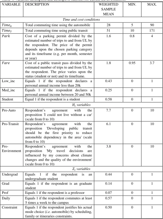
Table 4. Variables description and descriptive statistics for current travel conditions
VARIABLE DESCRIPTION WEIGHTED
SAMPLE MEAN
MIN. MAX.
Time and cost conditions
𝑇𝑖𝑚𝑒𝐴 Total commuting time using the automobile 28 5 90
𝑇𝑖𝑚𝑒𝑇 Total commuting time using public transit 51 10 171
𝑃𝑎𝑟𝑘 Cost of a parking permit divided by the estimated number of trips to and from UL by the respondent. The price of the permit depends upon the chosen parking category and its timeframe (e.g. per month, semester or year)
1.6 0.8 4
𝐹𝑎𝑟𝑒 Cost of a public transit pass divided by the estimated number of trips to and from UL by the respondent. The price varies upon the status (student or not) and its timeframe.
1.8 0.95 3.7
Low_inc Equals 1 if the respondent declares a personal annual income less than 20k
0.43 0 1
Med_inc Equals 1 if the respondent declares a personal annual income between 20 and 50k
0.25 0 1
Student Equal 1 if the respondent is a student 0.58 0 1
𝐻𝑖 variables Pro-Auto Respondent’s agreement with the
proposition 'I could not live without a car' (scale from 0 to 10)
7.7 0 10
Pro-Transit Respondent’s agreement with the proposition 'Developing public transit should be the first priority to reduce automobile dependency in the area' (scale from 0 to 10)
6.1 0 10
Pro-Environment
Respondent’s agreement with the proposition 'My travel decisions are influenced by my concerns about climate changes and the quality of the environment' (scale from 0 to 10)
3.8 0 10
𝑍𝑖 variables Undergrad Equals 1 if the respondent is an
undergraduate student
0.44 0 1
Grad Equals 1 if the respondent is an graduate student
0.14 0 1
Prof Equals 1 if the respondent is a professor 0.07 0 1
Daily Equals 1 if the respondent commutes at least 5 times a week to the campus
0.57 0 1
Constraint Equals 1 if the respondent justifies his actual mode choice (i.e. automobile) by scheduling, family or itineraries constraints.
Table 5. Estimation results
VARIABLE COEFFICIENT STD. ERR.
𝑇𝑖𝑚𝑒𝐴 -0.20*** 0.003 𝑇𝑖𝑚𝑒𝐴2 0.0009*** 0.0000 𝑇𝑖𝑚𝑒𝑇 0.12*** 0.003 𝑇𝑖𝑚𝑒𝑇2 -0.0002* 0.0000 𝑇𝑖𝑚𝑒𝑇*Student 0.06*** 0.003 𝑇𝑖𝑚𝑒𝑇2*Student -0.0005*** 0.0000 𝑃𝑎𝑟𝑘𝐴 -2.5*** 0.004 𝑃𝑎𝑟𝑘𝐴*Low_inc -0.63*** 0.002 𝑃𝑎𝑟𝑘𝐴*Med_inc -0.29*** 0.002 𝑃𝑎𝑟𝑘𝐴2 0.17*** 0.0007 𝐹𝑎𝑟𝑒𝑇 1.7*** 0.004 𝐹𝑎𝑟𝑒𝑇*Low_inc 0.28 0.002 𝐹𝑎𝑟𝑒𝑇*Med_inc 0.28* 0.002 𝐹𝑎𝑟𝑒𝑇*Hgh_inc reference 𝐹𝑎𝑟𝑒𝑇2 -0.14* 0.001 Pro-Auto 0.16*** 0.0007 Pro-Transit -0.32*** 0.0007 Pro-Environment -0.10*** 0.0008 Staff reference Undergrad -0.82*** 0.01 Grad -1.31*** 0.01 Prof -0.66*** 0.008 Daily -0.93*** 0.005 Constraint 0.57*** 0.004 Constant 6.3*** 0.01 𝜎𝜗2 2.3 0.002 𝜌 0.62 0.0004 LR-test 𝜌 = 0: p-value=0.000
Wald test all parameters=0: p-value=0.0000 Number of observations: 6220
Table 6. Average elasticities and implicit value of time saved1
Full sample Student Prof. Staff Low_inc Med_inc Hgh_inc Elasticity wrt 𝑇𝑖𝑚𝑒𝐴 -0.15 -0.18 -0.03 -0.12 -0.20 -0.12 -0.11 Elasticity wrt 𝑇𝑖𝑚𝑒𝑇 0.21 0.29 0.04 0.12 0.32 0.15 0.12 Elasticity wrt Park -0.15 -0.19 -0.04 -0.09 -0.22 -0.11 -0.08
Elasticity wrt Fare 0.09 0.10 0.02 0.07 0.12 0.07 0.06
Value of time (car) $/hour (% of net hourly wage)
4.5 (28) 4.6 (46) 4.9 (14) 4.2 (21) 4.6 (57) 4.4 (27) 4.5 (15) Value of time (transit) $/hour
(% of net hourly wage)
5.9 (36) 6.6 (66) 5.8 (17) 4.6 (23) 6.5 (81) 5.2 (32) 5.5 (18) 1
Before taking the average, the elasticities and values of time are computed for each respondent at values corresponding to his/her current travel conditions.
Table 7. Estimated % reduction in automobile modal share under different policy scenarios1 Full sample Student Prof. Staff Low_inc Med_inc Hgh_inc
Free transit [1] 18 17 12 20 19 19 15
Parking +60% [2] 10 12 3 10 13 8 6
Equal travel time [3] 10 12 2 8 13 8 8
[1] & [2] combined 43 44 35 44 48 44 36
[1] & [3] combined 54 56 45 53 59 52 48
[1], [2] & [3] combined 82 85 76 78 88 80 73
Attitudinal changes 4 5 1 4 6 3 3
1For each respondent, the probabilities of choosing the automobile is computed at values corresponding to
Figure 1. Probability-of-commuting-by-car elasticity with respect to travel time by car as a function of travel time by car level
Figure 2. Probability of commuting by car elasticity with respect to travel time by bus as a function of travel time by bus level
Figure 3. Probability of commuting by car elasticity with respect to parking cost as a function of parking cost level
Figure 4. Probability of commuting by car elasticity with respect to bus fare as a function of bus fare level
-0,4 -0,3 -0,2 -0,1 0 30 35 40 45 50 Ela st ic ity
Travel time by car (minutes per trip)
0 0,1 0,2 0,3 30 35 40 45 50 Ela st ic ity
Travel time by bus level (minutes per trip)
-0,8 -0,6 -0,4 -0,2 0 50 70 90 110 Ela st ic ity
Parking cost (C$ per month)
0 0,02 0,04 0 5 25 50 75 Ela st ic ity
Appendix 1: Screenshot of a SP choice situation (translation)
Here are the current (approximate) conditions which make you choose to commute principally by car.
Automobile Bus Non-motorized modes
Parking fee :
300 $ per session
Total travel time:
35 min.
Bus pass price :
200 $ per session
Total travel time :
70 min.
Cost and specific conditions :
The same you are presently facing
Total travel time :
The same you are presently facing
In the case that you were confronted to the following conditions, which principal mode of transportation would you choose to commute between your residence and Université Laval?
Automobile Bus Non-motorized modes
Parking fee :
600 $ per session
Total travel time :
43.75 min.
Bus pass price :
Free
Total travel time :
70 min.
Cost and specific conditions :
The same you are presently facing
Total travel time :
References
Albert G. and D. Mahalel (2006) Congestion tolls and parking fees: A comparison of the potential effect on travel behavior Transport Policy 13, p. 496-502.
Balsas C.J.L. (2003) Sustainable transportation planning on college campuses Transport Policy 10, p. 35-49.
M. Ben-Akiva, D. McFadden, K. Train, J.Walker, C. Bhat, M. Bierlaire, D. Bolduc, A. Boersch- Supan, D. Brownstone, D. Bunch, A. Daly, A. de Palma, D. Gopinath, A. Karlstrom, and
M.A. Munizaga (2002) Hybrid choice models: progress and challenges Marketing Letters, 13(3): p. 163–175.
Boyd B., M. Chow, R. Johnson and A. Smith (2003) Analysis of Effects of Fare-Free Transit Program on Student Commuting Mode Shares Transportation Research Record 1835, p. 101-110.
Brown J., D. Baldwin Hess and D. Shoup (2003) Fare-Free Public Transit at Universities: An Evaluation,
Journal of Planning Education and Research 23, p. 69-82.
ChoiceMetrics (2011). Ngene 1.1 User Manuel and Reference Guide.
Daggett J. and R. Gutkowski (2003) University Transportation Survey Transportation Research Record 1835, p. 42-49.
Daziano R.A., Bolduc D. (2011) Incorporating pro-environmental preferences to- wards green automobile technologies through a Bayesian hybrid choice model Transportmetrica (forthcoming).
Espino R., J.de Dios Ortuzar, C. Roman (2007) Understanding suburban travel demand: Flexible modelling with revealed and stated choice data Transportation Research Part A 41, p. 899-912.
MTQ (2002) Réalisation des études d'achalandages et revenus pour les projets autoroutiers en partenariat public-privé dans la région de Montréal, report produced by PB Consult Inc., Parsons Brinckerhoff and PB Farradyne, project No 5100-01-QZ04.
MTQ (2008) Enquête Origine-Destination 2006: La mobilité des personnes dans la région de Québec, Ministère des transports du Québec.
Koppelman F. and J. Hauser (1978) Destination choice behavior for non-grocery-shopping trips
Transportation Research Record, 673: p.157–165.
Small K. and E. Verhoef (2007) The Economics of Urban Transportation, Routledge.
Ubillos J.B. and A.F. Sainz (2004) The influence of quality and price on the demand for urban transport: the case of university students, Transportation Research Part A 38, p. 607-613.
Vredin M., Johansson, T. Heldt, and P. Johansson (2006) The effects of attitudes and personality traits on mode choice Transportation Research Part A, 40: p. 507–525.
Washbrook K., W. Haider and M. Jaccard (2006) Estimating commuter mode choice: A discrete choice analysis of the impact of road pricing and parking Transportation 33, p. 621-639.
† The authors would like to thank B. Larue, G. West, J.-R. Tagné, J.-S. Couture for their help in designing
and carrying out the survey. We would also like to thank J.-S. Boucher, R. Bousquet, J Dionne for their comments and for providing access to the data on parking sales at Université Laval. We also thank P. Tremblay and J. Surpenant-Legault (MTQ) for their useful suggestions.