HAL Id: hal-00018060
https://hal.archives-ouvertes.fr/hal-00018060
Submitted on 5 Oct 2008
HAL is a multi-disciplinary open access
archive for the deposit and dissemination of
sci-entific research documents, whether they are
pub-lished or not. The documents may come from
teaching and research institutions in France or
abroad, or from public or private research centers.
L’archive ouverte pluridisciplinaire HAL, est
destinée au dépôt et à la diffusion de documents
scientifiques de niveau recherche, publiés ou non,
émanant des établissements d’enseignement et de
recherche français ou étrangers, des laboratoires
publics ou privés.
Vector Machines
Roberto Reyna-Rojas, Dominique Houzet, Daniela Dragomirescu, Florent
Carlier, Salim Ouadjaout
To cite this version:
Roberto Reyna-Rojas, Dominique Houzet, Daniela Dragomirescu, Florent Carlier, Salim Ouadjaout.
Object Recognition System on Chip Using the Support Vector Machines. Eurasip Journal on Applied
Signal Processing, Hindawi Publishing Corporation, 2005, 7, pp.993-1004. �10.1155/ASP.2005.993�.
�hal-00018060�
Abstract—The first aim of this work is to propose the design
of a System on Chip (SoC) platform dedicated to digital image and signal processing, which is tuned to implement efficiently multiply-and-accumulate (MAC) matrix/vector operations. The second aim of this work is to implement a recent promising neural network method, namely the Support Vector Machine (SVM) used for real-time object recognition, in order to build a vision machine. With such a reconfigurable and programmable SoC platform, it is possible to implement any SVM function dedicated to any object recognition problem. The final aim is to obtain an automatic reconfiguration of the SoC platform, based on the results of the learning phase on an objects’ database, which makes it possible to recognize practically any object without manual programming. Recognition can be of any kind that is from image to signal data. Such a system is a general-purpose automatic classifier. Many applications can be considered as a classification problem, but are usually treated specifically in order to optimize the cost of the implemented solution. The cost of our approach is more important than a dedicated one, but in a near future, hundreds of millions of gates will be common and affordable compared to the design cost. What we are proposing here is a general-purpose classification neural network implemented on a reconfigurable SoC platform. The first version presented here is limited in size and thus in object recognition performances, but can be easily upgraded according to technology improvements.
Index Terms— Parallel Architecture, Pattern Recognition,
Support Vector Machines, Hardware Design Language, Systems on Programmable Chips and System on Chip Platforms.
I. INTRODUCTION
his work relates to machine vision but considered under the angle of the hardware design and integration. This work will be centered on specific signal processing circuits. We have chosen the SVM neural network algorithm as our data classification algorithm.
Artificial neural networks became a very powerful tool and are used for feature extraction and for high-level decisions. They are founded on experimental data analysis and processing. They are the basis of expert systems and
This work was supported in part by the Mexican Research Council CONACYT under Student Scholarship 111030.
R. Reyna-Rojas and D. Dragomirescu are with the Laboratory of Analysis and Architecture of Systems (LAAS-CNRS) 7, avenue du Colonel Roche 31077 Toulouse France, (e-mail: [email protected]). R. Reyna-Rojas is now working for the French Space Agency (CNES) on Failure Analysis on VLSI circuits.
D. Houzet, F. Carlier and S. Ouadjaout are with the IETR-CNRS laboratory at INSA Rennes, 20, av. des Buttes de Coësmes 35043 Rennes, France (e-mail: [email protected]).
thus used when there is an insufficient knowledge of the studied process. It will be also possible, as mentioned in the abstract, to use them when the design time is shortened as it is the case with time to market constraints. The neural networks by themselves represent a significant research subject in the scientific and technological world since a few tens of years. Theoretical bases, performances, architectures, applications, hardware implementations, are some of the studied axis [1].
A machine vision design relates also to the hardware part of a system. For some particular applications, hardware design goes from the study and the design of image sensors and optics to computing units. This work is rather centered on the computing units dedicated to application algorithms, using a standard camera for image acquisition. In commercial systems we frequently find architectures using traditional processors, which provide the necessary performances to applications. We also can find architectures with specialized digital signal processing circuits (DSP), which have suitable arithmetic units for the necessary precision. Nevertheless, the regularity of image processing and neural network algorithms cannot be completely exploited by these types of architectures. Parallel architectures are best adapted for hardware implementation of vision systems and neural calculations due to their ability to exploit the parallel nature of algorithms.
The growing scale of integration has allowed designers to include in the same chip several parts of a system and even the entire system. Systems-on-Chip is one of the latest ideas on system integration. Circuits cannot be designed in a classical way because they are more complex and different functions (subsystems) are being integrated. Technology allows more flexible architectures: a larger number of integrated gates, less power consumption, higher speeds, bigger and faster integrated memories, processors cores, communications interfaces, etc. Object recognition system-on-chip is a natural perspective in the machine perception domain.
In section II of this paper we present the basic idea of the support vector machine, in particular for classification. In section III we explain the algorithm complexity and the software performances of the SVM method. We briefly present neural architectures on section V and some application results in section VI. From section VII to section VIII we will give the details of our proposed architecture of the SoC platform solution and we will end our paper with the conclusion and perspectives.
Roberto Reyna-Rojas, Dominique Houzet, Daniela Dragomirescu, IEEE Members,
Florent Carlier, IEEE Student Member, Salim Ouadjaout, ACM student Member
Object Recognition System on Chip using the
Support Vectors Machine
II. THE SUPPORT VECTOR MACHINES
Twenty years ago, the neural networks knew a very significant importance in scientific and engineering worlds. Nowadays, industrial products are offered on the market with real success even if we do not have the associated physical model within the automation or the diagnosis. It is necessary to consider the neural networks as a tool for building an empirical model with what that supposes of inaccuracy and risk for the application. The theory of the statistical learning became more interesting with new results in generalization and with the proposal of the SVM model. Vapnik in the AT&T Bell laboratories proposed the theory of the statistical learning [2][3]. We will very briefly present this theory in order to introduce the generalization function. The details of the theory can be consulted in [3].
The Theory of the SVM
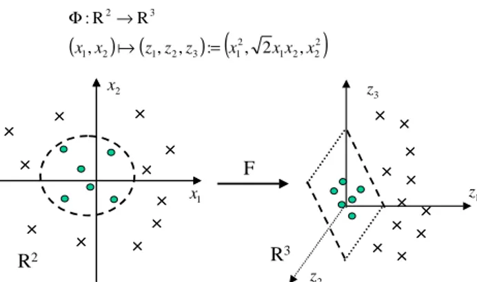
The Support Vector Machines model is the most recent proposition on neural network structures. This model is based on the statistical learning Theory. The Support Vector Machine model consists on a transformation of the input vectors X in a space of higher dimension Z through a nonlinear transformation, selected a priori. It is in this new space Z that we can build an optimal hyperplane [3]. For the particular case of pattern recognition, the SVM make a distinction of two classes by finding a decision surface constructed from certain points of the entire learning database, called Support Vectors [4].
Vapnik proposes a representation of a SVM in the form of one-hidden layer neural network whose number of cells is equal to the number of "support vectors", and not to the dimension of the space of the internal representations, as we could have supposed it initially. In this manner the number of neurons is obtained in an automatic way with the resolution of a quadratic problem. The support vectors are the input vectors xi for which equality yi((w0xi+b0)=1 holds.
Concretely, they are the closest points to the optimal hyperplane. For all the other examples, there is thus a factor
α=0 that eliminates them from the solution. We thus know that the decision function is calculated from the examples that are on the margin. In the non-linear case, it is enough to replace the scalar products (x⋅xi) by kernels k(x,xi). The
kernel functions were proposed to build nonlinear algorithms from linear algorithms by calculating the inner product not in the input space but in the feature space. Figure 1 shows this transformation.
The three most common options for the selection of the kernel function of the SVM method are the polynomial, RBF and sigmoid neural networks. The sigmoid neural network kernel function option was rejected in this work because of the difficulty of hardware implementation. Moreover in the literature the performances obtained with this kernel function are less interesting than those obtained with the two others. The results on the applications (cf. section IV) showed that, with the polynomial kernel function we obtain a solution, for different databases, with the minimum number of support vectors. In terms of generalization we observed, particularly in the first application, that the best performances were also obtained with the polynomial kernel.
III. COMPLEXITY AND PERFORMANCES
The general equation of the SVM generalization function for classification is:
( )
= ∑
(
)
+ tors SupportVec i i i k x x b y sign x f ,α α , (1) Where:yiαi=wi, are the network weights, xi, are the support vectors of the solution, b, is the threshold of the function, and k(x,xi).is the kernel function.
As we can see, the solution is the sign of the sum, which is the generalization function for two-class’s classification. In our case, the kernel function is the polynomial function of degree d: d
c
y
x
y
x
k
(
,
)
=
(
⋅
+
)
(2)The principal parameter of the polynomial kernel function is the polynomial degree. We take as a priori choice a polynomial of degree 2 (a higher degree implied the use of wider data buses in the hardware implementation).
A. Complexity
Let us suppose that the image size is tm x tm and that tb x tb
is the detection window size. tb2 is thus the number of pixels
to be processed by the window of classification. Here we consider a decision function of SVM with a polynomial kernel of degree d:
( )
[
(
)
]
+ + ⋅ =∑
tors SupportVec d i i i x x b y sign x f ,α α 1 (3) If we write wi =yiαiwe have:( )
[
(
)
]
+ + ⋅ =∑
tors SupportVec d i i x x b w sign x f ,α 1 (4)To make the classification of all the windows of pixels of one 512x512 image, with no sweeping, and a 8x8 detection window, we have 64x64 (tm/tb)2 windows to process. Each window (or input vector) requires tb2 operations (operation =
multiplication + addition) for the scalar product of the kernel function (x•xi) and d multiplications for power operation,
which we also consider as one operation for simplicity, we have then:
1
2+ +
d
tb operations per support vector.
(
) (
)
(
2)
2 2 1 2 1 3 2 1 2 1 3 2 , 2 , : , , , R R : x x x x z z z x x = → Φ a F R2 R3 2 x 3 z 1 x 2 z 1 zFig. 1. Kernel functions are used to transform the input space into feature space where the optimal hyperplane is constructed.
The additional operation is due to the multiplication between the weight wi and the result of the polynomial and
the addition of the threshold b. Let N be the number of support vectors obtained during learning, we will then have:
(
2+ +1)
× t d
N b operations per block. For (tm/tb)2 windows per image we obtain:
(
)
2 2 1 × + + × b m b t t d tN operations per image.
By making a simplification and knowing that in general
1 2>> + d tb , we thus have, 2 m t
N× operations per image. That means that the number of operations to be calculated depends on the image size and on the number of support vectors. The size of the window thus does not have a significant influence on the complexity of the algorithm. Nevertheless, this size will represent a fundamental factor during the material implementation because it will be used to dimension part of the circuit.
Now, if we use a sweeping classification window over the image, we will classify pixels several times. In this case, there will be more windows to analyze per image: (tm/p)2; where p is the number of sweeping pixels (can also be seen as the classification resolution). For example for p=2, i.e. we move in the image with a step of 2 pixels at a time, horizontally and vertically. We then get:
(
)
2 2 2 2 1 m b m b N t p t p t d t N × × ≈ × + +× operations per image.
In the case of a 8x8 detection window and a sweeping step of 2 pixels, we will make 16 times more calculations than without sweeping. The advantage of using sweeping would be to increase the image sampling and to classify several times each pixel or window of pixels and thus to obtain a more robust decision, and also to increase at the same time the localization precision. The complexity for a traditional image processing algorithm like filtering by a convolution direct method, depends on the size of the convolution mask (MxM for example) and on the size of the processed image, therefore the number of operations is given by:
2 2
m t
M × operations by image.
Table 1 summarizes the algorithm complexity analysis. Applying a convolution mask to an image is less expensive in computing requirements than the other algorithms if the size of the mask M is higher than 9. Nevertheless, applying the convolution mask is only the first step to solve the problem of object detection and localization.
In general, if we use a classical method for object recognition, the complexity of the system will be the
addition of the complexity of each subsystem. It will also depend on different parameters of the processed image, for example: edges density, line density and the ratio between the object and the image size. For the SVM method, the complexity depends only on a priori chosen parameters.
B. Performances
We carried out some measurements of execution times. As we have shown, the number of operations and the computing time increases proportionally to the number of support vectors. We thus find the main disadvantage of the Support Vector Machine method: the number of support vectors. This number is automatically obtained during learning; we cannot control this parameter without modifying the generalization performances.
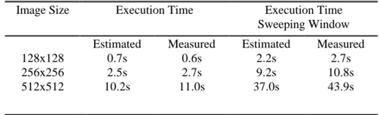
These measurements of execution times were made on a Sun Microsystems ultra 5 workstation.
For the estimation of the computing time, we obtained that a multiplication-addition operation is executed in 470ns. We obtained this time from a program carrying out a loop of 106 iterations. In this loop as in the software implementation of the function of generalization of the SVM we used the mathematical function pow(). Estimated times are slightly larger than measured times. This is due to the use of the indices in the estimation program. Table II shows some results.
C. Learning Performances
The learning algorithm uses a decomposition method to increase the learning performance and to reduce the necessary resources of the machine on which we execute the learning algorithm, in particular memory resources. This algorithm calls the generalization function and supposes that we can define a working set (vectors or examples) B such as |B|≤L (L is equal to the number of examples or vectors of all
the learning database, and |B| the number of B elements). This set is sufficiently large to contain all the support vectors (αi>0), but sufficiently small so that the hardware platform
(PC, workstation, etc.) can handle them and optimize them by using the quadratic optimization algorithm.
The decomposition technique can be written in the following manner:
1. Choose in a random way |B| points of the database. 2. Resolve the sub-problem defined by the elements in B. 3. Repeat the 3 steps while there exist a j ∈ N, such as
g(xj).yj<1 (which corresponds to a bad classification),
where
( )
∑
(
)
=+
=
l p p j p p jy
K
x
x
b
x
g
1,
α
(5) TABLE ISUMMARY OF ALGORITHM COMPLEXITY
Algorithm Number of operations
SVM 2 m
t
N
×
SVM Sweeping window 2 2 m b t N p t × × Convolution 2 2 mt
M
×
TABLE IIEXECUTION TIMES FOR DIFERENT IMAGE SIZES. 16X16 WINDOW SIZE, 88
SUPPORT VECTORS
Image Size Execution Time Execution Time
Sweeping Window
Estimated Measured Estimated Measured
128x128 0.7s 0.6s 2.2s 2.7s
256x256 2.5s 2.7s 9.2s 10.8s
The algorithm, at each iteration, improves the objective (optimization) function and is not, in this sense, recursive. Since the objective function is limited, the algorithm converges towards the optimal solution in a finite number of iteration [5].
The function g(xj) is in fact the SVM generalization
function. And for instance, if we are able to reduce of two orders of magnitude the execution time of this part of the algorithm will improve the learning performances and we could have a real-time learning algorithm.
We can observe the experimental results of the execution time of the learning algorithm according to the size of the working subset B in Fig. 2. The learning process is clearly accelerated with this decomposition method. According to these simulation results, for a real-time learning system and for subsets of average sizes, it would be necessary to increase the performances of the execution of the quadratic optimization algorithm. We can also observe in Fig. 2 that the execution time of the SVM generalization function is practically constant, that is approximately 100 seconds. This is because the calculation of g(xj) is made for all j of the
database and thus does not depend on B. For B lower than 200, the execution time of the learning algorithm is practically dominated by the generalization subroutine.
As we also can see, the software execution times are prohibited for real-time applications. This is the reason of the hardware implementation. We are now presenting some of the results on one of the three tested applications and then we are going to detail the architecture at different levels. IV. APPLICATIONS
The excellent performances of the SVM for classification problems were very attractive from the beginning of their proposal. This is true especially if we consider that the method can be applied directly on pixel values, and it does not need to take into account any other a priori problem knowledge and “a permutation of the images by a fixed transformation does not modify the SVM classifier performances” [6].
The performance analysis of the SVM methods on databases used as «benchmarks» by the scientific community
were already reported in literature [3][7]. Other evaluations were made on synthetic databases [8]. The principal interest of our contribution is to study this method for real-life applications (matrix bar codes detection, face detection in an automobile cockpit and the white lines detection). We have found that the SVM method makes possible to build very powerful classifiers (polynomial, RBF or perceptron).
A. Detection and localization of matrix barcodes.
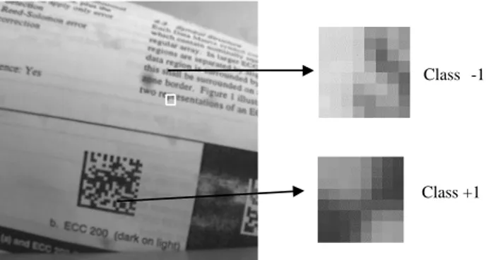
Bar codes are essential as product identification, either during manufacturing or marketing. The market requirements made very important the fine resolution of questions like reading robustness under very diverse conditions. The effectiveness of barcodes is so interesting that the vendors would wish to be able to put more information on them. A linear bar code, for example EAN13 code, can code 11 characters (numerical 0-9), this code is generally used like reference for a product index. The aim of matrix barcodes is to be able to code more than 2000 alphanumeric characters, and to thus be able to have product information like its price and its principal features. That supposes to evolve from a one-dimensional code to a two-dimensional code. And two-two-dimensional codes suppose image processing and recognition.
This study was made with the collaboration of INTERMEC Company. INTERMEC provided a base of 78 images with different types of matrix barcodes and various image sizes. The study was based on the DATAMATRIX code. We have also shown results of generalization on other types of codes. Each pixel value is coded on eight bits, i.e. in 256-gray levels from 0 to 255.
The images show different scenarios like projective deformations, different image backgrounds, different scales, etc. For this application we find the object by segmenting the image and not by finding directly the whole object, i.e. we benefit from the texture regularity of matrix bar codes to locate them. In [9], the author proposes, for the localization and the automatic reading of matrix bar codes, to use the texture to validate the different zones found by the localization algorithm. The objective thus for this first application is to learn texture from a matrix barcode DATAMATRIX, and to make a localization of these codes in new images through image segmentation.
Databases creation is a delicate task for the methods that use supervised learning algorithms. The solution of the neural network will depend exclusively on the examples of
Fig. 2. Execution time of the learning program, the optimization and generalization subroutines of the SVM method. Obtained by using a database of 4096 examples of dimension 64.
Class +1 Class -1
the learning database. Since the SVM method is also based on learning from examples, a given "optimal" learning database provides an “optimal” solution.
In this application, we feed the learning algorithm with examples of the “positives” parts of the image (a matrix barcode), and with other textures (text, images, etc.) as “negative” examples. Two classes are thus defined (see Fig. 3): a block of pixels with the texture of the matrix barcode (class +1), and a block of pixels with a different texture (class –1). Two detection window sizes were tested: 8x8 pixels and 16x16 pixels.
We present the learning results over one database and the respective result in generalization. The first database was created from the image shown in Fig. 3. In the following table, we show learning results with a database of 4096 input vectors of dimension 64 (8x8 pixels), with 240 positive examples. The number of support vectors is indicated in Table III for different kernel functions and different values of the penalization parameter C.
We created a test database from three different images. This test database consists of 12288 examples, including 10% of positive examples. In generalization we obtained 91,8% of good classifications (positive or negative), 3,8% of not-detection (when the example is positive and the result of generalization is negative), and 4,2% of false detection (when the example is negative and the result of generalization is positive).
For a second test database with 10465 examples, including 25% positive, we had 85% of success or good classifications, 11% of not-detection and 4% of false alarm. The fact of having a relatively small percentage of false alarms compared to the number of not-detection led us to define a post-processing module based on a morphological processing for this particular application. In the images of Fig. 4, we show some qualitative results of detection, i.e., we show two examples of the output binary images.
We seek to use the best solution with a minimal number of support vectors. These results were obtained with the second-degree polynomial kernel function solution and with the penalization parameter C=200. The first image shows the result of the test since the learning database was created using this image. More detailed information can be found in [10].
V. PARALLEL NEURAL ARCHITECTURES
The regularity of image processing and neural network algorithms encourages the use of parallel VLSI circuits. Parallelism is an intrinsic notion of the neural networks, which are regarded as massively parallel systems [13]. In spite of the enormous computing power obtained with new sequential processors, it is possible that these types of processors are not sufficient for real time applications. There are some solutions with neural networks, which use classical sequential processors. For example, the optical character recognition algorithms (OCR), whose performances are acceptable for applications that do not require a real time operation.
A significant number of analog implementations were proposed, exploiting the biological origin of neural networks, which illustrates the use of individual simple cells but interconnected by a network and functioning in a massively parallel way. In the particular case of the integrated artificial retinas, the use of analog circuits is a choice impossible to avoid. Because we want to be able to bring processing as near as possible to the photosensitive circuit and to be able to manage the interconnections more easily (each pixel interacts with its closer neighbors) [14][15].
Many neural implementations in numerical integrated circuits have been proposed. The finality of these circuits is to be used within traditional workstations like neural coprocessors, in acquisition and signal processing cards, in order to make more intelligent sensors, or to be used as specialized parallel-processing machines. They are generally dedicated to a single neural model, and all do not propose a learning integrated procedure [16]. There are thus several types of neural systems:
Application Specific Architecture implement a model, a topology and a set of weights, mostly by analog means. Problem Specific Architecture implement a model and a given topology; the weights of the network are programmable. The learning is done most of the time off-line.
With Algorithm Specific Architectures, the model is selected a priori. Topology can be modified, and the learning is carried out by the system itself.
Neural Processor Architectures are also called multi-model
TABLE III
NUMBER OF SUPPORT VECTORS FOUND DURING LEARNING FOR DIFFERENT KERNELS AND VALUES OF PARAMETER C
Kernel Degree Value of C
10 200 500 5000 Linear 491 547 620 1320 Polynomial 2 316 310 321 320 Polynomial 3 333 343 325 311 Polynomial 4 341 310 311 311 RBF 2 385 333 312 304
Fig. 4. Image segmentation results using the SVM as detection system. The window size is 8x8 pixels. A post-processing algorithm is used in order to erase the bad classifications of the SVM.
accelerators. They are much closer to a generic processor [16][17].
VLIW Digital Signal Processors (DSP) can also be used to implement neural networks, but they are more generic processors. Many DSP chips are available, like EQUATOR MAP-CA BSP, NEC SPXK5 or Analog TigerSHARC that include a small degree of parallelism. Some are built around a large parallel processor structure (VLIW) linked to a scalar RISC processor, in a single core structure. For example, the SIROYAN SRA328 [19], which is much more a real multiprocessor. The CHIPWRIGHTS CWv8 processor core [20] is much more a SIMD processor. The RC MODULE NeuroMatrix NM6403 core [18], which is a real full vector/matrix parallel processor provides scalable performances and a programmable operand width of 1 to 64 bits. This flexibility allows designers to trade precision for performance to suit their applications. The NM6403 processor includes a 32/64-bit RISC processor and a 1- to 64-bit vector coprocessor that supports vector operations with elements of variable bit lengths. The vector coprocessor, with SIMD (single-instruction-multiple-data) architecture, works on packed integer-data comprising 64-bit blocks in the form of variable 1- to 64-bit words. The device is limited to vector-matrix or matrix-matrix multiplications. The Vector coprocessor’s core looks like an array of multipliers comprising cells that include a 1-bit memory (flip-flop) surrounded by several logical elements. Designers can combine the cells into several macrocells with two 64-bit programmable registers. These registers define the borders between rows and columns with macrocells. Each macrocell performs the multiplication on variable-input words using preloaded coefficients and accumulates the result from the macrocells in the column above it. The columns simultaneously calculate the results in one processor cycle. For 8-bit data and coefficients, the vector coprocessor performs 24 MAC (multiply-accumulate) operations with 21-bit results in one processor cycle. The number of MAC operations depends on the length and number of words packed into a 64-bit block. The engine’s configuration can change dynamically during calculations. An application can start with maximum precision and minimum performance and dynamically increase performance by reducing the data-word lengths.
VI. THE OBJECT RECOGNITION SYSTEM
If we take the classical and simplified architecture of an object recognition system, we have the following modules: image sensor, detection, localization and diagnosis. For our implementation we propose a PC-based recognition system, and use a standard camera as image sensor. Therefore, it is the detection module that we will hardware-implement using the SVM as its core. In order to be able to integrate the detection module in the PC-based system we will use the PCI interface.
VII. THE SOCPLATFORM ARCHITECTURE
A particular SoC category concerns the SoC platforms [21], an emerging technology which main purpose is to provide a reusable silicon platform for many applications,
either for several versions of a single application or even for several different applications in the same field. This is due to the growing design and fabrication costs of ASICs, which thus impose large amounts of chips. The only solution is to have more general reusable chips. The Xilinx VirtexPro II can be considered as a general purpose SoC platform, which associates dedicated blocks such as PowerPC processors, RAM and multipliers, and a classic FPGA part that can be dynamically reconfigured.
The platform we are proposing here is dedicated to fixed-point vector/matrix operations, which are the basic operations of many signal and image processing functions. We have concentrated our effort on neural network applications.
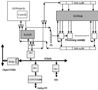
Figure 5 depicts the general architecture of our proposed SoC platform. This platform is built around a RISC 32-bit processor linked to a parallel vector coprocessor. Both are connected to a Network-on-Chip (NoC) [22] that controls communications between the different parts of the system. Here the NoC is a PCI-X On Chip Bus (OCB) version. We have simplified the LEON-2 SPARC processor (1) in order to communicate directly from its cache memory (2) to the dual-ported RAM (3) used to store LEON-2’s binary code and data. A second data RAM (4) is accessible in the memory address space of both the LEON-2 processor and the external I/O subsystem (5), which is here a simple On Chip Bus with its wrappers (light-gray boxes). This dual-ported RAM is the storage unit of the CP CoProcessing vector/matrix unit (6) which performs ALU/MAC operations loops on vector/matrix fixed-point data from the RAM, according to the instruction register (7) which provides the configuration of the processing units. This register is detailed in figure 6. The ALU allows any kind of operations to be executed, leading to a richer instruction set than the simple MAC operations of most similar approaches such as the NeuroMatrix chip [18].
This is a double register operating in ping-pong mode. This register is reconfigured for each new matrix operation. The configuration that is provided to the vector processing
LEON-light (1) Cache(2) RAM(3) RAM(4) Shift reg(9) Shift reg(8) Bridge CAN/CNA(10) FIFO Analog I/O Digital I/O(12) OCB(5) Processing units(6) (7) (11) LEON-light (1) Cache(2) RAM(3) RAM(4) Shift reg(9) Shift reg(8) Bridge CAN/CNA(10) FIFO FIFO FIFO FI FO Analog I/O Digital I/O(12) OCB(5) Processing units(6) (7) (11)
unit is, the size, step and addresses of the loops, the precision of data and the operations performed with or without accumulation.
Here it is an example of matrix/vector operation with accumulation:
For (J=start2; J<size2; J+=step2) { For (I=start1; I<size1; I+=step1) {
Res[J] = Res[J] op2 (RAM1[I] op1 RAM2[I]); } }
Fig. 7. General parallel loop pattern
The (8) and (9) registers are used to shift input and output data in and out of the vector RAM. These registers can also broadcast input and output data in the case of vector/matrix operations to be treated as matrix/matrix operations.
The multi-precision unit is presented on figure 8. This is a version with only two different input precisions (8-bit and 16-bit), in order to simplify the presentation. The first OP1 operator is either a 8x8 multiply or a 8-bit ALU. The 16-bit result can be accumulated with the 32-bit OP2 operator. The two 8-bit multiply operators (OP1) can also be combined to perform a 16-bit multiply in two clock cycles, using the accumulation operator (OP2) to perform the two additions. A 16-bit MAC is thus performed in four clock cycles, that is two for the four multiply operations, one for the last addition of the 16-bit multiply results and one for the final accumulation. The accumulation is pipelined with the preceding operation, which is thus treated every clock cycle for an 8-bit MAC. Every 3 cycles for a 16-bit MAC and every 5 cycles for a 32-bit MAC, that is every N+2 cycles with N the number of bytes of data precision. The main limitation of our proposed architecture is the vector data precision which must be a multiple of 8 bits, which however is often the case in image processing. The counterpart is the lower complexity of the logic which lead to higher clock frequencies, compared to the Neuromatrix solution which is a 1-bit multiple with a lower clock frequency.
The last part of the system is the I/O subsystem, which has to feed the processor with data. The OCB is used as the central communication subsystem between the
processor/coprocessor and the external analog (10) and digital (12) ports. Other components can also be integrated on the OCB (11), like other processor/coprocessor couples in order to build a complex system. A single large coprocessor with many processing units would be difficult to manage due to the limited available data and instruction parallelism as well as the long distances between units which would affect their communications and the clock frequency. Here it is figure 9 an example of configuration obtained from the original and adapted C SVM source codes of figure 10 and 11. The CoProcessor here executes only the two internal loops. These internal loops are packed in a function.
The Acquisition() function start a DMA with the CoProcessor RAM, and the Sync() function waits the end of the CoProcessor treatment and switch the configuration register and RAM banks to prepare the next treatment. The ALU X ALU ALU X ALU OP1 : OP2 : ALU X ALU ALU X ALU OP1 : OP2 :
Fig. 8. Multi-precision Processing Unit
@start1 Size1@start2 Size2 @Dest. Precision OP1OP2BroadAccum.
Fig. 6. Configuration Instruction Register
int CP_Recognition(int nb_sensors, int nb_supports) { int k,j;
for(j=0; j<nb_supports; j++) for(k=0; k<nb_sensors, k++)
oo[j] += support_vectors[nb_sensors*j+k]*sample[k]; }
Support_vector nb_supports sample nb_sensors oo 8 + x no acc.
Fig. 9. CP_Recognition() function and equivalent configuration.
/** RECONNAISSANCE ******************************************************/ /**************************************************************************/ void
recognition(sample, nb_samples, nb_sensors, std, support_vectors, support_weights, support_threshold, nb_supports, kernel, classe, gausse, var_thresh)
int *sample; int nb_samples; int nb_sensors; float std; int *support_vectors; float *support_weights; float support_threshold; int nb_supports; char *kernel; int *classe; double var_thresh;
{
double out; double oo; int i,j,k; struct timeb debut,final; FILE *fichier; for(i=0; i<nb_samples; i++){
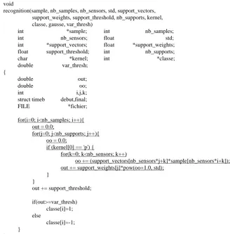
out = 0.0; for(j=0; j<nb_supports; j++){ oo = 0.0; if (kernel[0] == 'p') { for(k=0; k<nb_sensors; k++) oo += (support_vectors[nb_sensors*j+k]*sample[nb_sensors*i+k]); out += support_weights[j]*pow(oo+1.0, std); } } out += support_threshold; if(out>=var_thresh) classe[i]=1; else classe[i]=-1; } }
Fig. 10. Original C-code of the SVM generalization function. The part of the code that is executed on the co-processor is underlined
for(i=0; i<nb_samples; i++) { out =0; for (j=0;j<nb_supports;j++) oo[j]=0;
CP_Recognition(nb_sensors,nb_supports); // non blocking
Acquisition(sample); // non blocking
Sync(); // blocking
for (j=0; j<nb_supports;j++) out+=support_weights[j]*pow(oo[j]+1); out+=support_threshold;
if (out>=var_thread) classe[i]=1; else classe[i]=0; }
reconfiguration is performed by program (LEON-2 C code), with dynamically constructed vector instructions (configurations). We have developed a preprocessing C parser which analyzes CP_name() functions, which have to comply with the pattern of figure 7. This preprocessing links the parameters of the loops to the dedicated C library function which will dynamically, that is at run-time, fill the fields of a configuration instruction register which will then be launched to the CP core (CoProcessor). Those configurations represent the nature of the processing, that is the SVM processing. This vector coprocessor architecture is a good compromise between a fully hardwired solution and a fully programmable general-purpose solution. A first small C library has been designed for our SVM experiments. This approach can be compared to the Neuromatrix one [18], which is the only comparable product on the market. Their approach is based on a static compile-time generation of configurations, which is most of the time sufficient and as easy to program as our solution, but dynamicity becomes more and more important. This is particularly important when the reconfiguration needs to be dependent of the previous results of a processing, in a non-predictable way. The heart of our learning procedure is based on the
classification procedure, which is evaluated here. The dynamic nature of the parameters is used here in the learning phase, which calculates the interesting support vectors, their number, and their size according to the quality of the classification. These results can be re-injected in the classifier treatment in order to size the final classifier parameters. Thus, this non-supervised approach leads to an automatic parameterization of the classification treatment. This SVM solution, which is optimal in terms of database classification, can thus be used as an automatic solution to many treatments, which can be adapted and solved by means of classification. This kind of approach is only possible if a large size hardware is available, that is in a near future.
This application could be also implemented on the Neuromatrix chip, but with lower execution time (or higher
costs). The scalability of the application, which is linear for matrix operations can be dealt in two ways. First, when the size of the loops is higher than the size of the CoProcessor, a second internal level of loop is performed in the coprocessor structure by means of RAM address management, that is with a circular data mapping in the RAM array. Second, when the data size is higher than the RAM size, the treatment has to be divided in smaller parts manually at compile-time, either on the same CoProcessor by serialization, or on several different CoProcessors linked together through the Network on Chip, that is here the PCI-X On Chip Bus. A future data cache RAM array architecture is under study in order to mask this limitation to the programmer. Both solutions lead to performances or cost impact due to serialization of operations.
VIII. RESULTS
A. The choice on SVM parameters.
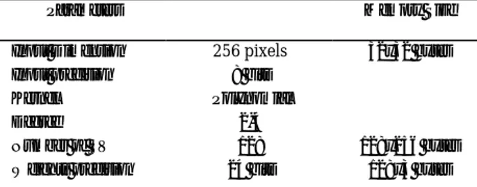
The retained kernel function of the SVM machine is the polynomial. Because of the obtained performances and also because its hardware implementation is relatively easier. The principal parameter of the polynomial kernel function is the degree of the polynomial. Although it is possible to make an implementation with a variable polynomial degree, we took as basic choice a polynomial of degree 2 (a higher degree would impose the use of wider data buses). Considering that our principal application is the matrix bar codes detection, we took 16x16 pixels as the detection window size for the hardware implementation. This size is not important to the application level. Table VI summarizes the behavioral specification of the SVM classifier.
B. The choice of the hardware parameters.
We have chosen to implement the SVM classifier on a SoC platform in order to exploit the parallel nature of the SVM algorithm. The active logical blocks and the interconnection buses normally consume the surface of silicon of an ASIC or FPGA circuit. For a few years, interconnection busses became the main consumers of silicon surface, due to the complexity of algorithms and circuits.
Input Data: the values of pixels are coded in 256-gray levels, therefore all memories with pixel values will be used as a multiple of 8 bits. So each element of the support vectors will correspond to an 8-bit value.
Weight Data: It is the only data whose size is not defined by the specification. It is significant to define its size precisely, in order not to modify the recognition performances significantly. Although the values in the software implementation are float values, in the hardware
TABLE VI
SVM CORE BEHAVIORAL SPECIFICATION
Kernel Function Polynomial
Degree of the Kernel function 2/3/4
Number of support vectors 128
Input Dimension 64 or 256
TABLE IV
HARDWARE PARAMETERS SUMMARY
Parameters Memory Size
Input Dimension 256 pixels 32x32 bytes
Input precision 8 bits
Kernel Polynomial
Degree 2-4
Number of SV 128 128x256 bytes
Weights precision 24 bits 128x3 bytes
TABLE V
VHDL XC2V3000 SYNTHESIS SUMMARY
blocs Size frequency
32-bit LEON2-light 14 % 50 MHz
64-bit OCB interface 6 % 133 MHz
64 8-bit coprocessors 60 % 166 MHz
LEON2 RAM 32 Kbytes
-implementation we use fixed-point to avoid the use of the floating-point operators. The results of weights precision analysis were obtained from the same database used for testing the SVM algorithm. We vary the precision (number of bits) of the weights and we obtain the percentage of good detection and of bad classifications, the rest corresponding to false alarms.
In opposition to the results obtained by A. Bermak [11] and those shown in literature [12] where the average is 8 bits, the necessary precision to have the same success rate that we obtained by software is near 16 bits. It is a relatively high precision compared to the implementations shown in literature. Different factors can explain this result: for off-line learning we have in general a more significant precision [12]. Afterwards, the weights obtained during this learning process must be approximated to their hardware precision. In our case, the learning precision is maximal. Other models have fewer neurons than the SVM: this requires less precision for a hardware implementation. And finally, let us recall that the hyperplane of separation in the case of the SVM is in a dimension, which is much higher than the input dimension, and that the solution is built up using the support vectors. The 32 bits of the processor outputs are sufficient to provide the result to the generalization function, which operates on the data weights. The LEON processor performs this last function, which is limited in complexity, sequentially and in pipeline with the matrix product.
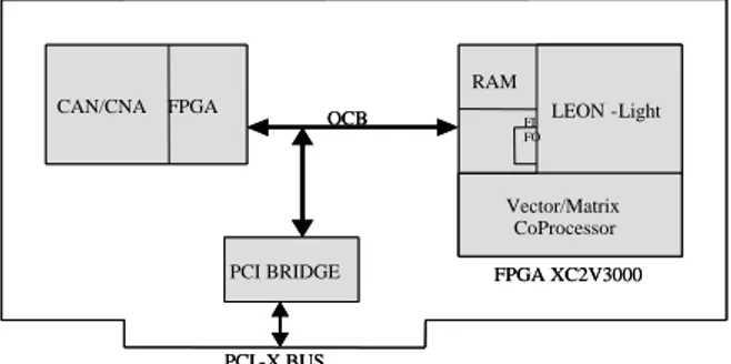
C. Prototyping Platform.
We have designed a general rapid prototyping platform dedicated to SoC emulation. The central board connects a CAN/CNA module with a Xilinx XC2V3000 FPGA and a PCI-X controller. This general-purpose board is presented on figure 12. A more complex system can be built with several boards on the PCI-X bus, which corresponds, to the OCB of our final SoC. We have implemented and validated the presented application on this single board. The synthesis results obtained are presented on table V. The vector coprocessor RAM is organized in two 1Kbytes RAM per processing unit. The peak performances of 10 Giga MAC/sec have been reached with this application. As a comparison, the number of gates of our chip is nearly the double compared to the Neuromatrix core. Also, the main vector/matrix product consists of 256*88 8-bit multiplies, that is 256*88/64=352 clock cycles compared to the
16*88=1408 clock cycles with the evaluated Neuromatrix chip. We have thus obtained an efficient solution, easy to program. A large SoC will be studied on CMOS 0.13µm technology ASIC in order to obtain real-time execution with more important applications.
IX. CONCLUSION
Platform Based Design (PBD) is the best-validated industrial approach for achieving high reuse in SoC design, and incurs the lowest risk in derivative creation via user programmability. Although these platforms already exist in some application domains, their design process is largely ad hoc. Furthermore, despite high development costs, such platforms tend to be difficult to program, and very little software support is available. Our proposition attempts to fill this gap. Our approach is to provide a general-purpose neural network application customized by a learning phase instead of explicit programming which avoid tedious designing effort. Such a solution is only possible with large hardware platforms. We have proposed in this paper a sizeable SoC platform dedicated to regular image and signal processing involving matrix operations. We have illustrated its implementation capabilities with the SVM neural network application, which performs object recognition of any kind (image or signal). A user-friendly interface is under construction. Also a future ASIC SoC implementation will demonstrate the feasibility of our approach on realistic objects recognition. With such a system, it is possible to obtain an automatic object recognition/classification based on a learning phase, which automatically configures the recognition engine, and then obtain a real-time toolbox for any object classification.
ACKNOWLEDGMENT
We thank INTERMEC for the image databases used to show the performances of the SVM method for a real application. Roberto Reyna thanks the Mexican Research Council for its financial support through the studentship 111030.
REFERENCES
[1] C. M. Bishop. “Neural Networks for Pattern Recognition”. Oxford University Press. 1995.
[2] B. E. Boser, I. M. Guyon, and V. N. Vapnik. “A learning algorithm for optimal margin classifier,” Proceedings of the 5th ACM Workshop
on Computational Learning Theory, 1992, pp. 144-152.
[3] V. N. Vapnik. “Statistical. Learning Theory”. A Wiley-Interscience Publication. 1998.
[4] C. Burges. “A tutorial on Support Vector Machines for Pattern Recognition”. Kluwer Academic Publishers.
[5] E. Osuna and F. Girosi. “Reducing the run-time Complexity of Support Vector Machines”. International Conference on Pattern Recognition, 1998.
[6] Y. LeCun, L.D. Jackel et al. “Comparison of learning algorithms for handwritten digit recognition”. In F. Fogelman-Soulié and P. Gallinari, editors, Proceedings ICANN’95 – International Conference on Artificial Neural Networks, volume II, pp. 53-60, Nanterre, France, 1995.
[7] B. Schölkopf. Support Vector Learning”. Ph.D. dissertation. Technical University Berlin. September 1997.
CAN/CNA FPGA PCI BRIDGE LEON -Light Vector/Matrix CoProcessor FPGA XC2V3000 OCB PCI -X BUS RAM FI FO CAN/CNA FPGA PCI BRIDGE LEON -Light Vector/Matrix CoProcessor FPGA XC2V3000 OCB PCI -X BUS RAM FI FO
[8] V.L. Brailovsky, O. Barzilay, R. Shahave. “On global, local, mixed and neighborhood kernels for support vector machines”. Pattern Recognition Letters 20 (1999), pp. 1183-1190.
[9] B Marcel. “Study on the automatic reading of two-dimensional codes by image processing”. Ph.D. dissertation. Institut National Polytechnique of Toulouse. December 1997.
[10] Roberto Reyna-Rojas, M. Cattoen, D. Esteve, N. Hernandez. “Segmenting images with support vector machines”. Proceedings of the 2000 IEEE International Conference on Image Processing (ICIP'2000), Vancouver (Canada), 10-13 Septembre 2000, Vol.I, pp.820-823
[11] A. Bermak. Sysneuro : Un circuit Systolique Neural multipécision pour des tâches de classification. Ph. D. Thesis dissertation. Université Paul Sabatier de Toulouse. LAAS report number 98395. September 1998.
[12] P. Moerland and E Fiesler. Neural Network Adaptations to Hardware Implementations. IDIAP Research report IDIAP-RR 97-17. Handbook of Neural Computation, E1.2:1-13. Institute of Physics Publishing and Oxford University Publishing. January 1997. [13] A. Jain, R. Duin, J Mao. Statistical Pattern Recognition: In Review.
IEEE Transactions one Pattern Analysis and Machine Intelligence. 22(1). Pp. 4-37. 2000.
[14] C. Koch and H. Li. Vision Chips: Implementing Vision Algorithms with Analog VLSI Circuits. Los Alamitos: IEEE Computer Sciences Press, 1994.
[15] L.O. Chua and L. Yang. Cellular Neural Networks: Applications. IEEE Transactions on Circuits and Systems, Vol. 35, No. 10, pp. 1273-1290. October 1988.
[16] M. F. Emirian. Study and design of a parallel machine multi-models for the neural networks. Ph.D. Thesis. Institut National Polytechnique of Toulouse. December 1996.
[17] M. Viredaz. Design and Analysis of a Systolic Array for Neural Computation. Ph.D. Thesis. Ecole Polytechnique Fédérale de Lausanne. 1994.
[18] Research Center MODULE. VLIW/SIMD NeuroMatrix Core. Moscow, Russia.
[19] Peter Clark. Siroyan implements clustered DSP architecture. EE TIMES, October 15, 2001.
[20] Mark Long. ChipWrights Intros New Visual Signal Processor. ECN magazine, October 2003.
[21] A. Sangiovanni-Vincentelli, G. Martin. "Platform-Based Design and Software Design Methodology for Embedded Systems", IEEE Design and Test of Computers, November, 2001
[22] L. Benini, G. De Micheli, “Networks on Chip: A New SoC
Paradigm”, IEEE Computer, 2002.
Roberto Reyna-Rojas (S’2000, M’2004) was born in Tehuantepec, Mexico, in 1972. He received the Electronics Eng. degree from the Universidad Autonoma Metropolitana, in Mexico City, in 1994 and the Computer Science Eng. degree from ENSEEIHT Toulouse, France in 1997. He obtained the Ph.D. degree from the National Institute of Applied Sciences, Toulouse, France in 2002. He is actually working for the French Space Agency CNES in VLSI circuits Failure Analysis, and particularly failures provoked by ESD events. Her research interests are in the area of VLSI design and reliability, development of integrated neural networks and specific signal processing architectures. Email: [email protected].
Dominique Houzet received the MS in computer sciences in 1989 from Paul Sabatier University, Toulouse, France and the Ph.D. degree and HDR degree in computer architecture in 1992 and 1999 both from INPT-ENSEEIHT, Toulouse, France. He worked at IRIT Laboratory and ENSEEIHT engineer school from 1992 to 2002 as assistant professor and also as digital design consultant with SME. He is an associate professor with the Department of Telecom, at the National Institute of Applied Sciences, and IETR Laboratory, Rennes, France, since 2002. He has published a number of research papers in the area of parallel computer architecture and SoC design and a book on VHDL principles. His research interests include co-design and SoC design methodologies applied to image processing and radiocommunications. He is a member of IEEE computer society. Contact him at [email protected].
Daniela Dragomirescu (S’97, M’2001) was born in Bucharest, Romania, in 1972. She received the Electronics Eng. Degree from Bucharest Polytechnic University, Romania, in 1996 and her Ph.D. degree from the National Institute of Applied Sciences, Toulouse, France. She has been an Associate Professor at Toulouse National Institute of Applied Sciences (INSA) since October 2001 and a researcher at System Analysis and Architecture Laboratory from French National Center for Scientific Research (LAAS-CNRS). Her research interests are in the area of systems on chip and hardware architectures for signal processing. Email: [email protected].
Florent Carlier received the Ph.D. degree from the National Institute of Applied Sciences, Rennes, France, in 2003, where he specialized in neural network for communication systems. He has been IEEE Student Member. He began an academic career in 2004, as Lecturer in Numerical Electronics and member of the Department of Informatics (LIUM) from the University of Maine, Le Mans, France. His research interests include computer architecture, digital systems, protocol design and computer programming. Contact him at [email protected].
Salim Ouadjaout received an MS in computer science from National Institute of Computers (INI) of Algerier, Algeria, in 2000, and an MS from INP-ENSEEIHT in Toulouse, France, in 2001. He is a Ph.D. candidate in electrical and computer engineering at Institute of Electronics and Telecommunication of Rennes, France. He is also working as research engineer at M3Systems Inc. He has been ACM Student Member. His research interests include Design Methodology, interface synthesis and micronetworks for SoC. Contact him at [email protected].