UNIVERSITÉ DE MONTRÉAL
IMPACTS OF BUILDING SAMPLING PROTOCOL, SERVICE LINE CHARACTERISTICS, AND SUPPLY WATER QUALITY ON DISSOLVED AND
PARTICULATE LEAD AND COPPER IN DRINKING WATER
EVELYNE DORÉ
DÉPARTEMENT DES GÉNIES CIVIL, GÉOLOGIQUE ET DES MINES ÉCOLE POLYTECHNIQUE DE MONTRÉAL
THÈSE PRÉSENTÉE EN VUE DE L’OBTENTION DU DIPLÔME DE PHILOSOPHIAE DOCTOR
(GÉNIE CIVIL) AOÛT 2018
UNIVERSITÉ DE MONTRÉAL
ÉCOLE POLYTECHNIQUE DE MONTRÉAL
Cette thèse intitulée :
IMPACTS OF BUILDING SAMPLING PROTOCOL, SERVICE LINE CHARACTERISTICS, AND SUPPLY WATER QUALITY ON DISSOLVED AND
PARTICULATE LEAD AND COPPER IN DRINKING WATER
présentée par : DORÉ Evelyne
en vue de l’obtention du diplôme de : Philosophiae Doctor a été dûment acceptée par le jury d’examen constitué de :
M. COMEAU Yves, Ph. D., président
Mme PRÉVOST Michèle, Ph. D., membre et directrice de recherche M. TOBIASON John E., Ph. D., membre
DEDICATION
To my mom and dad, who taught us that there are no limits to what we can achieve
My friends, love is better than anger. Hope is better than fear. Optimism is better than despair. So let us be loving, hopeful and optimistic. And we'll change the world. - Jack Layton
ACKNOWLEDGEMENTS
First, I would like to thank my advisor, Dr Michèle Prévost. Thanks for offering me this Ph. D. project and welcoming me in your team. Thanks for being a role model and such an inspiration to us. I really loved how excited you would be when I’d bring new data during our meetings, which sometimes looked like marathons. I truly enjoyed all those hours spent discussing results, their implications, and the multiple iterations we made of flow charts and the gigantic tables we glued to your bookshelf. Thanks for always being so energetic, supportive and for really caring. I was really touched to be with you, in Cincinnati, when you learned you received the AWWA’s AP Black Award. Thank you for everything and for teaching me so much, and not just scientifically. I would also like to thank Michael Schock, whom I met at the early stages of my project. Even if you were not my co-advisor, you surely felt like one at times and tremendously helped me. Thanks for teaching me so much during those years, despite the stupid questions we asked (now I realize). Thanks for welcoming us multiple times in your lab in Cincinnati and for all those discussions, which were not always related to work, that we had with Michèle and you around a beer. I’m lucky to have had the chance to work with such an amazing researcher.
At the beginning of the Ph. D., I had the opportunity to be part of “the lead team”. Thanks Clément for trusting me with your “baby”, the lead pilot and for teaching me a lot about service lines. Thanks Elise for all the help writing papers (and re-writing them!) and for the help with the large building sampling, and re-sampling!! And for seeing that we had done enough we the pilot and it was about time to pull the plug. Thank you Shokoufeh for everything, from finding every little mistake in presentations and papers with your sharp eye to general discussions on lead.
Through the different publications and conferences, I have had the opportunity to work with several co-authors, whom I would like to thank. I would also thank the members of the examination committee, Dr Yves Comeau, Dr Darren A. Lytle and Dr John E. Tobiason. I would also like to thank Dr Marc Edwards for the advices at the beginning of my Ph. D.
I would like to thank the Chair staff. You have been there throughout my project, you’ve encouraged me, answered all my questions and always made sure things were running smoothly. You make the magic happen. Yves, thank you for everything; for building and fixing this amazing pilot, which we happily destroyed at the end, for all those hours of sampling, including all your songs and jokes, and for always having a solution to my problems in the lab. With Mireille, you
have taken care of my baby pilot when I could not be there and I really appreciate it. Thank you, Mireille, for always being there when I needed help and for all the advice you gave me. Thank you, Jacinthe, for all the DOC analysis. Thank you, Jacinthe and Julie for the help with all the purchases I had to do, giving great advice for lab work and life in general. Thank you, Mélanie for taking care of all my samples from large buildings for the HPC. Thank you, Denis for the analysis as well and for the TA position you offered me. Thank you, Laura, who is always there to help find Michèle, for EndNote and for anything we could possibly need. I would also like to extend my thanks to Manon Latour for the help will all the administrative work and to France Boisclair.
Of course, all of this work with Mike Schock would not have been possible without Dr. Michael K. DeSantis. Thank you for taking so much time to teach me about scales. Thanks for finding every possible pipe example in your lab when we visited, from the coolest ones (purple crystals in a service line!?) to the most complicated ones, to the ones from Flint. All this work on scales would not have been possible without your help. Thanks for your patience for going through all my samples with me, I know we stared at that computer screen for way too long.
I would like to thank the staff at the City of Montréal who made the metal analysis possible: Magalie Joseph and Mylène Rémillard. Thank you, Laurent Laroche, for going through all my presentation and conference papers.
Thank you, Dr. Benoit Barbeau for all the advice during my Ph. D, for being such a good professor and for the great discussions we’ve had. Thank you, Mr. Raymond Desjardins, if it were not of you, I would have taken longer to decide to do a Ph. D, you are an inspiration when it comes to teaching and how to tell a good story. Thank you, Anouk, for giving me the project on technical writing and for all the great advice.
Thanks to the many interns I’ve had during my Ph. D., thanks for your hard work: Alexandra, Alix, Cédric, Hugo, Julie, Mai, Nada and Stéphane.
Emilie, I do not know how I could thank you enough for everything, from being the perfect roommate for conferences, to having me for dinner and board game nights with your kids, helping me with questions and for always being so supportive. You are always the best when it comes to helping me improve presentations. I’ve genuinely enjoyed working with you.
Thank you, Simoni for taking care of me when I visited Cincinnati, for coming for lunch with us, for giving thoughts and advice on papers and for becoming a friend.
Thanks to my multiple office mates over the years: Mathieu, thanks for being always so positive about everything and always finding the right thing to say, Anne-Sophie for all your shoes discussions, changing my mind with baby Alexandre and for your support all along, JB for the Belgian chocolates and Margot for always being so positive and happy. Sanaz, Kim, Fatemeh and Hadis thank you for your friendship and being there all along, I’m honoured that I can call you my friends, your friendship means a lot to me. Thank you, Celso, sadly the time you were with us was too short, but you’ll always be remembered, I miss our discussion about culture and life in general. Thank you, Amélie, Arash, Cécile, Céline, Dominique, Emile, Flavia, Giovanna, Julien, Laleh, Laura-Delly, Laurène, Laurent, Lucilla, Majdala, Marie-Laure, Maryam, Melisa, Nargess, Philippe, Noam, Valentin, Vanessa. All of you have made the long hours in the lab and life at the Chair much more enjoyable.
Also, thanks to my friends outside of school for keeping me sane, François, Ann, Megan and Geoff. Thank you, Emilie, even in Australia, you’ve been a motivation as we were both working on our Ph. D. Thanks to my lifelong friends Lori, Christine and Mylène for bringing a hint of craziness in my life, and Christine for trusting me in becoming the godmother of the sweet Ludovic.
Finally, thanks to my parents, brothers, sister and grandparents. Thanks for being there every step of the way. Thanks for not asking too often the terrible question every Ph. D. student gets: when will you finish? Thanks for being always so supportive, understanding and always being there, no matter what.
I would like to thank the NSERC and the Industrial Chair partners, the City of Montréal, Veolia Water Technologies Canada Inc., the City of Laval, the City of Repentigny, the City of Longueuil and the Canadian Water Network who made this research project possible. I would like to acknowledge the NSERC graduate scholarship.
RÉSUMÉ
Lorsque l’eau traitée circule dans un réseau de distribution, sa qualité peut se dégrader lorsqu’elle entre en contact avec des éléments de plomberie pouvant contenir du plomb, tels que des entrées de service en plomb ou encore du laiton ou des soudures au plomb. À la suite des scandales de Flint (Michigan, États-Unis) et de Washington, D.C., (États-Unis), la présence de plomb dans l’eau potable a capté l’attention du public ainsi que des chercheurs. Les inquiétudes associées à la présence de plomb dans l’eau potable sont dues au fait que ce contaminant est classé comme cancérigène et qu’il est une neurotoxine. Par ailleurs, les sources de cuivre dans les réseaux de distribution sont nombreuses. Les craintes associées à la présence de cuivre dans l’eau potable sont tout d’abord d’ordre esthétique puisqu’il tache la plomberie et les vêtements à des concentrations plus basses que celles auxquelles des effets sur la santé sont recensés.
L’objectif principal de ce projet était de déterminer la présence de plomb et de cuivre, causée par la corrosion galvanique dans les réseaux de distribution d’eau potable. Ce projet de recherche se concentre sur la présence de plomb et de cuivre dans les réseaux de distribution des écoles et des grands bâtiments ainsi que dans les entrées de service en plomb à l’échelle pilote. De manière plus détaillée, ce projet visait à : (1) quantifier l’exposition au plomb et au cuivre, par la consommation d’eau potable dans les grands bâtiments et les écoles; (2) quantifier l’efficacité de mesures de mitigations telles que l’ajout d’inhibiteur de corrosion et le rinçage avant la consommation d’eau; (3) déterminer l’impact que le type de robinet a sur les concentrations de plomb et de cuivre mesurées dans les écoles et les grands bâtiments; (4) évaluer les effets à long terme des remplacements partiels d’entrée de service en plomb sous différentes qualités d’eau, ainsi que de quantifier l’importance de la corrosion galvanique; (5) mesurer l’effet de l’ajout de chlore ainsi que du changement de dose d’orthophosphates sur les concentrations de plomb dans les entrées de service en plomb avec et sans remplacement partiel; (6) déterminer l’impact des temps de stagnation avec l’échantillonnage ainsi que les impacts de l’augmentation des vitesses d’écoulement sur les concentrations de plomb et de cuivre; (7) déterminer les conditions pour lesquelles un remplacement partiel d’entrée de service en plomb permet de diminuer les concentrations mesurées au robinet et (8) d’étudier les dépôts de corrosion présents à l’intérieur des entrées de service en plomb avec et sans remplacement partiel.
L’eau potable d’écoles et de grands bâtiments, recevant différentes qualités d'eau, avec et sans l’ajout d’inhibiteur de corrosion, a été échantillonnée. L’eau plus agressive a engendré les concentrations de plomb les plus élevées au robinet. L’ajout d’un inhibiteur de corrosion a permis de diminuer les concentrations élevées de plomb. Les résultats démontrent l’importante variation dans les concentrations de plomb et de cuivre entre les divers points d’échantillonnage à l’intérieur d’un même bâtiment. De plus, les concentrations de plomb et de cuivre mesurées variaient en fonction du temps de stagnation préalable à la prise de l’échantillon. Les concentrations de plomb et de cuivre les plus élevées ont été mesurées après une stagnation d’une nuit et les valeurs ont diminué après avoir laissé l’eau couler le point de consommation d’eau. Par contre, les résultats obtenus démontrent que les concentrations de plomb et de cuivre augmentent suite à une courte stagnation et peuvent atteindre des valeurs représentant la moitié de celles mesurées après une stagnation d’une nuit. De plus, nos résultats montrent l’importance de laisser couler l’eau, minimalement les premiers 250 mL, avant de la consommer.
Les travaux ont été réalisés à l’échelle pilote en utilisant des conduites de plomb excavées du réseau de distribution de la Ville de Montréal. L'étude pilote des concentrations de plomb et de cuivre provenant d’entrées de service en plomb avec et sans remplacement partiel a démontré que des concentrations de plomb élevées sont toujours mesurées 155 semaines après la simulation du remplacement partiel. Par ailleurs, nous avons observé que les conduites de cuivre se sont passivées suite à la simulation des remplacements partiels. Ainsi, à long terme, les concentrations de cuivre ont diminué lors des échantillonnages de suivis, prélevés après stagnation de 16 heures. Nous avons aussi démontré que le rinçage à haut débit permet de diminuer les concentrations de plomb total et particulaire provenant des conduites avec et sans remplacement partiel. Ceci implique que la présence de plomb particulaire peut être diminuée par des rinçages à haut débit.
Suite à l’ajout de l’effet de la corrosion galvanique par la simulation des remplacements partiels, différents inhibiteurs de corrosion ont permis de diminuer les concentrations de plomb, en fonction de la configuration de l’entrée de service. L’ajout d’orthophosphates est le traitement qui diminue le plus les concentrations de plomb provenant des entrées de service sans remplacement partiel. L’ajustement du ratio massique chlorures/sulfates est quant à lui le traitement qui permet de mieux contrôler les concentrations de plomb en provenance des entrées de service avec remplacement partiel. L’étude des dépôts de corrosion présents à l’intérieur des conduites a permis de confirmer la présence de corrosion galvanique dans les entrées de service en plomb avec remplacement
partiel, sauf pour les conduites traitées par un ajout de sulfates. L’occurrence de la corrosion galvanique a été confirmée par un changement des formes de plomb dominantes. Ainsi lorsque les dépôts étaient formés de composés de plomb présents préférentiellement à faible pH, l’occurrence de corrosion galvanique a été confirmée. De plus, il a été confirmé que la conduite de plomb joue le rôle de l’anode dans le couple galvanique, en raison de la baisse de pH observée à sa surface. Il a aussi été déterminé quelle longueur d’entrée de service en plomb doit être enlevée afin de contrebalancer l’effet de l’ajout de la corrosion galvanique suite au remplacement partiel de l’entrée de service en plomb.
En somme, ce projet de recherche a permis de mettre en évidence les facteurs qui augmentent les concentrations de plomb et de cuivre mesurées au robinet et l’occurrence de la corrosion galvanique dans les écoles et les grands bâtiments, ainsi que dans les entrées de service en plomb. Les caractéristiques de l’eau potable sont des paramètres clé dans le contrôle de la corrosion du plomb et du cuivre. Aussi, nous avons identifié l’importance du protocole d’échantillonnage ainsi que la durée de la stagnation avant la collecte d’un prélèvement. De plus, nous avons démontré l’importance d’avoir des échantillonnages spécifiques pour le plomb et le cuivre en raison des différents mécanismes de dissolution. Finalement, comme mesure de mitigation, nous avons évalué l’efficacité de laisser couler l’eau avant de la consommer dans les écoles et les grands bâtiments, mais aussi dans les entrées de service en plomb.
ABSTRACT
When water enters the drinking water distribution system, its quality can be degraded as it comes into contact with lead bearing plumbing elements such as lead service lines (LSL) or brass and leaded-solder in large buildings. Following the events of Flint (Michigan, United States) and of Washington, D.C. (United States), lead in drinking water gained attention from the public, but also from researchers. Concerns associated with lead in drinking water are due to the facts that this contaminant is a neurotoxin and it has been classified as being carcinogenic. There are also widespread sources of copper in drinking water distribution system. Concerns associated with copper are first aesthetic as it can stain the laundry and plumbing fixture at lower concentrations than it can cause health effects such as nausea, vomiting and diarrhea.
The main objective of this project was to determine the presence of lead and copper in drinking water, caused by galvanic corrosion. Focus was on schools and large buildings as well as on the study of full and partial LSL at pilot scale. On a more detailed level, this project sought to: (1) quantify the exposure to lead and copper in schools and large buildings; (2) assess the effectiveness of mitigation strategies such as the addition of corrosion control and flushing prior to consumption; (3) determine the impact of the type of tap on lead and copper release in schools and large buildings; (4) evaluate the long-term effects of partial LSL replacements under different water qualities on lead and copper concentrations and the importance of galvanic corrosion; (5) measure the effect of the onset of chlorination and change in orthophosphate dosage in full and partial LSL; (6) assess the impact of stagnation time prior to sampling and the increase in flow velocity on lead and copper; (7) determine the conditions under which partial LSL replacements would result in a reduction in Pb at the tap; (8) investigate the scales formed in full and partial LSL.
Schools and large buildings were sampled in different water qualities, with and without the presence of corrosion control. The most aggressive water, characterized using an aggressivity index, resulted in the highest lead concentrations at the tap, which were decreased for similar water qualities with the addition of a corrosion control treatment (pH increase). Results highlighted the wide variation in lead and copper concentrations between taps within the same building, but also when sampling after different stagnation time or flushing duration. Highest concentrations of lead and copper were measured following overnight stagnation and decreased as water was flushed. However, we demonstrated that concentrations increase after only 30 minutes of stagnation and
can reach values representing half of the concentrations measured after overnight stagnation. Our results highlighted the importance of flushing the taps prior to consumption as well as to sample every tap used for drinking water.
The long-term study (155 weeks) of Pb and Cu concentrations following partial LSL replacement simulations in a pilot setup made of harvested LSL from the City of Montreal showed sustained elevated lead release from partial LSL. No decrease in Pb concentrations were observed after partial LSL replacement simulations in the long-term. However, passivation of the newly added copper pipe occurred, and concentrations measured after 16 hours of stagnation decreased during the study. It was also demonstrated that high velocity flushing of full and partial LSL results in a decrease in total and particulate Pb concentrations in subsequent sampling after 16 hours of stagnation. This implies that particulate Pb can be mobilized and removed from the LSL using appropriate flushing.
Due to the addition of galvanic corrosion in partial LSL, different corrosion control treatments resulted in the decrease of lead concentrations, depending on the configuration of the LSL. The addition of orthoP decreased the most concentrations from full LSL, whereas the decrease in chloride to sulfate mass ratio (addition of sulfate) resulted in the best control of the Pb concentrations from partial LSL. The investigation of scale corrosion products in the full and partial LSL confirmed the presence of galvanic corrosion in the partial LSL, except for the pipes tested with the addition of sulfate. The presence of galvanic corrosion was confirmed by the switch from corrosion solids preferentially formed at low pH value on the lead pipe, confirming it acts as the anode in the galvanic couple. The length of Pb pipe which should be removed, to offset the additional release of Pb from galvanic corrosion, was also calculated for different water qualities, based on the results obtained from the pilot study.
Overall, this research project evidenced factors exacerbating the occurrence of galvanic corrosion in schools and large buildings as well as in partial LSLs. Water quality was presented as one of the key controls for lead and copper concentrations, with more corrosive water releasing higher concentrations of Pb and Cu. Also, the importance of the sampling protocol and the duration of stagnation prior to sampling was demonstrated, as well as the importance to target sampling for lead and for copper. Finally, the effectiveness of flushing the water prior to consumption was
presented in schools as well as in full and partial LSL, as a temporary effective mitigation strategy to decrease exposure to lead.
TABLE OF CONTENTS
DEDICATION ... III ACKNOWLEDGEMENTS ... IV RÉSUMÉ ...VII ABSTRACT ... X TABLE OF CONTENTS ... XIII LIST OF TABLES ... XX LIST OF FIGURES ... XXIII LIST OF SYMBOLS AND ABBREVIATIONS... XXXI LIST OF APPENDICES ...XXXV CHAPTER 1 INTRODUCTION – LEAD AND COPPER CORROSION IN DRINKING
WATER……….. ... 1
1.1 Background ... 1
1.2 Structure of the dissertation ... 3
CHAPTER 2 LITERATURE REVIEW ... 5
2.1 Health impacts of lead and copper ... 5
2.1.1 Lead ... 5
2.1.2 Copper ... 5
2.2 Recommendations/Regulations on lead and copper in drinking water ... 6
2.2.1 Canada ... 6
2.2.2 United States ... 7
2.2.3 European Union ... 7
2.3 Sources of lead and copper in large buildings ... 7
2.5 Galvanic corrosion ... 10
2.5.1 Galvanic corrosion in leaded brass ... 12
2.5.2 Galvanic corrosion in leaded solders ... 12
2.6 Factors affecting lead and copper concentrations in drinking water ... 13
2.6.1 Temperature ... 13
2.6.2 pH and alkalinity ... 13
2.6.3 Chlorine residual ... 14
2.6.4 Chloride to sulfate mass ratio (CSMR) ... 15
2.6.5 Phosphate addition ... 16
2.7 Scales formed in full and partial lead service lines ... 18
2.7.1 Lead scales ... 19
CHAPTER 3 RESEARCH OBJECTIVES, HYPOTHESIS AND METHODOLOGY ... 21
3.1 Critical review of previous research findings ... 21
3.2 Objectives ... 22
3.3 Methodology ... 30
3.3.1 Sampling sites ... 30
3.3.2 Pb and Cu measurements in water ... 36
3.3.3 Surface area normalized mass release (SANMR) determination in full and partial lead service lines ... 37
3.3.4 Scale analysis in full and partially replaced lead service lines ... 37
CHAPTER 4 ARTICLE 1 – SAMPLING IN SCHOOLS AND LARGE INSTITUTIONAL BUILDINGS: IMPLICATIONS FOR REGULATIONS, EXPOSURE AND MANAGEMENT OF LEAD AND COPPER ... 42
4.1 Introduction ... 43
4.2.1 Building selection and sampling campaign ... 46
4.2.2 Sampling protocol ... 48
4.2.3 Analytical methods ... 48
4.2.4 Statistical analysis and IEUBK modeling ... 49
4.3 Results and discussion ... 49
4.3.1 Lead and copper concentrations per type of sampling protocol ... 49
4.3.2 Water quality and type of faucet ... 53
4.3.3 Impact of flushing ... 55
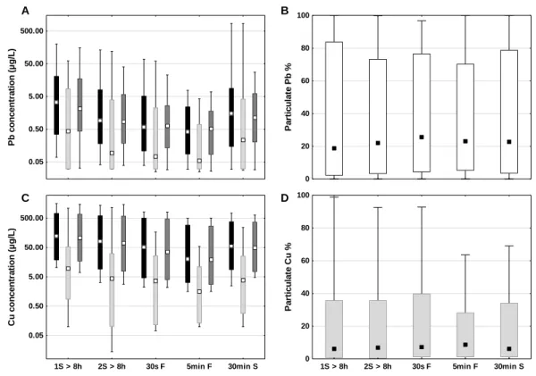
4.3.4 Particulate lead and copper ... 60
4.3.5 Particulate simulation sampling ... 62
4.3.6 Contributors to lead and copper concentrations ... 63
4.3.7 Blood lead levels modelling and copper intake ... 64
4.3.8 Possible remedial actions ... 66
4.3.9 Selecting a sampling protocol ... 68
4.4 Conclusions ... 70
CHAPTER 5 ARTICLE 2 – STUDY OF THE LONG-TERM IMPACTS OF TREATMENTS ON LEAD RELEASE FROM FULL AND PARTIALLY REPLACED HARVESTED LEAD SERVICE LINES ... 72
5.1 Introduction ... 73
5.2 Materials and methods ... 76
5.2.1 Pilot setup and operation ... 76
5.2.2 Sampling ... 78
5.2.3 Water quality monitoring ... 78
5.2.4 Statistical analysis ... 79
5.2.6 Field monitoring of LSL households ... 81
5.3 Results and discussion ... 81
5.3.1 Changes in total Pb concentrations over time ... 81
5.3.2 Impact of treatments on Pb concentrations after stagnation and under flow conditions 83 5.3.3 Impact of pipe configuration ... 87
5.3.4 Surface area-normalized mass release (SANMR) ... 87
5.3.5 Comparison of Pb release between pilot and field investigations ... 90
5.3.6 Managerial implication of partial LSL replacement ... 94
5.3.7 Options for utilities to decrease Pb concentrations ... 97
5.4 Conclusion ... 99
CHAPTER 6 ARTICLE 3 – LEAD AND COPPER RELEASE FROM FULL AND PARTIALLY REPLACED HARVESTED LEAD SERVICE LINES: IMPACT OF STAGNATION TIME PRIOR TO SAMPLING AND WATER QUALITY ... 101
6.1 Introduction ... 102
6.2 Materials and methods ... 105
6.2.1 Pilot setup ... 105
6.2.2 Sampling for lead and copper ... 105
6.2.3 Determination of lead and copper release rates ... 106
6.2.4 Scale analysis ... 107
6.2.5 Statistical analysis ... 107
6.3 Results and discussion ... 107
6.3.1 Copper concentrations after PLSLR simulation ... 107
6.3.2 Effect of stagnation time on copper concentrations ... 110
6.3.4 Impact of high velocity flushing ... 127
6.3.5 Implications for exposure to lead and copper ... 129
6.3.6 Implications for lead and copper sampling ... 129
6.3.7 Conclusion ... 133
CHAPTER 7 ONSET OF CHLORINATION, CHANGES IN ORTHOP DOSAGE IN FULL AND PARTIAL LEAD SERVICE LINES ... 134
7.1 Addition of chlorination ... 134
7.1.1 Lower CSMR and addition of chlorine ... 135
7.1.2 Increased pH and addition of chlorine ... 136
7.2 Changes in orthoP dosage ... 138
CHAPTER 8 CHANGES IN CORROSION SCALES IN FULL AND PARTIALLY REPLACED LEAD SERVICE LINES: IMPACT OF WATER QUALITY ... 141
8.1 General observations on scale formation ... 141
8.2 Do scales in 100%Pb pipes change with water quality? ... 143
8.2.1 Control condition and smaller diameter pipes ... 143
8.2.2 Sulfate addition with and without chlorine residual ... 145
8.2.3 Increase to pH 8.3 ... 147
8.2.4 orthoP ... 149
8.3 Are the scales present in the non-galvanic section of the Pb pipe affected by the presence of a downflow galvanic connection? ... 152
8.3.1 Control condition and smaller diameter pipes ... 152
8.3.2 Sulfate addition ... 155
8.3.3 Increase in pH ... 155
8.4 Which minerals are present in the galvanic zone of the partial LSL? How do copper
minerals differ between the galvanic and non-galvanic zones? ... 159
8.4.1 Control condition and smaller diameter pipes ... 159
8.4.2 Sulfate addition ... 161
8.4.3 Increase to pH 8.3 ... 162
8.4.4 orthoP ... 163
8.5 Can minerals confirm the presence of galvanic corrosion and indicate anodic/cathodic sites?.... ... 164
8.6 Concluding remarks ... 165
CHAPTER 9 GENERAL DISCUSSION ... 166
9.1 What are Pb and Cu sources in distribution systems? ... 169
9.1.1 Schools and large buildings ... 169
9.1.2 Lead service lines ... 171
9.2 What are the impacts of pH, chloride to sulfate mass ratio and orthophosphate on Pb and Cu?... ... 174
9.2.1 pH ... 174
9.2.2 Decrease of the CSMR ... 175
9.2.3 Addition of orthoP ... 175
9.3 Presence of particulate Pb ... 176
9.4 Is flushing an effective mitigation strategy to decrease Pb and Cu? ... 178
9.4.1 Schools and large buildings ... 178
9.4.2 Full and partial LSLs ... 179
9.5 What are the regulatory implications of the findings and how to sample for Pb and Cu?... ... 179
9.5.2 Lead service line ... 180
CHAPTER 10 CONCLUSION AND RECOMMENDATIONS ... 181
BIBLIOGRAPHY ... 185
LIST OF TABLES
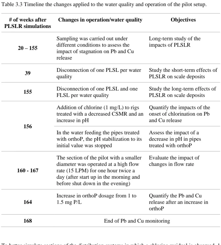
Table 3.1 Experimental approach to validate (or invalidate) the research hypothesis and corresponding chapters of the thesis. ... 27 Table 3.2 General water quality of the water entering the pilot setup, prior to addition of
treatments... ... 32 Table 3.3 Timeline the changes applied to the water quality and operation of the pilot setup. ... 35 Table 3.4 Description of pipes available for scale analysis. ... 38 Table 4.1 Information regarding buildings sampled, water quality and number of samples collected
per building. ... 47 Table 4.2 Percentage of samples with total Pb concentrations greater than 10 µg Pb/L and greater
than 5 µg Pb/L (in brackets), all types of samples considered at each type of tap and building…. ... 56 Table 4.3 Median, 90th percentile and maximum total Pb and Cu concentrations for a given type of
tap and group of building for all the samples, in µg/L. ... 59 Table 5.1 Corrosion control treatment, pipe configuration, and internal diameters tested in the pilot
setup as well as median and 90th percentile total Pb concentrations after 16HS and flowing condition. ... 77 Table 5.2 Apparent SANMR (total, dissolved and particulate Pb), expressed in µg/m2 under the
control condition for various experimental conditions tested compared to 6HS samples from the distribution system of the City of Montreal (Deshommes et al. 2016, 2017). ... 92 Table 5.3 Length of LSL (in m) at which total Pb mass from non-galvanic corrosion equals Pb
mass from galvanic corrosion. ... 97 Table 6.1 Total, dissolved, and particulate copper release rate (µg Cu/h) for the partial LSLs with
the Cu pipe upstream (Cu-Pb) and downstream (Pb-Cu) for the different treatments tested on the pilot setup. The release rate is presented for the first 16 hours of stagnation and from 24 to 336 hours (2 weeks) of stagnation. ... 115 Table 6.2 Total, dissolved, and particulate lead release rate (µg/h) for the full LSL (100%Pb) and
release rate is presented for the first 16 hours of stagnation, and from 24 to 336 hours (2 weeks) of stagnation. ... 122 Table 6.3 Median total Cu concentrations represented as X fold of the median concentration after
30 minute stagnation (30MS) and after 6 hour stagnation (6HS). ... 131 Table 6.4 Median total Pb concentrations represented as X fold of the median concentration after
30 minute stagnation (30MS) and after 6 hour stagnation (6HS). ... 132 Table 8.1 Lead corrosion solids identified in 100%Pb pipe for the control and smaller diameter
conditions, ++++ represents the major phases present in each sample, +++ moderate presence, ++ minor presence, + traces and D phases that were detected. ... 144 Table 8.2 Lead corrosion solids identified in 100%Pb pipe for the sulfate addition and the increase
in pH conditions, with and without chlorination, ++++ represents the major phases present in each sample, +++ moderate presence, ++ minor presence, + traces and D phases that were detected. ... 146 Table 8.3 Lead corrosion solids identified in 100%Pb pipe for addition o orthoP, before and after
the increase in dosage to 1.5 mg P/L, ++++ represents the major phases present in each sample, +++ moderate presence, ++ minor presence, + traces and D phases that were detected. .... 150 Table 8.4 Lead corrosion solids identified in Cu-Pb pipes for the control condition, ++++ represents
the major phases present in each sample, +++ moderate presence, ++ minor presence, + traces and D phases that were detected. ... 153 Table 8.5 Lead corrosion solids identified in Cu-Pb pipes for the smaller diameter pipes, ++++
represents the major phases present in each sample, +++ moderate presence, ++ minor presence, + traces and D phases that were detected. ... 154 Table 8.6 Lead corrosion solids identified in Cu-Pb pipes treated with sulfate addition, before and
after chlorination, ++++ represents the major phases present in each sample, +++ moderate presence, ++ minor presence, + traces and D phases that were detected. ... 156 Table 8.7 Lead corrosion solids identified in Cu-Pb pipes treated with an increase in pH to 8.3,
before and after addition of chlorination ++++ represents the major phases present in each sample, +++ moderate presence, ++ minor presence, + traces and D phases that were detected.
0-S indicates the pipe disconnected 30 weeks after PLSLR (short-term) and 0-L the pipe disconnected after 156 weeks, both treated with pH 8.3. ... 157 Table 8.8 Lead corrosion solids identified in Cu-Pb pipes treated with orthoP, before and after
increase in dosage, ++++ represents the major phases present in each sample, +++ moderate presence, ++ minor presence, + traces and D phases that were detected. 1-S indicates the pipe disconnected 30 weeks after PLSLR (short-term) and 1-L the pipe disconnected after 156 weeks, both treated with 1 mg P/L. ... 158 Table 8.9 Evidence of galvanic corrosion of the Pb pipe. ... 164 Table A.1 Overview of Canadian, American and European guidance and regulations on sampling lead and copper in schools are large buildings ... 200 Table A.2 Overview of studies on lead and copper in drinking water in large buildings, schools and
daycares ... 204 Table A.3 Percentage of the samples with a total Pb concentration greater than 1 µg Pb/L, all types
of samples considered at each types of tap and buildings. ... 214 Table A.4 Multivariate Adaptative Regression (MARSpline) results presenting significant
variables for total lead and copper concentrations. ... 215 Table A.5 Number of samples required to estimate the true geometric mean total Pb concentrations
LIST OF FIGURES
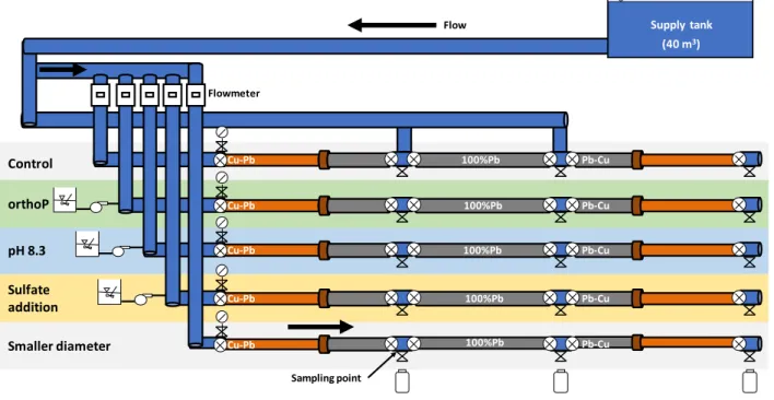
Figure 2.1 Schematic representation of reactions occurring in a galvanic couple comprised of lead and copper, adapted from Triantafyllidou and Edwards (2010). ... 11 Figure 3.1 Photograph of the pilot setup. ... 31 Figure 3.2 Schematic of the pilot setup installed in the CREDEAU Laboratory at Polytechnique
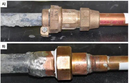
Montréal. ... 33 Figure 3.3 An example of a lead service line connected to a copper pipe using (A) a red brass
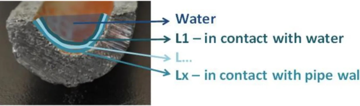
compression fitting and (B) a soldered fitting. ... 34 Figure 3.4 Example of a full LSL being prepared for scale analysis. ... 38 Figure 3.5 Cross-sectional representation of the different layers which can be present in the pipes. ... 39 Figure 3.6 Schematic representation of the corrosion zones present in a partial lead service line in
the presence of galvanic corrosion. ... 39 Figure 3.7 Samples mounted on a zero-background plate for XRD analysis: A) Sample placed in
the well of the plate, B) Sample mounted using amyl acetate. ... 40 Figure 4.1 Total, particulate and dissolved lead (A) and copper (C) concentrations (in black, light
grey and darker grey), and fraction of particulate Pb (B) and Cu (D), for 1st draw samples collected following overnight stagnation (1S>8h, 250 mL) and 2nd draw (2S>8h, 250 mL), 30 seconds (30sF, 250 mL) and 5 minutes (5minF, 250 mL) of flushing and 30 minutes of stagnation (30minS, 250 mL) (n=130).Whiskers represent min-max values, boxes 10th-90th percentiles, and the square represents median concentrations. ... 50 Figure 4.2 Total Pb and Cu concentrations (µg/L) for all taps sampled in schools without corrosion
control, low alkalinity (A for Pb and B for Cu), with corrosion control (C for Pb and D for Cu) and large buildings (E for Pb and F for Cu). Whiskers represent the min-max values and the line the median concentrations for the 5 samples collected at each tap, after stagnation (1S˃8h, 2S˃8h, 30minS) and flushing (30sF, 5minF). Vertical dotted lines separate the buildings sampled (B1 to B11). ... 52
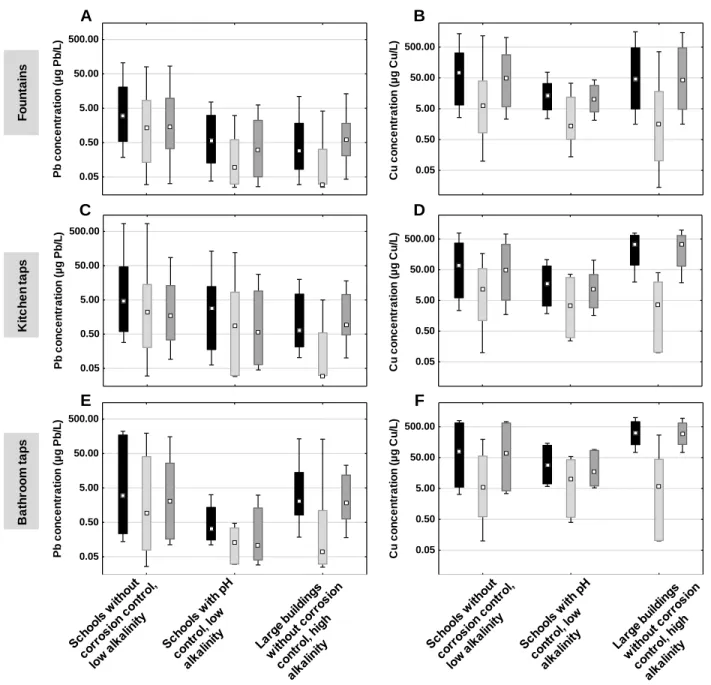
Figure 4.3 Total, particulate and dissolved lead and copper (in black, light grey and dark grey) for (A, B) fountains (n=385), (C, D) kitchen (n=140) and (E, F) bathroom (n=125) taps as a function of specific groups of buildings (all samples combined). ... 54 Figure 4.4 Particulate lead and copper concentration (A, C) and fraction (B, D) presented as
cumulative frequency for each type of building sampled. For A and C, the dark square represents the median, boxes represent the 10-90th percentiles, and whiskers the non-outlier range (n=130). ... 61 Figure 4.5 Mean total and particulate lead concentrations (in dark and light grey) for kitchen taps
sampled in elementary schools receiving low pH and low alkalinity water (N=7 taps in 5 schools). Black dots represent the mean Pb particulate fraction as a percentage. ... 63 Figure 4.6 Geometric mean BLL (grey boxes) for children of age 5-7 years for each group of
buildings, modeled using 90th percentiles total Pb concentrations observed in school tap water (black dots). ... 65 Figure 5.1 The apparent surface area-normalized mass release (SANMR), galvanic and non-galvanic zones present in lead (Pb) pipes connected to copper (Cu) pipes using a compression fitting (A). A partial lead service line (PLSL) from the pilot setup with a gap between the Cu and Pb pipe junction (B) and a PLSL where the Pb pipe is in direct contact with the Cu pipe (C). ... 80 Figure 5.2 Total lead (Pb) concentration after 16 hours of stagnation presented as a function of time
(in weeks) following partial lead service line replacement (PLSLR) simulation. Smaller diam.: smaller diameter pipe; orthoP: orthophosphate treatment. N=46 for Cu-Pb and Pb-Cu pipe configurations, N=60 for 100% Pb pipe configuration. ... 82 Figure 5.3 Total (A-B), dissolved (C-D) and particulate (E-F) lead (Pb) concentrations measured
after a 16 hour stagnation period (left) or under flowing conditions (right) under different corrosion control treatments. The 100% Pb pipe configuration is represented in grey, the Cu-Pb configuration in white and the Cu-Pb-Cu configuration with black dots. The line within each box represents the median concentration. The bottom and top of each box represents the 10th -90th percentiles, respectively. The whiskers represent the minimum and maximum values. 84
Figure 5.4 Example of a Pb-Cu pipe under the control condition showing external corrosion of the Pb and Cu pipes. ... 88 Figure 5.5 Apparent surface area-normalized masse release (SANMR) of total Pb for (A) 100% Pb
pipes, (B) Cu-Pb pipes and (C) Pb-Cu pipes is presented in dark grey. For PLSL (B and C), non-galvanic SANMR is presented in white and galvanic SANMR in light grey. The latter is calculated considering a 2 cm galvanic zone on the Pb and Cu pipes flanking the fitting, as well as the interior surface of the brass fitting. The galvanic SANMR was computed using median non-galvanic SANMR. ... 89 Figure 5.6 Mass of Pb released due to non-galvanic corrosion (grey), galvanic corrosion based on
median non-galvanic SANMR (orange and dotted) and the sum of both (black) in the Cu-Pb pipe configuration under the (A) control, (B) smaller diameter, (C) sulfate treatment, (D) orthoP treatment and (E) pH 8.3 conditions. ... 96 Figure 5.7 Framework for the management of full lead service Lines (FLSLs) and partial lead
service lines (PLSLs) in a distribution system. POU: point-of-use, SANMR: surface area-normalized mass release, PLSLRs: partial lead service line replacements, CCT: corrosion control treatment. ... 98 Figure 6.1 Total copper concentrations (µg Cu/L) after 16 hour stagnation inside the Cu pipe
section for partial LSLs with the Cu pipe: (A) upstream (Cu-Pb) and (B) downstream (Pb-Cu) of an aged Pb pipe as a function of the number of weeks after the simulation of a PLSLR. Median concentrations for different water qualities are presented: control condition (black square), sulfate addition (white triangle), orthoP dosing (star), and increase in pH to 8.3 (white diamond). The smaller diameter condition is represented by white squares. The whiskers represent the 10th and 90th percentile concentrations. ... 108 Figure 6.2 Copper concentrations (µg Cu/L) in the copper pipe section as a function of stagnation
time for partial LSLs in which the copper pipes are upstream of the Pb pipes (Cu-Pb). Median concentrations for different water qualities are presented: control condition (black square), sulfate addition (white triangle), orthoP dosing (star), and increase in pH to 8.3 (white diamond). The smaller diameter condition is represented by white squares. The whiskers represent 10th-90th percentile concentrations. ... 112
Figure 6.3 Copper concentrations (µg Cu/L) in the copper pipe as a function of stagnation time for partial LSLs in which the copper pipes are downstream of the Pb pipes (Pb-Cu). Median concentrations for different water qualities are presented: control condition (black square), sulfate addition (white triangle), orthoP dosing (star), and increase in pH to 8.3 (white diamond). The smaller diameter condition is represented by white squares. The whiskers represent 10th-90th percentile concentrations. ... 113 Figure 6.4 Lead concentrations (µg Pb/L) in the lead pipe section as a function of stagnation time
for full LSL (100%Pb). Median concentrations for different water qualities are presented: control condition (black square), sulfate addition (white triangle), orthoP dosing (star), and increase in pH to 8.3 (white diamond). The smaller diameter condition is represented by white squares. The whiskers represent 10th-90th percentile concentrations. ... 118 Figure 6.5 Particulate Pb fraction after different stagnation times for (A) 100%Pb, (B) Cu-Pb, and
(C) Pb-Cu. Median concentrations for different water qualities are presented: control condition (black square), sulfate addition (white triangle), orthoP dosing (star), and increase in pH to 8.3 (white diamond). The smaller diameter condition is represented by white squares. The whiskers represent 10th-90th percentile concentrations. ... 120 Figure 6.6 Lead concentrations (µg Pb/L) in the lead pipe section as a function of stagnation time
for partial LSLs in which the copper pipes are upstream of the Pb pipes (Cu-Pb). Median concentrations for different water qualities are presented: control condition (black square), sulfate addition (white triangle), orthoP dosing (star), and increase in pH to 8.3 (white diamond). The smaller diameter condition is represented by white squares. The whiskers represent 10th-90th percentile concentrations. ... 124 Figure 6.7 Lead concentrations (µg Pb/L) in the lead pipe section as a function of stagnation time
for partial LSLs in which the copper pipes are downstream of the Pb pipes (Pb-Cu). Median concentrations for different water qualities are presented: control condition (black square), sulfate addition (white triangle), orthoP dosing (star), and increase in pH to 8.3 (white diamond). The smaller diameter condition is represented by white squares. The whiskers represent 10th-90th percentile concentrations. ... 125 Figure 6.8 Total (grey) and particulate Pb (white) concentrations (µg Pb/L) for the smaller diameter
stagnation, (C) before increasing the flow rate, and (D) after increasing the flow rate (Q). Square: median concentrations, box: 10-90th percentiles, whiskers: min-maximum concentrations. ... 128 Figure 7.1 Total Pb concentrations as a function of the number of weeks following the simulation
of partial LSL replacements for the pipes treated with the addition of sulfate, before and after the onset of chlorination. Squares (Cu-Pb), triangle (100%Pb) and circles (Pb-Cu) represent median concentrations and whiskers represent minimum-maximum values. Pb pipes of full LSLs are 5 times longer than partial LSLs (3 and 0.6 m). N=46 and 11 for PLSL, N=60 and 22 for FLSL, before and after chlorination. ... 135 Figure 7.2 Dissolved Pb concentrations as a function of the number of weeks following the
simulation of partial LSL replacements for the pipes treated with the addition of sulfate, before and after the onset of chlorination. Squares (Cu-Pb), triangle (100%Pb) and circles (Pb-Cu) represent median concentrations and whiskers represent minimum-maximum values. Pb pipes of full LSLs are 5 times longer than partial LSLs (3 and 0.6 m). N=46 and 11 for PLSL, N=60 and 22 for FLSL, before and after chlorination. ... 136 Figure 7.3 Total Pb concentrations as a function of the number of weeks following the simulation
of partial LSL replacements for the pipes treated with the increase in pH to 8.3, before and after the onset of chlorination. Squares (Cu-Pb), triangle (100%Pb) and circles (Pb-Cu) represent median concentrations and whiskers represent minimum-maximum values. Pb pipes of full LSLs are 5 times longer than partial LSLs (3 and 0.6 m). N=46 and 11 for PLSL, N=60 and 22 for FLSL, before and after chlorination. ... 137 Figure 7.4 Dissolved Pb concentrations as a function of the number of weeks following the
simulation of partial LSL replacements for the pipes treated with the increase in pH to 8.3, before and after the onset of chlorination. Squares (Cu-Pb), triangle (100%Pb) and circles (Pb-Cu) represent median concentrations and whiskers represent minimum-maximum values. Pb pipes of full LSLs are 5 times longer than partial LSLs (3 and 0.6 m). N=46 and 11 for PLSL, N=60 and 22 for FLSL, before and after chlorination. ... 138 Figure 7.5 Total Pb concentrations as a function of the number of weeks following the simulation
of partial LSL replacements for the pipes treated with 1 mg P/L with pH adjustment, without pH adjustment and with an increase in orthoP dosage to 1.5 mg P/L. Squares (Cu-Pb), triangle
(100%Pb) and circles (Pb-Cu) represent median concentrations and whiskers represent minimum-maximum values. Pb pipes of full LSLs are 5 times longer than partial LSLs (3 and 0.6 m). N=46, 7 and 4 for PLSL, N=60, 12 and 8 for FLSL, before changes in treatment, after decrease in pH and after increase in orthoP. ... 139 Figure 7.6 Dissolved Pb concentrations as a function of the number of weeks following the
simulation of partial LSL replacements for the pipes treated with 1 mg P/L with pH adjustment, without pH adjustment and with an increase in orthoP dosage to 1.5 mg P/L. Squares (Cu-Pb), triangle (100%Pb) and circles (Pb-Cu) represent median concentrations and whiskers represent minimum-maximum values. Pb pipes of full LSLs are 5 times longer than partial LSLs (3 and 0.6 m). N=46, 7 and 4 for PLSL, N=60, 12 and 8 for FLSL, before changes in treatment, after decrease in pH and after increase in orthoP. ... 140 Figure 8.1 Example of surface layers with islands of red deposits (pipe treated with orthoP). ... 142 Figure 8.2 Photographs of the interior of a 100%Pb pipe from the control condition. ... 143 Figure 8.3 Interior deposits of a smaller diameter pipe. ... 143 Figure 8.4 Total, dissolved and particulate Pb concentrations after 16 hour stagnation in FLSL for
both pipes of the control condition. Line: mean concentration, boxes: mean ± SE, whiskers: minimum-maximum concentrations. N=31. ... 145 Figure 8.5 Full LSL treated with the addition of sulfate (A) and the combination of sulfate and
chlorine (B). ... 147 Figure 8.6 Full LSLs treated with an increase in pH (A and B) and an increase in pH combined
with chlorine (C and D). Picture on the right were taken with a stereomicroscope to enhance the details of the scale. ... 148 Figure 8.7 Total, dissolved and particulate Pb concentrations after 16 hour stagnation in FLSL for
both pipes of the increased pH condition with and without 1 mg Cl2/L. Line: mean concentration, boxes: mean ± SE, whiskers: minimum-maximum concentrations. ... 149 Figure 8.8 Full LSL fed with water dosed at 1 mg P/L (A and B) and 1.5 mg P/L (C and D). Pictures
Figure 8.9 Total, dissolved and particulate Pb concentrations after 16 hour stagnation in FLSL for pipes with the addition of orthoP before and after changes in dosage (1 vs 1.5 mg P/L). Line: mean concentration, boxes: mean ± SE, whiskers: minimum-maximum concentrations. ... 151 Figure 8.10 Partial LSL of the control condition (A) without visual changes in scale composition
at the galvanic zone and (B) with visual changes and for two duplicate pipes of the smaller diameter (C and D). ... 160 Figure 8.11 Interior of partial LSL treated with sulfate (A) and the combination of sulfate and
chlorine (B). ... 161 Figure 8.12 Partial LSL treated with an increased pH to 8.3 (A) and the combination of increased
pH and chlorine (B). ... 162 Figure 8.13 Interior of an orthoP treated partial LSL (A) shortly after PLSLR simulation, (B) before
changes in water quality and (C) after an increased in orthoP (1 vs 1.5 mg P/L). ... 163 Figure 9.1 Summary of the research conducted. ... 166 Figure 9.2 Factors influencing Pb release in a lead service line. ... 168 Figure A.1 Total lead concentration per type of tap and building sampled. Schools without corrosion control and with low alkalinity (A n=5, B n=20, C n=12), Schools with corrosion control and with low alkalinity (A n=3, B n=19, C n=7), Large buildings (A n=17, B n=38, C n=9). Whiskers represent minimum and maximum values, boxes the 10th and 90th percentile, white squares the median concentration. ... 212 Figure A.2 Total copper concentration per type of and building. Schools without corrosion control
and with low alkalinity (A n=5, B n=20, C n=12), Schools with corrosion control and with low alkalinity (A n=3, B n=19, C n=7), Large buildings (A n=17, B n=38, C n=9). Whiskers represent minimum and maximum values, boxes the 10th and 90th percentile, white squares the median concentration. ... 213 Figure B.1 Schematic of the pilot setup built using aged LSLs from the distribution system of
Montreal and new copper pipes connected to the Pb pipes using red brass compression fittings.. ... 219
Figure B.2 Total (A-B), dissolved (C-D) and particulate (E-F) lead (Pb) concentrations measured after a 16 hour stagnation period (left) or under flowing conditions (right) normalized for the length of the pipe for the control, smaller diameter, sulfate treatment, orthoP treatment, and pH 8.3 conditions. The 100% Pb pipe configuration is represented in grey, Cu-Pb configuration in white and Pb-Cu configuration with black dots. The line within each box represents the median concentration. The bottom and top of each box represents the 10th-90th percentiles, respectively. The whiskers represent the minimum and maximum values... 220 Figure C.1 Total (left) and dissolved (right) Cu concentration (µg/L) in the copper pipe depending
on stagnation time for the control condition (A and B) and the orthoP condition (C and D) in Cu-Pb pipe configurations (Cu pipes upstream of Pb pipes). Each colour/type of line represents consecutive sampling events. The full line (orange) is the 1st event, the long dashes (teal) the 2nd event and the short dashes (purple) the 3rd event. The triangles and the circles each represent one pipe. ... 223 Figure C.2 Total (left) and dissolved (right) Pb concentration (µg/L) in the lead pipe depending on
stagnation time for the control condition (A and B) and the orthoP condition (C and D), for the full LSLs (100%Pb). The squares, triangles, and circles each represent one pipe, as well as each colour/type of line. ... 224 Figure C.3 Total (left) and dissolved (right) Pb concentration (µg/L) in the lead pipe depending on
stagnation time for the control condition (A and B) and the pipes dosed with orthoP (C and D), for the partial LSLs in which the Cu pipe is upstream of the Pb pipe (Cu-Pb). The triangles and the circles each represent one pipe, as well as each colour. ... 225
LIST OF SYMBOLS AND ABBREVIATIONS
100%Pb Full lead service line16HS 16 hour of stagnation
1S>8h First draw sample after overnight stagnation 2S>8h Second draw sample after overnight stagnation
30minS 30 minute stagnation
30sF 30 second flush
3Ts Training, testing and telling
5minF 5 minute flush
6HS 6 hour of stagnation
A Alkalinity
AAP American Academy of Pediatrics
AI Aggressivity index
AL Action level
Al Aluminium
AMSARC Advanced Materials and Solids Analysis Research Core
ANOVA Analysis of variance
AO Aesthetic objective
AWWA American Water Works Association
BLL Blood lead level
°C Degree Celsius
CA California
Ca Calcium
CaCO3 Calcite
CC Corrosion control
CCT Corrosion control treatment
Cl2 Chlorine
cm Centimeter
CSMR Chloride to sulfate mass ratio
Cu Copper
Cu2Cl(OH)2 Clinoatacamite CuCO3Cu(OH)2 Malachite
Cu2O Cuprite
CuO Tenorite
Cu(OH,Cl)2 2H2O Calumetite CuOH2 Cupric hydroxide
Cu-Pb Partial lead service line with copper upstream of lead Cu4(SO4)(OH6)H2O Posnkjakite
CWN Canadian Water Network
Diss. Dissolved
DO Dissolved oxygen
EPA Environmental Protection Agency
EU European Union
Fe Iron
FLSL Full lead service line
GM Geometric mean
H Hardness
HC Health Canada
HCl Hydrochloric acid
HNO3 Nitric acid
ICP-MS Inductively coupled mass spectrometry
I.D. Internal diameter
IEUBK Integrated Exposure uptake biokinetic
L Liter
LCR Lead and copper rule
LPM Liters per minute
LSL Lead service line
m Meter
MAC Maximum acceptable concentration MARSpline Multivariate Adaptive Regression Splines
mL Milliliter
NA Not available
NOM Natural organic matter
NS Not specified
OH Ohio
OK Oklahoma
ON Ontario
ORP Oxidation reduction potential
orthoP orthophosphate
P Phosphate
PACl Polyaluminium chloride
Part. Particulate
Pb Lead
PbCO3 Cerussite
Pb3(CO3)2(OH)2 Hydrocerussite Pb10(CO3)6(OH)6O Plumbonacrite
Pb-Cu Partial lead serice line with lead upstream of copper
PbO Litharge
PbO2 Plattnerite
Pb3O4 Minium
Pb(OH)Cl Laurionite
Pb3(PO4)2 Tertiary lead phosphate Pb5(PO4)3(OH) Hydroxypyromorphite Pb5(PO4)3-Cl Chloropyromorphite
PbSO4 Anglesite
Pb4(SO4)(CO3)2(OH)2 Susannite / Leadhillite
PHG Public health goal
PLSL Partial lead service line
PLSLR Partial lead service line replacement PSS1 Particulate stimulation sampling, first liter PSS2 Particulate stimulation sampling, second liter PSS3 Particulate stimulation sampling, third liter PVDF Polyvinylidene Fluoride
PXRD Powder x-ray diffraction
QC Québec
RDT Random daytime
SI Supplementary Information
Sn Tin
SO4 Sulfate
TOC Total organic carbon
UK United-Kingdom
USA United States of America
USEPA United States Environmental Protection Agency USPSC United States Consumer Product Safety Commission
WHO World Health Organization
Zn Zinc
LIST OF APPENDICES
Appendix A Supplementary information, article 1: schools and large institutional buildings: Implications for regulation, exposure and management of lead and copper ... 199 Appendix B Supplementary information, article 2: Study of the long-term impacts of
treatments on lead release from full and partially replaced harvested lead service lines ... 218 Appendix C Supplementary information, article 3: Lead and copper release from full and
partially replaced harvested lead service lines: Impact of stagnation time prior to sampling and water quality ... 221
CHAPTER 1
INTRODUCTION – LEAD AND COPPER CORROSION
IN DRINKING WATER
1.1 Background
The presence of lead in drinking water has received unprecedented attention from the public since the scandal of Flint (Michigan, United States) was revealed in 2015 (Hanna-Attisha et al., 2016). Aside from being a probable carcinogen to humans (Health Canada, 2017; Silbergeld et al., 2000), lead is a neurotoxin linked to intellectual deficits in children (Jusko et al., 2008; Lanphear et al., 2005) and recently to cardiovascular disease mortality (Lanphear et al., 2018; Lustberg & Silbergeld, 2002; Schober et al., 2006). As environmental sources of lead have been reduced, drinking water has become one of the primary sources of exposure (Health Canada, 2017). Concerns associated with copper in drinking water are first aesthetic due to the blue water phenomenon (Edwards et al., 2000) as it can stain laundry and plumbing fixtures at concentrations below which there are health concerns (Health Canada, 2018). Despite being an essential element for humans, copper can also cause short and long-term health effects such as nausea, vomiting and diarrhea (WHO, 2004).
As water comes in contact with leaded plumbing components such as service lines, fixtures and solders, it becomes contaminated. Until 1975, lead service lines (LSL) were commonly installed in Canada and the use of solder containing lead was stopped in 1986 (Health Canada, 2017). At the time, “lead-free” was defined as containing less than 0.2% of Pb in solders and flux and 8% in pipes and pipe fittings. Since 2015 in the United States and 2014 in most Canadian provinces, no more than 0.25% of Pb must be found across the wetted surface of pipes, pipe fittings and fixtures (Health Canada, 2017; U. S. Government, 2011). Although these new standards will limit the use of leaded materials, utilities and building owners must manage a legacy of leaded materials. Recommended and regulated sampling protocols and action levels/maximum acceptable concentrations for lead and copper in drinking water in houses and in schools vary significantly in Canada, the United States and the European Union.
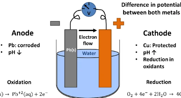
Amongst the different types of corrosion possible in plumbing components, uniform and galvanic corrosion are contributors to lead concentrations in tap water. Galvanic corrosion arises when two different metals of different nobility are in contact (Oldfield, 1988). As there is a difference in
potential between the two metals, a current flow is established, and each metal becomes either the anode or the cathode (Larson, 1975). The less noble metal, the anode, is oxidized and a decrease in pH can be observed compared to the conditions of the bulk water (Ma et al., 2017). The more noble metal, the cathode, becomes protected and oxidants are reduced at its surface and pH is increased (Larson, 1975; Oldfield, 1988). In presence of galvanic corrosion, the release of lead in water is increased (Dudi & Edwards, 2005; Edwards & Triantafyllidou, 2007; Schock & Lytle, 2011). Instances where the lead pipe was galvanically protected in a partial LSL have also been documented (Arnold & Edwards, 2012; DeSantis et al., 2018).
Alkalinity, pH, hardness, temperature, disinfectant residual, chloride to sulfate mass ratio (CSMR), dissolved oxygen and natural organic matter (NOM) are some of the factors affecting lead and copper solubility (Schock & Lytle, 2011). The presence of corrosion control treatments, such as orthophosphate or an increase in pH will also affect the extent of Pb and Cu leaching in water (Cardew, 2009; Cartier et al., 2013; Schock et al., 1995). Empirical galvanic series define that copper is more noble than brass and that lead is the less noble of the 3 metals (Matsukawa et al., 2010). When galvanic couples are formed between lead, brass and/or copper, lead is preferentially corroded and a drop in pH can be observed at its surface. Changes in local water quality are reflected in modifications in the scale composition (DeSantis et al., 2018).
Recent studies highlighted the impact of drinking water at schools on the blood lead levels (BLL) of children (Deshommes et al., 2016a; Sathyanarayana et al., 2006; Triantafyllidou et al., 2014). Multiple North American studies have demonstrated high and varying lead concentrations in tap water in large buildings and some also reported elevated copper levels. In a meta-analysis of Canadian schools and large buildings, Deshommes et al. (2016a) demonstrated that Pb levels vary depending on the sampling protocol, with highest concentrations measured in the first draw after extended stagnation and reaching a maximum concentration of 13,200 µg Pb/L in one specific case. Lower concentrations were measured after 30 minutes of stagnation, as it was the case in a school investigated in New Jersey when concentrations were measured after 10 minutes of flushing followed by a random stagnation time (Murphy, 1993). Studies also report that flushing the tap prior to drinking water reduced the Pb and Cu concentrations (Barn et al., 2014; Boyd et al., 2008b; Triantafyllidou et al., 2014). However, there is no published study on the impact of water quality, type of taps where samples are collected and sampling protocol on Pb and Cu concentrations in schools and large buildings.
The number of LSLs in the United States is estimated to range between 5.5 and 7.1 million, providing water to 15 to 22 million Americans (Cornwell et al., 2016). In Canadian and American cities with population ranging between 24,000 and 3,000,000 inhabitants, up to 69,000 LSLS are still present (Deshommes et al., 2018a). According to the same study, utilities stopped installing LSLs between 1930 and 1975. In most instances, due to share ownership of the service line between the utility and the homeowner, only the public section of the LSL can be removed when municipalities are conducting replacement. It results in partial LSL replacements (PLSLR) in which the private section of the LSL remains as is. Regulatory agencies are also making full LSL replacement mandatory. As an example, the Michigan Department of Environmental Quality requires full LSL replacement, at the expense of the utilities, within the next 20 years (Department of Environmental Quality of State of Michigan, 2018). Field studies conducted in North American cities using different water qualities, report that Pb concentrations increase shortly after PLSLR and then decrease to levels comparable to before the replacement or to lower levels (Deshommes et al., 2016a; Deshommes et al., 2017; Muylwyk et al., 2011; Swertfeger et al., 2006). Short and long-term pilot studies have shown the importance of corrosion inhibitors, flow rate, type of couplings, stagnation time prior to sampling and water quality on the release of particulate Pb in partial LSLs (Cartier et al., 2012a; Cartier et al., 2013; Kogo et al., 2017; St. Clair et al., 2016; Triantafyllidou & Edwards, 2011; Wang et al., 2012; Wang et al., 2013; Zhou et al., 2015).
1.2 Structure of the dissertation
This thesis is divided in 10 chapters. A review of the state of the literature on the presence of lead and copper in drinking water distribution system is presented in Chapter 2. It is followed (Chapter 3) by the presentation of the research objectives as well as a short overview of the methodology used. Chapter 4 through Chapter 6 present research results in the form of 3 submitted or published scientific publications. The first article (Chapter 4, published in Water Research) investigates the sources of lead and copper in schools and large institutional buildings as well as the impact of water quality, type of taps and sampling protocols on concentrations measured. The focus of the dissertation then moves on to the presence of lead and copper in service lines, at pilot scale. The second article (Chapter 5, submitted to Water Research) reports the long-term trends in lead release following simulation of partial LSL replacements and proposes a framework for the management of full and partial LSL. The third article (Chapter 6 , submitted to Water Research), presents the
trend in copper concentrations following partial LSL replacements and investigates the use of different stagnation times prior to sampling for lead and copper. The changes in lead leaching associated with changing flow velocity are also investigated. Chapter 7 presents the impact of the onset of chlorination on lead release in full and partial LSLs, as well as the increase in orthophosphate dosage. The next chapter (Chapter 8) reports the changes in scale composition and relative abundance between full and partial LSLs, under different water qualities. Chapter 7 and Chapter 8 will be submitted for publication at a later date. Finally, a general discussion on galvanic corrosion and the release of lead and copper is presented in Chapter 9 and is followed by conclusions and recommendations (Chapter 10).
CHAPTER 2
LITERATURE REVIEW
2.1 Health impacts of lead and copper
2.1.1 Lead
Changes in water quality in Flint (Michigan, United States) and Washington, D.C. (United States) resulted in increases in blood lead levels (BLL) of children as water lead levels rose (Brown et al., 2011; Hanna-Attisha et al., 2016). Triantafyllidou and Edwards (2012) listed 14 studies, published between 1977 and 2009, clearly linking drinking water to increased BLLs. With decreasing environmental exposure to lead, drinking water is now a major source of exposure (Health Canada, 2017). Elevated BLLs are of concerns as there are no levels of exposure that are considered to be safe (Bellinger et al., 1992; Needleman, 2004; WHO, 2011) and exposure to low levels of Pb in water result in a significant increase in BLLs (Ngueta et al., 2016). Indeed, intellectual deficits arise at low levels of exposure to lead (Bellinger, 2008; Canfield et al., 2003; Health Canada, 2013; Lanphear et al., 2005) and children have a higher uptake of lead than adults, 40-50% vs 3-10% respectively (Manton et al., 2000; Mushak, 1998; Ziegler et al., 1978). Exposure to lead has also been linked to cardiovascular disease mortality in the United States (Lanphear et al., 2018; Lustberg & Silbergeld, 2002; Schober et al., 2006).
2.1.2 Copper
Despite being an essential element for humans, ingesting concentrations of copper greater than 3,000 µg Cu/L was shown to cause nausea, abdominal pain or vomiting in healthy adults (Pizarro et al., 1999; WHO, 2004). Infants (<1 year old) are the most at risk of copper toxicity as their body has not yet developed homeostatic mechanisms required to clear copper and prevent its intestinal entry (Georgopoulos 2001; Müller-Höcker et al., 1988). However, health impacts arise at concentrations greater than those at which there are aesthetic impacts, which include staining the laundry and plumbing fixtures (Edwards et al., 2000). Interestingly, Swedish researchers showed that daily copper requirements could be met only from drinking tap water (Pettersson & Rasmussen, 1999). Overall, health issues that are associated with exposure to copper appear to be of less concern than those associated with lead exposure.
2.2 Recommendations/Regulations on lead and copper in drinking
water
Sampling protocols for lead and copper, as wells as maximum acceptable concentrations (MAC) and action levels (AL) are different in Canada, the United States and the European Union. Also, the Canadian government can only provide recommendations for sampling and acceptable concentrations, as drinking water standards are regulated by provinces and territories. Also, some regulatory agencies provide specific requirements for lead and copper sampling in schools and daycares, while others only provide protocols for general sampling in the distribution system. The same sampling protocol is applied for lead and copper in many jurisdictions, raising concerns about the effectiveness of such an approach as dissolution dynamics as well as effects of temperature are different for both metals (Lytle & Schock, 2000; Masters et al., 2016). The appropriate estimation of particulate Pb is also a concern associated with lead sampling and the handling of samples (Deshommes et al., 2016a; Triantafyllidou et al., 2014; Triantafyllidou et al., 2007).
2.2.1 Canada
In 2017, Health Canada issued new proposed recommendations concerning lead sampling in houses, suggesting sampling after 30 minutes of stagnation or random day time (RDT) rather than after at least 6 hours of stagnation as in the previous recommendations. Also, the proposed MAC is decreased from 10 µg Pb/L to 5 µg Pb/L (Health Canada, 2009, 2014, 2017). Maximum copper concentration allowed in drinking water are based on aesthetic objectives as it can stain the laundry and plumbing fixtures. As such, aesthetic objectives (AO) are recommended for copper as well as MAC based on health effects. Health Canada recommends an AO of 1,000 µg Cu/L as well as a newly proposed MAC of 2,000 µg Cu/L (Health Canada, 2018).
Multiple Canadian provinces, such as Alberta, Québec and Manitoba require that samples for lead, in houses and in schools, be collected after flushing the taps and their MAC are in line with current adopted Canadian Guidelines (Table A.1). Whereas Ontario requires sampling targeted to schools and daycares which includes collecting samples after at least 6 hour stagnation, as well as after 30 minutes of stagnation at every outlet used by children (Government of Ontario, 2017, 2018).