HAL Id: hal-01183951
https://hal.archives-ouvertes.fr/hal-01183951
Submitted on 12 Aug 2015
HAL is a multi-disciplinary open access
archive for the deposit and dissemination of
sci-entific research documents, whether they are
pub-lished or not. The documents may come from
teaching and research institutions in France or
abroad, or from public or private research centers.
L’archive ouverte pluridisciplinaire HAL, est
destinée au dépôt et à la diffusion de documents
scientifiques de niveau recherche, publiés ou non,
émanant des établissements d’enseignement et de
recherche français ou étrangers, des laboratoires
publics ou privés.
Robust k-coverage algorithms for sensor networks
Gyula Simon, Miklos Molnar, László Gönczy, Bernard Cousin
To cite this version:
Gyula Simon, Miklos Molnar, László Gönczy, Bernard Cousin. Robust k-coverage algorithms for
sensor networks. IEEE Transactions on Instrumentation and Measurement, Institute of Electrical and
Electronics Engineers, 2008, 57 (8), pp.1741-1748. �10.1109/TIM.2008.922072�. �hal-01183951�
Robust k-coverage algorithms for sensor networks
Gyula Simon1, Miklós Molnár2, László Gönczy3, Bernard Cousin2 1 Department of Computer Science, University of Pannonia,
H-8200, Veszprém, Egyetem u. 10, Hungary
2 IRISA, Campus de Beaulieu, 35 042 Rennes Cedex, France
3 Dept. of Measurement and Information Systems, Budapest University of Technology and Economics
H-1117 Budapest, XI. Magyar tudósok krt. 2., Hungary
Email: [email protected], {molnar, bcousin}@irisa.fr, [email protected]
Abstract – Robustness, fault tolerance, and long lifetime are key requirements of sensor networks used in real-world
applications. Dense sensor networks with high sensor redundancy offer the possibility of redundant sensing and low duty-cycle operation at the same time, thus the required robust sensing services can be provided along with elongated lifetime. In this paper the Controlled Greedy Sleep Algorithm is analyzed. With low local communication overhead the proposed algorithm is able to solve the k-coverage sensing problem while it effectively preserves energy in the network. In addition, it can adapt to dynamic changes in the network such as node failures. The quality of service (network-wide k-coverage) is guaranteed independently of communication errors in the network (as long as it is physically possible); message losses affect only the network lifetime. Node failures may cause temporary decrease in the coverage service. The robustness of the algorithm is proven and its behavior is illustrated by simulation examples.
Keywords – sensor network, k-coverage, dependable, sleep-scheduling. I. INTRODUCTION
Wireless sensor networks are constructed from small, autonomous sensors and are utilized for various measurement purposes. The individual power capacity of the sensors is very limited (using batteries they may last only some days) but the expected useful lifetime of the network is required to be in the range of weeks or months, depending on the application. To achieve network longevity low duty cycle operation is utilized. In continuously operating sensor networks redundant sensors are deployed from which only a little subset is active at a time; the major part of sensors is turned off and thus energy is preserved. In redundant dense sensor networks various scheduling algorithms are used to control energy conservation.
In sensor networks used to austerely monitor an area in space it may also be a requirement that multiple sensors be able to provide measurements from each point in space. This property may either be necessary because of the applied measurement technology, safety or performance reasons or to satisfy accuracy requirements with relatively low-quality sensors. High redundancy present in the network is necessary to achieve this goal. In general this class of problems can be treated as the k-coverage problem, where k-coverage means the ability of a sensor to perform measurements over a certain area. While in a dense sensor network there may be several good solutions to the general k-coverage problem, the energy conservation criterion narrows the range of the acceptable solutions.
In many applications coverage is satisfactory as soon as the required level of coverage is reached, so higher coverage does not provide better performance or better application service. Thus finding an ‘economical’ solution to the k-coverage problem with small number of participating nodes results in energy conservation and longer network lifetime as well. Effective scheduling algorithm is required to organize the alternation of active (awake) and sleeping sensor sets to provide continuous service of the network.
In this paper the recently proposed Controlled Greedy Sleep Algorithm, which is capable of providing dependable k-coverage and prolonged network lifetime at the same time [#1] is reviewed and its robustness properties are analyzed and formally proven. In Section II the main related previous results are summarized. Section III reviews the Controlled Greedy Sleep Algorithm. In Section IV the fault tolerance properties of the algorithm are analyzed and the robustness of the algorithm is proven.
II. PREVIOUS RESULTS
Because of their fragility and power deprivation the dependability of sensor networks is an important and hot research topic. There are several propositions to ensure fault tolerance at different levels [#2]. Since the sensors are performing both sensing
and communication tasks the main problems of sensor networks are associated to these two activities [#3]. The sensor network should be capable of taking measurement in the observed area and transmitting the measured values to sink nodes. The k-coverage problem is associated with measurement functionality [#4]: every point of the target area must be covered by at least
k sensors (k is determined by the application). It also has several implications to connectivity issues [#5]. In real cases one can
suppose that the communication radius of the sensors is at least twice of the sensing radius. So, if the observed area is fully covered by active sensors, then the same sensors guarantee a connected network to data transmission as well.
The life-time of the network is generally prolonged by scheduling sleep intervals for some sensors, meanwhile the continuous service is provided by the active sensors (see examples in [#6], [#7], [#8]). The lifetime longevity and the network operability require efficient trade-offs, realized by different scheduling algorithms, which can mainly be divided into two main groups: random and coordinated scheduling algorithms [#9]. A distributed, random sleeping algorithm was proposed in [#10] where nodes make local decisions on whether to sleep or to join a forwarding backbone, to ensure communications. Each node’s decision is based on an estimate of how many of its neighbours will benefit from its being awake and the amount of energy available to it.
In [#11] the authors propose a randomized, simple scheduling for dense and mostly sleeping sensor networks. They suppose that there are many redundant sensors in the target area and one can compute the required (identical) duty cycle for individual sensors. In the proposed Randomized Independent Sleeping algorithm, time is divided into periods. At the beginning of each period, each sensor decides whether to go to sleep (with probability p computed from the duty cycle) or not, thus the lifetime of the network is increased by a factor close to 1/p. This solution is very simple and does not require communication between sensors. The drawback of the proposition is that there is no guarantee for coverage nor for network connectivity. Furthermore, since the sleeping factor is the same for all sensors, this solution cannot adapt to inhomogeneous or mobile sensor setups.
To handle the basic coverage problem the authors in [#9] propose a Role-Alternating, Coverage-preserving, Coordinated Sleep Algorithm (RACP). Each sensor sends a message periodically to its neighbourhood containing its location, residual energy and other control information. An explicit acknowledgment-based election algorithm permits to decide the sleep/awake status. The coordinated sleep is more robust and reduces the duty cycle of sensors compared to the random sleep algorithm. It guarantees 1-coverage in the network when it is physically possible. In this solution the topology can affect the behaviour; thus the sensors can adapt their sleeping to the needs. The price of the performance is the significant communication overhead increasing power consumption.
In [#12] the asymptotic behavior of coverage in large-scale sensor networks is studied. For the k-coverage problem, formulated as a decision problem, polynomial-time algorithms (in terms of the number of sensors) are presented in [#4]. A comprehensive study on both coverage and connectivity issues can be found in [#13].
In [#1] new coordinated algorithms were proposed to guarantee k-coverage in the network where it is physically possible and at the same time provide prolonged network lifetime. The proposed algorithms take into account both the power status and the placement (sensing assignment) of the sensors by periodically computing a “drowsiness factor” for each sensor. The drowsiness factor is used to schedule the sleeping or awake status of the sensors. The centralized version of the algorithm requires network-wide communication and thus it is expensive in large networks. A distributed approximation was also proposed that uses only locally available information. The Controlled Greedy Sleep Algorithm requires only a few messages to be broadcasted locally from every node to the direct neighbors in each period. Thus the energy wasted on the communication overhead is small, compared to the gain in the total energy saving in the network, supposing the period of the scheduling is sufficiently large. In the next section the Controlled Greedy Sleep Algorithm will be reviewed and then its robustness will be analyzed. Major novel contribution of this paper is this robustness analysis and proofs of correct behavior even in the presence of faults.
III. CONTROLLED GREEDY SLEEP (CGS) ALGORITHM
A. Background
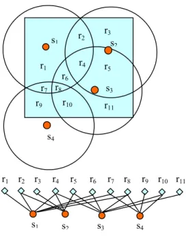
The sensing assignment in a sensor network can be represented by a bipartite graph G
(
RUS,E)
, where the two disjoints sets of vertices represent the nodes S and geographical regions R (see Fig. 1). The regions are defined by the subset of sensors that can monitor them. Generally, the regions cover the whole measured area and are disjoint. In G there is an edge e between region r∈ and sensor R s∈ if and only if s (completely) covers region r. SThe simple k-coverage problem is to find a sub-graph G′
(
RUS′,E′)
where S′⊆S so that for all vertices R in G′ thedegree is at least k.
The minimal k-coverage problem is to find a non-redundant sub-graph G′ that solves the k-coverage problem with minimal number |S’| of sensors. A graph G′ is non-redundant if there exists no G′′
(
RUS′′,E′′)
and S′′⊂S′ that solves the simplesets. Similarly to the Minimal Cover Vertex Set problem [#14], finding the minimal set of sensors k-covering all regions is an NP-complete optimization problem.
The goal of the sensor network k-coverage scheduling algorithms is even more complex than the computation of static minimal k-covering sets: these algorithms aim to prolong the lifetime of the sensor network with the help of the alternation of appropriate k-covering sets minimizing the power consumption and thus maximizing network lifetime.
A new, empirical factor based scheduling algorithm has been proposed recently in [#1]. In the centralized solution of the proposition, G may be known and used by the coordinator node, but in a distributed solution nodes have local information on their neighborhood only. Thus instead of G each sensor node q will use a locally known sub-graph Gq
(
RqUSq,Eq)
. This sub-graph contains geographical regions R covered by q , the set of sensors q S including node q and those of its neighbors qthat cover at least one region of R , and edges q E with an edge e between region q r∈Rq and sensor s∈Sq if and only if s
covers region r.
B. Assumptions
Assumption 1. The communication radius of the sensors is at least twice of the sensing radius. In most practical cases it’s a
sensible assumption and it automatically provides network-wide communication if 1-coverage in sensing is provided [#8]. Generally, from the assumption it also follows that network connectivity is higher than k when sensing k-coverage is provided [#5]. From this assumption it trivially follows that sensors covering at least one region of R are inside the communication q
radius of q.
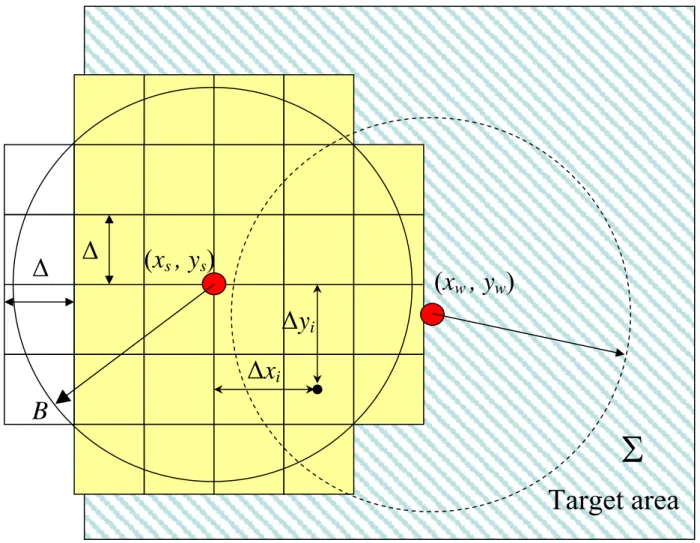
Assumption 2. For the sake of simplicity we assume that the coverage of each sensor can be modeled by a sensing disk and a
corresponding sensing radius B (we use a constant sensing radius but this has no essential effect on the algorithm). Within its sensing radius a sensor is able to perform measurements, while outside the sensing circle the sensing performance may degrade (but not necessarily).
An easily computable approximation of the sensing disk by a set of squares is illustrated in Fig. 2, where 32 square regions are used. We denote by
Δ
the side length of the square region. Let’s denote the location of node s by (xs, ys), and the center ofregion i by
(
Δ ,xi Δyi)
in the node’s local coordinate system. The graph G will contain regions s R shown in Fig. 2 (note that sthe regions only partially covered are also included here); S includes node s s and the neighbors of s ; E includes edges s
between s and all regions in R , and an edge between region s i∈Rs and a neighbor node w∈Ss placed at location (xw, yw) if
node w fully covers region i . A possible simplification can be the following: there is an edge between node w and region i if
(
) (
2)
2 2 2 w i s w i s x x y y y x B− Δ> +Δ − + +Δ − . (1)The square model may seem a rude approximation of the sensing disk, but since the sensing disk model is inherently a rather imperfect estimation of the real sensing area of a sensor, there is no point to put great effort to accurately approximate it. Note that a node always tries to provide coverage for all the regions it partially covers, but assumes that another node covers a region only if fully covers it. This solution is pessimistic, i.e. certain areas may be unnecessarily over-covered.
Assumption 3. The sensors know their own coordinates and the observed area Σ . Thus the sensors handle only regions that
are (at least partly) inside of Σ , as shown in Fig. 2.
Note that the algorithm can handle localization errors, provided the location uncertainties are small versus the sensing radius. If the maximum location error is lΔ , then (1) has to be modified to assure the correct behavior of the algorithm as follows:
(
) (
2)
2 2 2 2 l xs xi xw ys yi yw B− Δ − Δ> +Δ − + +Δ − . (2)The modification reflects the worst case when the distance error between sensors s and w is the maximal value 2Δl. C. Quality of Service Metrics
The first (functional) requirement the algorithm must provide is coverage: the network must maintain k-coverage of the largest possible part of the area. The second (non-functional) requirement is long network lifetime. The performance of the
network can be characterized with the size of the fully covered regions. A possible metric Θ can be the k-coverage-ratio k defined as A Ak k = Θ , (3)
where A is the area of the k-covered regions and A is the total area of the target space Σ . If the regions have approximately k
the same size then another similar metric Θ′ can be defined to approximate k Θ : k
N Nk k =
Θ′ , (4)
where Nk is the number of the k-covered regions while N is the total number of regions in the target space.
In a critical application the k-coverage must be maintained as long as possible and with Θ as high as possible. If in a k degrading network Θ is not satisfactory any more it may still be important to maintain a high value for k Θk−1, Θk−2, etc, e.g. in order to provide full connectivity in the remaining network.
The k-lifetime Lk(λ) of a network can be defined as the maximum operational time of the network with Θk >λ, where 1
0<λ≤ (close to 1 in practice).
D. Controlled Greedy Sleep (CGS) Algorithm
The following robust, fault tolerant, distributed algorithm solves the k-coverage problem using locally available information only and thus its communication overhead is low, as opposed to the centralized solution presented in [#1]. The basic idea is similar to that of the centralized solution: The network operates in periods; the awake/sleeping nodes are elected at the beginning of each period. A drowsiness factor is used to represent both the sensor’s energy status and its “importance” in the network. While in the centralized solution a central coordinator node controlled the election process based upon the drowsiness of all nodes in the network, in the distributed solution each node decides on its own status based on its own and its neighbors’ drowsiness. The drowsiness factor of node s with remaining energy E is defined as follows: s
⎪ ⎩ ⎪ ⎨ ⎧ − ∀ > Φ Φ = ∀
∑
∈ otherwise 1 0, if 1 r E Ds s r R r r s α , (5)and α is a positive constant (e.g. α=2), and Φ is the coverage ratio of region r defined as follows: r ⎪⎩ ⎪ ⎨ ⎧ − > − = Φ otherwise 1 if 1 K c K cr r r (6)
where cr is the degree of region r in G . The coverage ratio s Φ is positive if the region is over-covered, i.e. more than k r
sensors could cover region r. Φ is negative if region r is not over-covered: in this case the operation of all sensors possibly r
covering r is essential.
The drowsiness factor Ds takes into account the energy of sensor s: the smaller the energy of a sensor the larger its
drowsiness. A sensor participating in many regions that have low over-coverage is likely to participate in more possible solutions than sensors covering regions also covered by many other sensors. Thus a heuristic criticality property is included in
Ds to increase the lifetime of the network: sensors participating in regions only slightly over-covered have larger drowsiness.
The drowsiness factor for each sensor includes the sum of the coverage ratios of the regions the sensor is able to observe. This property enforces the sensors in critical positions to go to sleep whenever it is possible, to conserve their energy for times when their participation will become inevitable. With the design parameter α the balance between the energy and criticality can be adjusted; we used α=2in all the simulations. Note that negative drowsiness indicates that the sensor is not allowed to sleep.
The core of the operation can be summarized as follows: when a node decides on its status it will greedily opt for sleeping if the k-coverage problem can be solved by other nodes that either have been elected to stay awake or have lower drowsiness. The order of decision is based on the drowsiness factor, which serves as a priority metric.
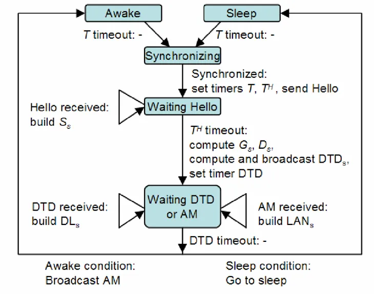
1. Run the network for a period of T, the coverage is provided by the awake sensors. 2. All sensors in the network wake up at the end of each period and synchronize.
3. Nodes with remaining energy level high enough for at least one more period of operation broadcast local Hello messages containing their node locations. Based on received Hello messages each node s builds up its local set of alive neighbor
4. After time TH, based on the received Hello messages each node s generates the local bi-partite graph
(
)
s s s s R S E G U , using Assumption 2, and then it calculates its drowsiness factor Ds.5. Based on Ds each node s selects a Decision Time Delay (DTDs). Small drowsiness means large DTD, large drowsiness
means small DTD. These delays provide priorities when nodes announce their Awake Messages.
6. Each node s broadcasts its DTDs and starts collecting other nodes’ DTD and Awake Messages (AMs). From the received
DTD messages each node s builds a Delay List (DLs), and from the received AMs it builds a List of Awake Neighbors
(LANs).
7. After DTDs time elapsed each node s makes a decision based upon LANs and DLs:
− if all regions in R can be k-covered using only nodes present in LANs s and/or nodes q present in DLs for which DTDq
> DTDs then s goes to sleep
− otherwise stay awake and broadcast an AM to inform other nodes that node s will stay awake.
In step 7 nodes go to sleep in a greedy manner: if the coverage problem can be solved with the already known awake neighbors in the LAN (due to their higher drowsiness factor these nodes have decided earlier on their awake status) and some of the neighbors with lower drowsiness factor (these nodes will decide their sleep/awake status later) then the node greedily elects to sleep and leaves the problem to those already being awake and those who haven’t decided their status yet. The operation of the algorithm is illustrated by a state machine in Fig. 3.
The communication overhead of the algorithm is low. In each cycle every node broadcasts only at most three messages (two if the node will go to sleep, three otherwise) in addition to the synchronization messages in step 2 (if needed). The nodes must stay awake in order to complete the election process, and during this extra Te time nodes consume energy. The communication
and awake-time overhead can be neglected if T is significantly longer than Te, which is true in most practical cases. Further
decrease of the communication overhead is possible by choosing T as long as possible. The length of T is limited by the need of the alternation of the k-covering sensor sets and/or the dynamics of the network (the scheduling should respond to the dynamic changes). This latter optimization problem on the length of T is out of the scope of this paper.
The nodes must be synchronized to provide optimal performance, but as will be discussed in Section 4.C, the algorithm is very robust against synchronization errors. For time synchronization purposes any of the solutions available in the literature, can be used, e.g. Flooding Time Synchronization Protocol, which provided less than 5 sμ average synchronization error per hop in challenging real multi-hop setups [#15].
IV. FAULT TOLERANCE OF THE CGS ALGORITHM
In this section, first we prove that our algorithm can provide k-coverage, and then we analyze the behavior of the algorithm facing message loss, sensor failures and synchronization errors.
A. Fault model
Nodes make their decision based upon received Hello, DTD, and Awake messages. In real circumstances messages can be lost due to various reasons: collision, fading, external disturbances, etc. In this study we assume that any of the above messages can be lost (in worst case all of the messages in the network may be lost). We also assume that received messages are correct (it can easily be ensured using error detecting coding in the messages) and no Byzantine error sources are present (this can be ensured by secure channels) [#16]. Also, the effect of synchronization errors will be discussed.
B. Guaranteed coverage
In this section the fault tolerant properties of the CGS algorithm will be proven. In the proof two lemmas will be utilized: Lemma 1 states that if there is a feasible solution to k-cover the whole sensing area then a solution can be found in a distributed way as well. Lemma 2 presents an important property of the algorithm: if k-coverage is feasible for all of the regions R s
supervised by a sensor s, then the k-coverage in this area is still possible after s makes a decision (sleep or stay awake) according to CGS. Using these results Theorem 1 proves that assuming fault free sensors, the CSG algorithm finds a feasible solution to k-cover the observed area if a solution exists at all.
Definitions: The k-coverage problem is solvable if the network-wide k-coverage (Θk =1) can be provided with the
available sensors. The sensor is available if it is alive (has enough energy) and is not sleeping. We assume that the problem is solvable at the time of network startup. Recall that S is the set of neighbors of sensor s participating in the sensing activity s
of regions in which s can make measurements. The solvability problem can be decided in a distributed fashion in the following way.
Lemma 1. If and only if it is true for all s that each region in R corresponding to s s can be k-covered using the available
sensors in S then the k-coverage problem can be solved with the available sensors. s Proof of the Lemma 1.
On one hand, if the k-coverage problem is solvable in all of the regions in R for all s s , then the k-coverage of the whole
area Σ is solvable. Let i
S be the set of available sensors to k-cover the region ri∈Σ. Trivially, the area s s i i R r U U = = Σ .
The union of the sets i i
S
S*=U thus k-covers Σ . On the other hand, if a region r in the seti R cannot be sufficiently covered s
by the available sensors in S then there are no other available sensors in the network to help, since according to Assumption s
1 a sensor must be the neighbor of s to be able to cover any region inR . ■ s
Lemma 2. If the k-coverage problem is solvable using the available sensors before Step 7 of the algorithm, then after Step 7
the problem remains solvable.
Proof of Lemma 2. If sensor s decides to stay awake in Step 7 then the sleeping status of the network is unchanged, thus in
this case the problem trivially remains solvable after Step 7.
If sensor s opts for sleeping then according to Step 7, sensors in LANs and sensors q in DLs with DTDq > DTDs could
cover all regions in R . It’s easy to show that these sensors are truly awake when s makes its decision: According to the fault s
model the information stored in LANs and DLs is correct (but not necessary complete). Thus the sensors in LANs are surely
awake since they are the sensors that have already decided to stay awake (but not necessarily all awake neighbors are in LANs
due to lost messages). Likewise, at the moment s executes Step 7 every sensor q in DLs with DTDq > DTDs is still awake
since it will decide on its sleeping status after time DTDq - DTDs (but again not necessarily all DTD messages are received and
this list may be incomplete). Thus the set of sensors s relies on is a subset of truly available sensors, so after Step 7 R really s
can be k-covered by them. Note that in our fault model the available sensor set is supposed to be failure free during the election process. Following from Lemma 1 if the k-coverage problem was solvable before Step 7 then each region in R can be k-p
covered using the available sensors in S , for all sensors p . Since the sleeping status of p s affects only regions in R (which s
also remained k-covered) then applying Lemma 1 again in the reverse direction it follows that the k-coverage problem is still solvable for the whole network. Thus independently of the decision of sensor s the problem is still solvable after Step 7. ■
Theorem. If physically possible (i.e. the coverage problem can be solved with the available sensors) the algorithm will
provide Θk =1.
Proof of Theorem. We assume that the k-coverage problem can be solved with the set of all available sensors in the network
at the beginning of the election process. Nodes in the CGS algorithm can go to sleep only in Step 7, thus the other steps do not affect the solvability of the k-coverage problem. There are a finite number of nodes in the network, so after s
s DTD
max time all nodes eventually execute Step 7 and decide whether to sleep or stay awake. According to Lemma 2, after the final decision the problem is still solvable, meaning that the k-coverage problem can be solved with the available (still awake) sensors. Since the set of available sensors will not change until the next period, the coverage is provided. ■
C. Effect of lost messages
Although the coverage is provided by CGS regardless of the message loss in the network while it is possible, lost messages naturally have negative effect on the performance. The CGS algorithm uses three types of messages, we evaluate successively the effects caused by the loss of each of them.
Lost Hello messages prevent the inclusion of neighbors in the alive neighbor set S , thus the drowsiness factor will be s
unnecessarily high and potential covering sensors are not considered when the local k-coverage is computed. When a node receives a DTD message from a neighbor without having previously received the associated but lost Hello message, the election process will take into account the unexpected DTD message. Lost DTD messages are harmful when the lost DTD is higher than that of the would-be recipient’s; in this case the sender is not considered as potential participant in the coverage, handicapping nodes with higher drowsiness. When a node receives an AM message from a neighbor without having previously received the associated but lost DTD message, the election process will take into account the unexpected AM message. Lost AMs result in potential over-coverage because nodes making decisions cannot rely on the presence the senders of these messages.
Lost messages cause over-coverage with unnecessarily high number of sensors staying awake and thus communication failures result in the shortening of network lifetime. The effect will be illustrated in Section V.
D. Effect of node failures
A node failure may happen in any of the four main states of our CGS algorithm: during an awake period, during a sleep period, during the Hello phase of the election process, and during the DTD phase of the election process. If a node fails during its awake period and it was covering a not over-covered region then naturally that region will remain under-covered until the end of the period. If physically possible, the next election will provide sufficient coverage again. If a node fails during its sleep period, it was not covering any region thus obviously the coverage is unchanged. If a node fails during its Hello phase, then the CGS behavior is equivalent to the loss of Hello messages (which has been evaluated above). The only situation a failing node can cause problem during the election process is when the node dies right after having transmitted its DTD message. In this case nodes with higher drowsiness factor may incorrectly rely on the presence of the failed node. Naturally, node failures generally cause the shortening of the lifetime of the network, since both the possible coverage in certain regions and the total amount of energy in the network decreases.
E. Effect of time synchronization errors
In this section the effect of the synchronization errors will be discussed.
If a node is out of synchronization but wakes up while the synchronization phase is running then it can synchronize again and continue its operation. If the node cannot synchronize it will stay awake till the next synchronization period, thus providing extra coverage in its neighborhood.
To ensure the proper operation of the CGS algorithm the participating nodes must be loosely synchronized, but there are no strict requirements. The synchronization period must be long enough to enable all nodes wake up and join the synchronization. Small timing errors have no effect on the Hello and DTD messages. The only part of the algorithm where timing is critical is the Decision Time Delay and the broadcast of AM. Timing errors may cause AM messages to be sent later or earlier than other nodes expect them. On algorithmic level this may cause change of priority for some nodes, but it has no effect on the provided k-coverage (but naturally may effect network lifetime).
In general, large timing errors may cause large message delays and ultimately message losses, but the algorithm is very tolerant in this respect, as was shown in Section IV.C.
Although time synchronization errors do not affect the provided k-coverage, they still can shorten the network lifetime and thus for optimal performance a synchronization service must be use. In a typical application, where T is in the range of several minutes or even hours, a few seconds of waiting for the network wakeup is acceptable. FTSP [#15], for example, is able to provide accuracy in the range of milliseconds even in very large networks, which is several orders of magnitude better than required.
V. RESULTS
The proposed CGS algorithm and the random k-coverage algorithm [#11] were simulated in Prowler, a probabilistic sensor network simulator [#17]. The simulator parameters were set to model the Berkeley MICA motes’ MAC layer [#18]. The radio propagation model includes realistic effects, e.g. fading, collisions and lost messages.
The tests were performed with a well controlled setup containing 100 nodes placed uniformly on a 10x10 grid, plus 2 extra nodes in each corner (total 108 nodes). The distance of adjacent nodes on the grid was 10 m, the sensing radius was 15 m, and the communication radius was approximately 40 m. In the simulation the initial energy of all sensors was set to 20 units and in each period awake sensors consumed 1 unit of energy. The period T was set to 1 hour and the required coverage was k=3.
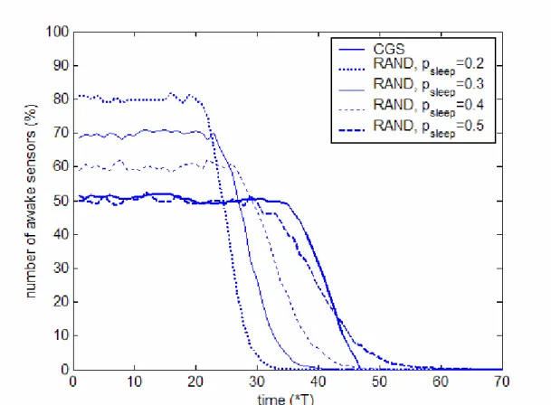
If all the nodes were awake in the network the network would operate for exactly 20 periods. In Fig. 4 the performance of the random k-coverage and the CGS algorithms can be compared. The plots show k-coverage ratios Θ for k = 3, as a function k of time. The difference is clearly visible: the CGS algorithm provided much better quality of service (Θ3 =1 while if was possible) and a much longer network lifetime: 3-koverage was provided for 36 periods in the experiment. For small sleep probabilities the random algorithm provided 3-coverage for almost 100% of the observed area but the network lifetime was only slightly higher than 20 periods. For higher sleep probabilities (psleep =0.5) the lifetime of the network is comparable to that of the CGS but with much lower coverage ratio (around 85%).
The number of awake sensors is shown, as a function of time, in Fig. 5. As it is expected, for the random algorithm the ratio of the awake sensors is 1−psleep, before the nodes start to die. In the experiment for the CGS algorithm this ratio is
approximately 50% (this is the reason why the random algorithm with psleep =0.5 has similar lifetime). Obviously, the CGS algorithm provides guaranteed high quality service and long network lifetime at the same time.
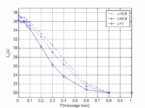
Fig. 6 shows the L3
( )
λ network 3-lifetime for different λ values as a function of message loss, for the experimental setup. The plots show the averaged result of 100 experiments. With large message loss probability all of the sensors stay awake all the time thus the network lifetime is reduced to 20 periods. With zero message loss the network lifetime is increased by approx. 85% (with respect to 20 periods) in the example. As the message loss rate increases the k-lifetime decreases almost linearly. Above 50% of message loss rate the performance of the algorithm is severely degraded. With the practically important message loss rates (up to 10%) the algorithm improves the network k-lifetime with 70% (>34 periods vs. 20 period), even for1 =
λ , i.e. for 100% required coverage ratio, when compared to the random solution. VI. SUMMARY
A distributed algorithm was proposed to solve the k-coverage problem and to provide prolonged network lifetime. The proposed periodic scheduling of sleeping and awake nodes saves energy in the network and extends overall network lifetime. The Controlled Greedy Sleep Algorithm guarantees k-coverage in the whole network whenever the topology of the network permits it. The algorithm requires only a few messages to be broadcasted from every node in each period, thus the energy wasted on the communication overhead is small, compared to the gain in the total energy saving in the network, supposing the period of the scheduling is sufficiently large
The CGS algorithm is robust and fault tolerant: the algorithm provides the required coverage network-wide (when possible) independently of node failures or even high amount of lost messages. With the help of the alternation of active sensor sets, the scheduling can adapt to dynamic changes in sensor conditions. The algorithm was compared to the random k-coverage algorithm and was proved to be superior in two senses: while it is possible, the CGS algorithm guarantees the required coverage all over the network. Also, the degradation curve is much gentler, thus the network service is provided for a longer time.
The fault tolerant behavior of the algorithm was proven and was illustrated by simulation examples: independently of the amount of message loss in the network the algorithm always provides the required coverage. The network lifetime degrades proportionally with the message loss rate, according to simulation results.
ACKNOWLEDGMENT
This research was partially supported by “Dependable, intelligent networks” (F-30/05) project of the Hungarian-French Intergovernmental S&T Cooperation Program and by the Hungarian Government under contract NKFP2-00018/2005.
REFERENCES
[#1] G. Simon, M. Molnár, L. Gönczy, and B. Cousin, “Dependable k-coverage algorithms for sensor networks, ” in Proc.
IMTC 2007, 2007.
[#2] F. Koushanfar, M. Potkonjak and A. Sangiovanni-Vincentelli, “Fault Tolerance in Wireless Ad Hoc Sensor Networks,” IEEE Sensors, Vol 2, pp. 1491-1496, 2002.
[#3] N. Ahmed, S.S. Kanhere and S. Jha, “The holes problem in wireless sensor networks: a survey,” SIGMOBILE Mob. Computer Communication Revue, Vol. 9, No. 2, pp. 4-18, 2005.
[#4] C.-F. Huang, and Y.-C. Tseng, “The coverage problem in a wireless sensor network,” in Proc. WSNA’03, 2003. [#5] H. M. Ammari and S. K. Das, “Coverage, connectivity, and fault tolerance measures of wireless sensor networks,” in
Proc. 8th Int. Symp. on Stabilization, Safety, and Security of Distributed Systems (SSS), LNCS 4280, pp. 35-49, 2006.
[#6] R. Krashinsky and H. Balakrishnan, “Minimizing energy for wireless web access with bounded slowdown,” in Proc.
MobiCom '02, 2002, pp. 119-130.
[#7] L.S. Brakmo, D.A. Wallach and M.A. Viredaz, “Sleep: a technique for reducing energy consumption in handheld devices,” in Proc. MobiSys '04, 2004, pp. 12-22.
[#8] G. Xing, X. Wang, Y. Zhang, C. Lu, R. Pless and C. Gill, “Integrated coverage and connectivity configuration for energy conservation in sensor networks,” ACM Transactions on Sensor Networks, vol. 1, No 1, pp. 36-72, 2005.
[#9] C. Hsin and M. Liu, “Network coverage using low duty-cycled sensors: random & coordinated sleep algorithms,” in Proc.
of the Third International Symposium on Information Processing in Sensor Networks, 2004, pp. 433-442.
[#10] B. Chen, K. Jamieson, H. Balakrishnan and R. Morris, “Span: An Energy-Efficient Coordination Algorithm for Topology Maintenance in Ad Hoc Wireless Networks,” Wireless Networks, Vol 8. No 5, pp. 481-494, 2002.
[#11] S. Kumar, T. H. Lai and J. Balogh, “On k-coverage in a mostly sleeping sensor network,” in Proc. MobiCom '04, 2004, pp. 144-158.
[#12] B. Liu and D. Towsley, “A study of the coverage of large-scale sensor networks,” in Proc. 1st IEEE Int. Conf. on
Mobile Ad-hoc and Sensor Systems (MASS), 2004.
[#13] A. Ghosh and S. K. Das, “Coverage and connectivity issues in wireless sensor networks,” Mobile, Wireless and Sensor Networks: Technology, Applications and Future Directions, (Eds. R. Shorey, et al.), Wiley-IEEE Press, Mar. 2006. [#14] M. R. Garey and D. S. Johnson. “Computers and Intractability; A Guide to the Theory of NP-Completeness,” W. H.
Freeman & Co., New York, NY, USA, 1990.
[#15] M. Maróti, B. Kusy, G. Simon, and A. Lédeczi, “The flooding time synchronization protocol,” in Proc. SenSys '04, 2004, pp. 39-49.
[#16] C. Karlof, N. Sastry and D. Wagner, “TinySec: A Link Layer Security Architecture for Wireless Sensor Networks,” in
Proc. SenSys '04, 2004, pp. 162–175.
[#17] G. Simon, P. Völgyesi, M. Maróti and A. Lédeczi, “Simulation-based optimization of communication protocols for large-scale wireless sensor networks,” in Proc. 2003 IEEE Aerospace Conference, 2003. Simulator can be downloaded from http://www.isis.vanderbilt.edu/Projects/nest/prowler/
[#18] J. Hill and D. Culler, “Mica: A Wireless Platform for Deeply Embedded Networks,” IEEE Micro, Vol. 22, No. 6, pp. 12–24, 2002.
Fig. 1. An example of the target area covered by four sensors (s1, …, s4).
The sensing disks and the sensing regions (r1, …, r11) are also shown, along with the corresponding bipartite graph.
s2 s3 s4 r1 r2 r3 r4 r 5 r6 r7 r8 r9 r10 r11 s2 s1 s1 s3 r1 r2 r3 r4 r5 r6 r7 r8 r9 r10 r11 s4
Fig. 2. Possible approximation of the sensing disk of sensor s by a set of rectangular regions in Rs (lightly shaded); regions
outside the target area (striped) are not handled. In E there is an edge between region s i∈Rs and neighbor node w∈Sssince
region i is fully covered by node w .
Δx
i
(x
s
, y
s
)
Δ
Δy
i
Δ
Target area
Σ
B
(x
w
, y
w
)
Fig. 4. Degradation of QoS characteristics of the CGS and the random algorithms with different psleep values. The required coverage was k=3.