HAL Id: tel-01157144
https://tel.archives-ouvertes.fr/tel-01157144
Submitted on 27 May 2015HAL is a multi-disciplinary open access
archive for the deposit and dissemination of sci-entific research documents, whether they are pub-lished or not. The documents may come from teaching and research institutions in France or abroad, or from public or private research centers.
L’archive ouverte pluridisciplinaire HAL, est destinée au dépôt et à la diffusion de documents scientifiques de niveau recherche, publiés ou non, émanant des établissements d’enseignement et de recherche français ou étrangers, des laboratoires publics ou privés.
Copyright
search for geo-neutrinos: studying electron antineutrinos
with Double Chooz and Borexino
R. Roncin
To cite this version:
R. Roncin. From the measurement of the θ13 mixing angle to the search for geo-neutrinos: studying electron antineutrinos with Double Chooz and Borexino. High Energy Physics - Experiment [hep-ex]. Université Paris Diderot (Paris 7) Sorbonne Paris Cité; Università degli Studi dell’Aquila, 2014. English. �NNT : 2014PA077141�. �tel-01157144�
ED 560 - STEP’UP - “Sciences de la Terre de l’Environnement et Physique de l’Univers de Paris”
Università degli Studi dell’Aquila
Thèse de Doctorat / Tesi di Dottorato
Physique des Particules / Fisica delle Particelle
From the measurement of the ✓
13
mixing
angle to the search for geo-neutrinos:
studying ¯⌫
e
with Double Chooz and Borexino
présentée par
Romain Roncin
pour l’obtention des titres de
Docteur de l’Université Paris Diderot (Paris 7) Sorbonne Paris Cité Dottore dell’Università degli Studi dell’Aquila
Thèse dirigée par Pr Alessandra Tonazzo / Dr Francesco Villante Laboratoire AstroParticule et Cosmologie / Laboratori Nazionali del Gran Sasso
soutenue publiquement le 29 septembre 2014 devant le jury composé de :
Dr Jacques Dumarchez Président du jury Pr Alessandra Tonazzo Directrice de thèse Dr Francesco Villante Directeur de thèse
Pr Masaki Ishitsuka Rapporteur
Dr Gioacchino Ranucci Rapporteur
Dr Anatael Cabrera Co-encadrant de thèse
à mon frère, à ma soeur, à Globule et à toi, Margaux
Acknowledgments
J’ai bien conscience que les quelques pages qui vont suivre seront certainement les plus lues, au moins pour les non-anglophones, aussi je vais tenter de m’appliquer. J’ai toujours pensé qu’écrire ces pages coulerait de source. Il n’en est rien. Trouver pour chacun d’entre vous les mots justes n’est pas chose aisée. Je vais ici abandonner l’anglais pour retrouver ma bien-aimée langue maternelle. Il y a beaucoup de personnes que je voudrais remercier, je vais certainement en oublier et j’en suis par avance désolé.
Je ne suis pas certain de l’ordre protocolaire qu’il me faut respecter mais je voudrais commencer par remercier les directeurs des laboratoires dans lesquels j’ai pu étudier dans des conditions, il faut le reconnaître, optimales. Je remercie Pierre Binétruy et Stavros Kat-sanevas du laboratoire AstroParticule et Cosmologie (APC) ainsi que Stefano Ragazzi du Laboratori Nazionali del Gran Sasso (LNGS).
Je remercie les membres du jury d’avoir accepté d’en faire partie. Merci à Masaki Ishit-suka et Gioacchino Ranucci d’avoir accepté d’être les rapporteurs de cette thèse et à Jacques Dumarchez d’avoir présidé ce jury. Certains pourraient vous dire que je n’ai pas la mémoire des évènements mais croyez bien que le 29 septembre 2014 restera à jamais gravé dans ma mémoire.
Je voudrais continuer en remerciant mes directeurs de thèse, et ils sont nombreux ! Je re-mercie Aldo Ianni et Francesco Villante de m’avoir si bien accueilli et encadré au Gran Sasso. Cette expérience a été inoubliable. Je remercie ensuite Anatael Cabrera sans qui la partie light noise de cette thèse n’aurait jamais pu aboutir. Je me souviens du soulagement que j’ai éprouvé après ton coup de téléphone m’annonçant que les coupures light noise avaient été approuvées par la collaboration. Je tiens enfin à exprimer toute ma gratitude à ma directrice de thèse, Alessandra Tonazzo, qui m’a tellement apporté que j’ai bien conscience que les mots employés ici ne sont pas assez forts pour exprimer combien je te suis reconnaissant. Tu as été la directrice de thèse idéale. Depuis mon stage de L3 jusqu’à cette thèse en passant par les summer student programmes du DESY et du CERN, c’est toi qui m’a guidé au fil de toutes ces années et je t’en remercie !
Cela me permet d’enchaîner en remerciant Thomas Patzak, sans qui je n’aurais pas connu Alessandra. A l’époque de la L3, je cherchais un stage et c’est toi qui m’a orienté vers Alessan-dra... et Michel Cribier ! Merci Michel, merci d’être toi ! J’ai appris énormément à tes côtés
dire, en écrivant ces lignes, j’ai déjà hâte que tu passes pour parler de tout et de rien. Merci Michel, merci.
Je remercie l’ensemble du groupe neutrinos de l’APC. Merci à Antoine Kouchner, Jaime Dawson, Didier Kryn, Hervé de Kerret, Michel Obolensky, Alberto Remoto et Kazuhiro Terao. Un merci particulier à Daniel Vignaud qui m’a suivi tout au long de ces trois années. Je remercie les équipes du CEA avec qui j’ai pu échanger. Merci à David Lhuillier et Thierry Lasserre qui m’ont fait grandir. J’ai appris beaucoup à vos côtés. J’en profite égale-ment pour remercier Matthieu Vivier, Vincent Fischer et Valérian Sybille. Tu m’as beaucoup fait rire durant cette dernière année de thèse ! C’est vraiment dommage que tu ne sois pas arrivé plus tôt !
Ce qu’il y a de bien dans les collaborations comme celle de Double Chooz, c’est qu’au-delà d’être collègues, on forge des amitiés. Merci Antoine Collin ! Les meetings de collaboration vont me manquer, c’est certain ! Les shifts peut-être un peu moins, quoique, c’était quand même bien sympa, j’en garde en tout cas de bons souvenirs. Merci Guillaume Pronost ! Tu m’as vraiment beaucoup aidé avec ce boulot prenant qu’est DataMigro, surtout sur la fin ! On en aura passé des heures sur Skype, au téléphone, à Chooz et même jusqu’à Montréal à réparer, réparer et encore et toujours réparer DataMigro. Merci d’avoir été là Guillaume, j’ai toujours pu compter sur toi. Tu m’as vraiment été d’une aide précieuse.
En parlant d’aide précieuse, je remercie Pau Novella avec qui je troquais du français con-tre de la physique. Merci d’avoir pris le temps de relire des parties de ce manuscrit, tu m’as beaucoup appris et je t’en suis très reconnaissant. Merci à Paolo Agnes et Adrien Hourlier d’avoir réussi à me supporter dans ce bureau, surtout sur la fin. Merci à Simona Soldi avec qui je partageais toujours le premier “bonjour” en arrivant à l’APC et qui m’a aidé à affronter certains déboires liés à l’administration italienne.
A propos d’administration, je remercie Martine Laird-Bardissa, Martine Piochaud, Lu-dovic Davila, Marie Verleure et Sabine Tesson qui m’ont toujours apporté leur aide quand j’en avais besoin. Merci à vous tous. J’en profite également pour remercier Annette sans qui les shifts et les meetings de collaboration n’auraient pas eu la même saveur.
Je tiens maintenant à remercier Luca Agostino, Stefano Perasso et Davide Franco. Merci de m’avoir accompagné pendant ces trois années. Je me souviens Davide me remontant le moral après la publication des premiers résultats de Daya Bay, je me rappelle Stefano prenant du temps pour discuter de tout et de rien et je me rappelle Luca étant présent au quotidien, jour après jour, à partager les joies et les moments un peu plus difficiles de la thèse. Merci à tous les trois, si je garde d’aussi bons souvenirs de ces trois années, c’est sans aucun doute que vous y êtes pour quelque chose.
Merci à mes partenaires de UT, de QPUC et de tennis du mardi matin 8h. Je remercie les “vieux” thésards Loïc, Alexandre et Marie-Anne. Je tiens également à remercier mes amis Julian, Matthieu, Benjamin, Maïca et Alexis d’avoir réussi à me supporter tout au long de ces trois années. Je remercie mes amis du NPAC avec qui c’est toujours un plaisir d’aller boire un verre. Un grand merci à Pierre, Guillaume, Aurélien, Patrick, Flavien, Alice et Asénath. J’en profite également pour remercier Isabelle et Assina, merci d’être venues à ma soutenance. Je tiens maintenant à remercier mes collègues du LNGS. Merci à Francesco Lombardi et Marcin Misiaszek d’avoir été là pour moi dès le premier jour. Ces quelques mois passés en Italie ont été formidables et c’est en grande partie grâce à vous et à la bonne ambiance qui régnait dans ce bureau. Je tiens également à remercier Chiara Ghiano, Yura Suvorov, Nicola Rossi et George Korga.
Ces trois années de thèse n’auraient pas eu la même saveur sans le monitorat que j’ai effectué au sein du Palais de la Découverte. Merci à Kamil Fadel et Hassan Khlifi de m’avoir accueilli et de m’avoir fait confiance. Je remercie Sigfrido Zayas et Alain de Botton d’avoir toujours su donner un éclat particulier à ces journées passées là-bas. J’adresse enfin un grand merci à Alice (encore) pour avoir été ma binôme pendant ces trois années, cette expérience au Palais de la Découverte n’aurait pas été la même sans toi.
Je remercie du fond du cœur mes amis angevins qui m’ont apporté un soutien réconfortant quand j’en avais le plus besoin et qui m’ont eux aussi beaucoup fait rire (c’est quoi theta treize ?) mais aussi réfléchir, en particulier Emilie et Meihdi. Merci à Ano, Clairette, Steph, Guil-laume, Nicolas, Eléonore, Hermine, Wilfried et Maryline. Merci à Sylvain et Carole d’avoir toujours été présents et à Fanny d’être toujours à mon écoute depuis toutes ces années.
Je remercie Jean-Pierre, Françoise et Louise, ainsi que Françoise et Juliette, de s’être in-téressés à mon travail et de m’avoir offert ces moments de repos à Lugon-et-l’Ile-du-Carnay, Bordeaux ou encore Lacanau. Je remercie également les grand-mères de Margaux, Suzanne et Kelly, d’avoir toujours pris de mes nouvelles.
Je remercie mon papa et ma maman qui m’ont toujours apporté leur soutien même s’ils ne devaient pas toujours comprendre ce que je faisais ! Merci du fond du cœur d’être de si bons parents ! Je remercie mon frère et ma sœur, ce manuscrit vous est en partie dédié. J’en profite également pour remercier Christelle.
En vrac, je voudrais aussi remercier Kavinsky, Daft Punk (j’en ai écrit du code sur vos chansons), Arto Paasilinna, Donald Westlake (rien de mieux que de vous lire pour se vider la tête), la dame à la gare de Tokyo qui m’a gentiment orienté dans ce labyrinthe, les dames d’easyJet qui ne m’ont jamais fait payé mes surplus de valises, les gardes italiens du Gran Sasso qui savent tellement bien prononcer mon nom de famille (Ronccchhhine). Je remercie ma Peugeot 205, Titine pour les intimes, de ne pas nous avoir fait faux-bond lors de notre
Je voudrais maintenant remercier un être cher qui nous a malheureusement quitté il y a peu, notre chat, Globule. Merci d’avoir été si tendre dans les moments difficiles de la thèse.
Je souhaiterais clore ces quelques pages en remerciant celle qui est à mes côtés depuis toutes ces années, Margaux. Merci de m’avoir supporté, de m’avoir encouragé, de m’avoir permis de me dépasser. Jour après jour tu as su croire en moi et pour tout cela je te remercie infiniment.
Contents
Introduction 1
1 Neutrinos: History and Physics 3
1.1 Birth certificate . . . 3
1.2 Chasing the different neutrino species . . . 5
1.2.1 ¯⌫e, a two steps discovery . . . 5
1.2.2 ⌫µ discovery . . . 7
1.2.3 ⌫⌧, looking for the “kink” . . . 8
1.2.4 How many neutrino families? . . . 9
1.3 Solar neutrino anomaly . . . 9
1.3.1 The Sun, a neutrino factory . . . 10
1.3.2 Chasing solar neutrinos . . . 12
1.3.3 Solving the anomaly . . . 14
1.4 Atmospheric neutrino anomaly . . . 15
1.5 Unsolved anomalies . . . 18
1.5.1 Reactor antineutrino anomaly . . . 18
1.5.2 GALLEX and SAGE, the gallium anomaly . . . 19
1.5.3 LSND and MiniBooNE anomalies . . . 20
2 Deepening the neutrino knowledge 23 2.1 Neutrinos within the Standard Model . . . 24
2.1.1 Masses in the Standard Model: the Higgs mechanism . . . 25
2.2 Neutrino masses . . . 26
2.2.1 Dirac mass term . . . 26
2.2.2 Majorana mass term . . . 27
2.2.3 See-saw mechanism . . . 28
2.2.4 Neutrino masses from experiments . . . 29
2.3 Neutrino mixing and oscillation . . . 31
2.3.1 Neutrino mixing . . . 32 2.3.2 Neutrino oscillation . . . 32 2.3.3 Solar sector, m2 21and ✓12 . . . 37 2.3.4 Atmospheric sector, m2 32 and ✓23 . . . 39 2.3.5 ✓13 sector . . . 39 2.4 Cosmological informations . . . 46
2.5 Sterile neutrinos? . . . 46
3 The Double Chooz experiment 49 3.1 Principle . . . 50
3.1.1 From the ¯⌫e emission... . . 50
3.1.2 ... to their detection . . . 52
3.1.3 Oscillation measurement concept . . . 54
3.2 Experiment design . . . 55
3.2.1 Detector design . . . 56
3.2.2 Data acquisition system . . . 61
3.2.3 Calibration system . . . 63
3.3 Event reconstruction . . . 64
3.3.1 Energy reconstruction . . . 64
3.3.2 Vertex position reconstruction . . . 66
3.4 Backgrounds studies . . . 67
3.4.1 Correlated background . . . 67
3.4.2 Uncorrelated background . . . 68
4 Dealing with an unexpected background 71 4.1 Motivations . . . 71
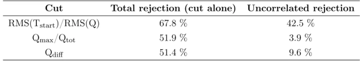
4.2 Discriminating variables . . . 72
4.2.1 PMT Time RMS variable . . . 72
4.2.2 PMT Charge RMS variable . . . 73
4.2.3 Maximum PMT Charge over Total Charge variable . . . 73
4.2.4 Q variable . . . 74
4.3 Strategy . . . 74
4.4 Validation of the strategy . . . 82
4.4.1 Cross-check with calibration source . . . 82
4.4.2 Cross-check with MC . . . 84
4.4.3 Cross-check with special runs . . . 84
5 Measuring ✓13 with Double Chooz 87 5.1 Neutrino selection . . . 88
5.1.1 Gd-capture sample selection . . . 88
5.1.2 H-capture sample selection . . . 94
5.2 Systematic uncertainties . . . 96
5.2.1 Gd-capture systematics . . . 96
5.2.2 H-capture systematics . . . 100
5.3 Reactor-off data analysis . . . 101
5.3.1 Signal prediction . . . 102
5.3.2 Reactor-off measurement . . . 102
5.4 ✓13 measurements . . . 103
5.4.1 Rate and spectral shape analysis . . . 103
6 Looking for geo-neutrinos with Borexino 115
6.1 Borexino: from the Sun to the Earth . . . 116
6.1.1 Experimental site and detector design . . . 116
6.1.2 Solar neutrinos in sight . . . 117
6.2 A unique opportunity to study geo-neutrinos . . . 119
6.2.1 A look at the Earth . . . 119
6.2.2 Geo-neutrinos production . . . 121
6.2.3 Geo-neutrino signal prediction . . . 125
6.3 Chasing the geo-neutrinos . . . 127
6.3.1 Detection . . . 127 6.3.2 Selection . . . 128 6.4 Background studies . . . 131 6.4.1 Reactor background . . . 131 6.4.2 Accidental background . . . 131 6.4.3 Cosmogenic background . . . 132
6.5 Maximum likelihood analysis . . . 133
7 Neutrino directionality studies 139 7.1 Neutrino directionality motivations . . . 139
7.2 Neutrino directionality principle . . . 140
7.2.1 Angular distributions . . . 140
7.2.2 Vectors and angles definition . . . 142
7.3 Studies with Double Chooz . . . 143
7.3.1 Gd-capture sample analysis . . . 144
7.3.2 H-capture sample analysis . . . 148
7.3.3 Only one reactor on . . . 153
7.4 Vertex position reconstruction correction . . . 154
7.4.1 Investigation of the ✓ bias . . . 154
7.4.2 Position reconstruction correction for MC . . . 156
7.4.3 Position reconstruction correction for data . . . 159
7.4.4 Impact of vertex position reconstruction bias on ✓13 analysis . . . 162
7.5 Studies with Borexino . . . 163
Conclusion 169
Introduction
You can’t see them but they are everywhere Neutrino 2014 conference Time to read these few lines and your body will be crossed by billions of a certain type of elementary particles, the neutrinos. Neutrinos are everywhere. Nevertheless, although we are surrounded by neutrinos, we are not interacting with them so much. Neutrinos are shy particles. They are in fact the most shy particles already discovered physicists are dealing with, making their study so exciting from more than 80 years now.
Conceived by W. Pauli in 1930, named by E. Fermi in 1933, the existence of the neutrino will be finally proved by F. Reines and C.L. Cowan in 1956. Although the neutrino is probably the most abundant known particle in our Universe, it remains the least understood. Some of its properties were found to stand beyond the Standard Model of particle physics, a general framework able to predict interactions between all the known particles. Since the neutrino can change its identity as it propagates, deficits from predictions were observed when looking for a specific type of neutrino. Physicists then developed the neutrino oscillation theory, a theory which implies massive neutrinos and therefore to stand beyond the Standard Model. The measure of one of the parameters of this theory, the ✓13mixing angle, is the raison d’être
of the Double Chooz experiment.
The neutrino is not simply an elementary particle, it is a messenger. The neutrino can be seen as a privileged witness of the first moments of our Universe, of the last moments of a supernova. The neutrino already helps us to better understand the Sun, to deepen the knowledge of the Earth. From the Sun to the Earth, the Borexino experiment is looking for solar neutrinos as well as geo-neutrinos and contributes to both astrophysics and geoscience. The first chapter focuses on the history of the neutrino physics. From the neutrino birth certificate to the recent unsolved anomalies, this chapter tries to follow the evolution of the state of mind of the physicists which had to explore a new field, with all the questions and issues it can bring. This chapter ends by providing experimental observations which allow to consider the existence of possible sterile neutrinos.
The second chapter exposes the theoretical bases of the neutrino physics. The Standard Model is reviewed and surpassed in order to introduce the neutrino oscillation theory. This chapter also provides current experimental results and in particular those on neutrino masses
and neutrino oscillation parameters.
The third chapter consists of a description of the Double Chooz experiment, which aims at measuring what was defined until recently as the last unknown neutrino mixing angle, ✓13. Principle and design of this experiment are reviewed. Special attention is devoted to the
event reconstruction. This chapter ends with a description of the backgrounds Double Chooz has to deal with.
The fourth chapter spotlights the unexpected background discovered at the very begin-ning of the Double Chooz data taking, the light noise. This chapter describes the strategy we developed in order to strongly discriminate light noise events. Different cross-checks which allow to validate the strategy are presented.
The fifth chapter is a reminder on the measurements of the ✓13 mixing angle. Different
data sets as well as different methods are used to provide several compatible measurements of ✓13. Neutrino selections are reviewed, as well as systematics errors associated to the specific
data set used. From time to time, Double Chooz benefits from the possibility of measuring the background only. This peculiar configuration is discussed. Finally, the differents analyses leading to the measurement of ✓13 are described in detail.
The sixth chapter is devoted to the Borexino experiment. After a brief overview of the success achieved by Borexino, we describe the opportunity to look for geo-neutrinos. Geo-neutrino production and signal prediction are investigated before proceeding to the selection and to the background investigation. The use of a maximum likelihood analysis is explained in order to access the signal rate of geo-neutrinos.
The seventh and last chapter describes the neutrino directionality studies which have been realized for both Double Chooz and Borexino. The motivations as well as the principle, which includes a description of the variables to be used, are first presented. We then focus on the different investigations made with the Double Chooz data sets. An important work on the vertex position reconstruction correction follows. Finally, an analysis using the Borexino neutrino candidates found in the sixth chapter is provided.
1
Neutrinos: History and Physics
I have done something very bad today by proposing a particle that cannot be detected. It is something no theorist should ever do. Wolfgang Pauli
Contents
1.1 Birth certificate . . . 3
1.2 Chasing the different neutrino species . . . 5
1.2.1 ¯⌫e, a two steps discovery . . . 5
1.2.2 ⌫µ discovery . . . 7
1.2.3 ⌫⌧, looking for the “kink” . . . 8
1.2.4 How many neutrino families? . . . 9
1.3 Solar neutrino anomaly . . . 9
1.3.1 The Sun, a neutrino factory . . . 10
1.3.2 Chasing solar neutrinos . . . 12
1.3.3 Solving the anomaly . . . 14
1.4 Atmospheric neutrino anomaly . . . 15
1.5 Unsolved anomalies . . . 18
1.5.1 Reactor antineutrino anomaly . . . 18
1.5.2 GALLEX and SAGE, the gallium anomaly . . . 19
1.5.3 LSND and MiniBooNE anomalies . . . 20
Neutrinos? When speaking about neutrinos, with no clue about what it can refer to, one can first guess that this will be somewhere related to Italy. The “ino” tells us that the neutrino is something smaller than the “neutr”, which will refer at some point to the neutrality.
1.1 Birth certificate
The neutrino saga started in 1914, when J. Chadwick was studying the energy spectrum of electrons emitted from radioactivity processes. At that time, one should expect a two
body decay, according to the reaction:
A
ZX!Z+1AY + e (1.1)
The ↵ radioactivity, discovered in 1896 by H. Becquerel and the radioactivity, discov-ered in 1900 by P. Villard, lead both to discrete energy spectra because of a two body decay. The fact that the decay produces electron with a continuous energy spectrum was not understood, leading to several theories to explain this phenomenon. Among them, L. Meitner proposed that electrons lost energy in the source before been measured. In 1927, with the use of precise calorimeters, C.D. Ellis and W.A. Wooster proved that this theory was not the one able to describe the continuous spectrum [1]. In 1924, N. Bohr proposed as a desperate remedy that the energy conservation was working only on a statistical way.
In order to save the sacrosanct energy conservation law, W. Pauli proposed, in a letter dated December 4, 1930, the postulate of a new particle he called “neutron”. According to him, this particle should have the following properties:
• to be neutral • to have a spin 1/2
• to have a mass not larger than 0.01 proton mass
This new particle has to be neutral in order to keep the charge conservation. The spin 1/2 allows to solve another issue, the spin-statistic. At that time, physicists thought that a nucleus A
ZX was composed of A protons and A Z electrons. Protons and electrons are
classified as fermions since they obey the Fermi-Dirac statistic. As a consequence, they have a spin 1/2. Photons obey the Bose-Einstein statistic and have a spin 1. The issue with this nucleus representation came from the study of 6
3Liand 147N. Since there are 9 spin 1/2
particles in the 6
3Linucleus and 21 spin 1/2 particles in the147N nucleus, one should expect a
half-integer spin for those nuclei, which is not the case. Adding spin 1/2 particles will then allow to solve the spin-statistic issue.
These properties are enough to characterize the neutrino, as it is known today. This letter can therefore be considered as the neutrino birth certificate, even if the name neutrino did not appear yet.
In early 1932, F. and I. Joliot-Curie investigated the penetrating radiation emitted after bombarding ↵ particles on a9
4Betarget. They thought they were faced with but, the same
year, J. Chadwick demonstrated that this radiation is composed of neutral particles with a mass comparable to that of the proton [2]. He called this particle “neutron”. This new neutron, which is the one we know today, is able to solve the spin-statistic issue and lead to a new nuclear model. The same year, W. Heisenberg proposed that the nucleus is composed of Z protons and A Z neutrons. He needed then Z electrons to keep the charge conservation. The spin-statistic is correctly solved, 3 protons together with 3 neutrons for the 6
3Li and 7
protons together with 7 neutrons for the 14
Since there can not be two neutrons, one of them had to change its name. Chadwick’s neutron has a mass similar to that of the proton whereas Pauli’s neutron has to be much more lighter than the proton. Therefore, in October 1933, during the Solvay Conference, E. Fermi renamed Pauli’s neutron the “little neutron”, or in Italian, the “neutrino”.
One year later, E. Fermi finalized the -decay theory [3], transforming the process (1.1) into the correct one:
A
ZX!Z+1AY + e + ¯⌫e (1.2)
It is interesting to notice that at this time, Nature refused to publish the article consid-ering it as “too speculative”.
1.2 Chasing the different neutrino species
In 1934, it was not clear that one can observe a neutrino. H. Bethe and R. Peierls worried about the cross-section of the process where “a neutrino hits a nucleus and a positive or neg-ative electron is created while the neutrino disappears and the charge of the nucleus changes by 1 ”, which is known today as the Inverse Beta Decay (IBD) interaction. They calculated this cross-section to be lower than 10 44 cm2, leading to the conclusion that “there is no
practically possible way of observing the neutrino” [4]. Luckily, they were pessimistic.
1.2.1 ¯⌫e, a two steps discovery
The detection of the first neutrino took place at the Savannah River Plant in 1956. A first attempt close to a Hanford nuclear reactor was made in 1953. We will explain in the third chapter why nuclear reactors are rich ¯⌫efactories for free. For both the Savannah River Plant
and the Hanford experiments, F. Reines and C.L. Cowan relied on the detection of the ¯⌫e
through the characteristic signature of IBD interactions: ¯
⌫e+ p! e++ n, (1.3)
where the positron scintillation and annihilation is followed by the neutron capture on cad-mium (Cd) in their experiment.
At Hanford, six data sets were taken close to the pile, three with full power for a 10000 s live time and three with zero power for a 6000 s live time. At full power, the number of coincidence between positron scintillation and annihilation, i.e. “prompt” signal, and neutron capture on Cd, i.e. “delayed” signal, was found to be 2.55 ± 0.15 counts/min whereas it was found to be 2.14 ± 0.13 counts/min at zero power. The difference of 0.41 ± 0.20 counts/min had to be compared with the predicted 0.20 counts/min due to neutrino interactions [5]. F. Reines and C.L. Cowan were aware that this result was not sufficient to claim the detection of the neutrino, as they wrote in [6]:
“Although a high background was experienced due to both the reactor and to cosmic radiation, it was felt that an identification of the free neutrino had probably been made.”
Figure 1.1: Scheme of the detection principle, from [7].
A bigger detector consisting in a “‘club sandwich’ arrangement employing two targets tanks between three detector tanks” was designed and moved to South Carolina [7]. The two 1.9⇥ 1.3 ⇥ 0.07 m3targets were filled with Cd-doped water. Above and below these targets,
three tanks filled with liquid scintillator were installed. The liquid scintillator was composed of triethybenzene, therphenyl and POPOP wavelength shifter. Signals were seen by 110 5-inch Dumont photomultiplier tubes. The detection principle is represented in Figure 1.1.
*
Figure 1.2: Prompt (left) and delayed (right) energy spectra for reactor-on data, i.e. runs A and C, and reactor-off data, i.e. runs B, from [8]
This experiment ran for 1371 hours with reactor-on and reactor-off periods. A flux varia-tion was measured, depending on the reactor power, leading to the experimental proof of the existence of the neutrino. Figure 1.2 shows the flux difference for both prompt and delayed signals when the reactor was on, runs A and C, or off, runs B. This difference between on and off periods is attributed to neutrino events.
1.2.2 ⌫µ discovery
An experiment which took place at the Brookhaven National Laboratory in the early 1960s can be considered as the first accelerator neutrino experiment. It was suggested indepen-dently by B. Pontecorvo [9] and M. Schwartz [10].
The goal was to observe the interaction of high-energy neutrinos with matter. Neutrinos were produced through the decay of pions and kaons, following the processes:
⇡± ! µ±+ ⌫(¯⌫) (1.4)
K± ! µ±+ ⌫(¯⌫), (1.5)
where pions and kaons were generated using a 15 GeV proton beam on a beryllium target. Muons were stopped within a 13.5 m thick iron shielding coming from the battleship USS Missouri [11] whereas the neutrinos interacted in a 10 ton aluminium spark chamber behind this shielding.
B. Pontecorvo pointed out the possibility that neutrinos produced in these decays are different from those produced in -decay, as he wrote in [9]:
“The question discussed is the possibility of deciding, in principle, whether the neutrino emitted in the ⇡ ! µ decay (⌫µ) and the
neu-trino emitted in decay (⌫e) are identical particles or not.”
The detection of neutrinos can be done through the detection of electrons/positrons cre-ated in the reactions:
⌫ + n! p + e (1.6)
¯
⌫ + p! n + e+, (1.7)
or through the detection of the muon/antimuon from the reactions:
⌫ + n! p + µ (1.8)
¯
⌫ + p! n + µ+ (1.9)
34 “single tracks” events and 6 “showers” events were recorded. After checking that those single track events were not due neither to cosmic rays nor neutron produced, the physicists pointed out that those events were muons, “as expected from neutrino interactions” [12]. The showers events refered to electron events. The question was then to understand whether those created muons were coming from the interaction of the only neutrino species known at that time, ⌫e, or whether there was another species able to produce them, ⌫µ. The issue came from
the fact that not as many electrons/positrons events were recorded as expected, leading to the the conclusion that “the most plausible explanation for the absence of the electron showers, and the only one which preserves universality, is then that ⌫µ6= ⌫e”.
This experiment allowed the verification of the concept of lepton number introduced in 1953 by E.J. Konopinski and H.M. Mahmoud [13]. Indeed, the ⌫(¯⌫) created in reactions (1.4)
and (1.5) are muon-type, leading to the creation of muons when interacting in the spark chamber, according to reactions (1.8) and (1.9). Lepton numbers Le and Lµare conserved in
all reactions, resolving the forbiddenness of the µ+! e++ decay.
For electron-type particles, Le is defined as:
Le= 8 > < > : +1 for e , ⌫e 1 for e+, ¯⌫ e 0 for µ , ⌫µ, µ+, ¯⌫µ,
whereas for muon-type particles, Lµ is defined as:
Lµ= 8 > < > : +1 for µ , ⌫µ 1 for µ+, ¯⌫µ 0 for e , ⌫e, e+, ¯⌫e
A generalization to more lepton families is straightforward.
1.2.3 ⌫⌧, looking for the “kink”
The tau neutrino, ⌫⌧, is intrinsically linked to its associated lepton, the tau, ⌧. Whereas the
electron was discovered in 1897 by J.J. Thomson, the muon in 1936 by C.D. Anderson, it was only in 1975 that the experiment lead by M. Perl at the e+e collider at SLAC1 discovered
the third lepton, the ⌧ [14]. This third lepton family brought the possible existence of a third neutino, the ⌫⌧.
Here again, it was an American discovery. In 2000, a collaboration of 52 physicists gath-ered around the DONUT2 experiment brought out the proof of the existence of the tau
neutrino [15]. Based at Fermilab, near Chicago, the DONUT experiment was looking for the interaction of a tau neutrino with a nucleus, in order to detect the created tau lepton following the reaction:
⌫⌧(¯⌫⌧) + X! ⌧ (⌧+) + Y (1.10)
800 GeV protons were used, created by the Tevatron accelerator. They interacted in a 1 m long tungsten beam dump, producing among various particles, DS mesons. These DS
decay with a life time of (500 ± 7) ⇥ 10 15 s, into a ⌧ and a ⌫
⌧ for a branching fraction of
(5.43 ± 0.31) %. Tau neutrinos interacted then in one of the 7 cm thick emulsion modules, placed behind magnets and various shieldings in order to absorbe or swept away undesired particles.
Following the reaction (1.10), one had to look finally for the decay of the created taus. With a life time of (290.6 ± 1.0) ⇥ 10 15s, these taus decay within 2 mm into a single charged
daughter and neutrinos, leading to a “kink”, a signature “characterized by a large transverse
1Stanford Linear Accelerator Center
momentum” [15].
Four events were recorded after an exposure from April to September 1997, leading to the discovery of the third neutrino, the ⌫⌧.
1.2.4 How many neutrino families?
The number of neutrino families was determined at CERN in the 1990s with the use of the four LEP3 experiments, ALEPH, DELPHI, L3 and OPAL [16]. This number concerns only
neutrinos sensitive to the electroweak interaction. One can access this number by studying the different Z0 decay modes. When the Z0 decays into quarks or charged leptons, the width for
each decay mode can be measured, leading, when summing them, to a visible decay width. A contrario, the Z0decay into neutrino-antineutrino can not be detected, leading to an invisible
decay width:
inv =X
l
(Z0 ! ⌫l+ ¯⌫l)' N⌫ (Z0 ! ⌫ + ¯⌫), (1.11)
where N⌫ is the number of neutrino-antineutrino pairs.
Experimentally, the ratio inv/ ll shows a better precision than the invisible decay width
alone. This is also valid for the prediction due to a reduced dependence on the unknown parameters. It allows us to determine the number of neutrino families thanks to the relation:
✓ inv ll ◆ exp = N⌫ ✓ ⌫ ¯⌫ ll ◆ th (1.12)
The theoretical value for this ratio is 1.99125 ± 0.00083 whereas it has been measured to be 5.943 ± 0.016. The number of neutrino families is then:
N⌫ = 2.9840 ± 0.0082, (1.13)
in good agreement with the three lepton families observed.
1.3 Solar neutrino anomaly
The so-called solar neutrino problem came from a discrepancy between the predicted and observed rates of solar neutrino captures. It was pointed out in 1968 with the Homestake experiment in South Dakota, was confirmed by other experiments and was finally solved 34 years later with the SNO4 experiment in Ontario.
3Large Electron Positron collider
1.3.1 The Sun, a neutrino factory
The Sun is shining because of continuous thermonuclear fusion processes in its core. Two main processes, named pp chain and CNO cycle, are responsible for converting protons and electrons into helium nuclei and neutrinos through the net reaction:
4p + 2e !42He + 2⌫e+ Q, (1.14)
where Q is the energy released defined as:
Q = 4mp+ 2me mHe= 26.731MeV, (1.15)
where mHe= 2mp+ 2mn B(4, 2)with B(4, 2) the binding energy of42He.
One can then estimate the solar neutrino flux on Earth:
⌫e = 2 ⇥
L
Q ⇥ 4⇡R2 = 6.385 ⇥ 10
10 cm 2 s 1, (1.16)
with L = 3.846 ⇥ 1026W the Sun luminosity and R = 149.598 ⇥ 106 km the astronomical
unit taken from [11].
The pp chain starts converting protons into deuterium, e+ and ⌫
e through the process:
p + p! d + e++ ⌫e (pp) (1.17)
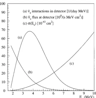
The pp process is the main contribution of solar neutrinos but the maximum energy of these neutrinos makes them challenging to detect on Earth. Neutrinos can also be created through the four following processes, according to Figure 1.3:
p + e + p! d + ⌫e (pep) (1.18) 3 2He + p!42He + e++ ⌫e (hep) (1.19) 7 4Be + e !73Li + ⌫e 7Be (1.20) 8 5B!84Be⇤+ e++ ⌫e 8B (1.21)
The number of produced elements from reactions 1.17 to 1.21 gives us the expected shapes of the neutrino spectra. For the pep and7Beprocesses, one should expect a discrete neutrino
energy spectrum since there is two final products. A contrario, the pp, hep and 8Blead to
continuous spectra, as it is shown in Figure 1.4.
The CNO cycle is illustrated in Figure 1.3. It is also called Bethe-Weizsäcker cycle and provides neutrinos even if the processes involved are less dominant. Indeed, the pp chain dom-inates at temperatures below 15 ⇥ 106 K in stars with mass lower than around 1.3 M [17].
Since the temperature sensitivity is much larger for the CNO cycle than for the pp chain, the CNO cycle contributes to about only 1.5 % of the Sun luminosity [18].
*
Figure 1.3: The pp chain (left) and the CNO cycle (right) with the generated neutrinos in bold, from [11].
Figure 1.4: Solar neutrino energy spectrum adapted from [19] with the uncertain-ties from [20].
1.3.2 Chasing solar neutrinos
Radiochemical experiments
The solar neutrino anomaly started with the Homestake experiment in 1968. This experi-ment, led by R. Davis Jr., was looking for radioactive argon isotopes, 37Ar, produced by the
interaction of solar neutrinos, ⌫e, on stable chlore isotopes, 37Cl, through the reaction:
⌫e+37Cl!37Ar + e (1.22)
The apparatus consisted of a 6.1 m diameter for 14.6 m long cylindrical tank filled with 615 tons of tetrachloroethylene, C2Cl4, installed in the Homestake Gold Mine in South
Dakota. A 4200 m water equivalent overburden allowed the experiment to be protected from cosmic rays.
Every two months, an extraction by chemical methods of the produced37Arwas performed
and subsequently counted. R. Davis Jr. and his collaborators noticed very soon after the start of the experiment that the number of 37Arwas to low compared to the predictions [21].
This “surprise” gave birth to the solar neutrino anomaly, even if at that time, dependending on the Standard Solar Model (SSM) used, the observed and predicted fluxes could match. It allowed J.N. Bahcall to conclude at that time that these results “are not in obvious conflict with the theory of stellar structure” [22].
With more than 25 years of data, the Homestake experiment provided a37Arproduction
rate of 2.56 ± 0.16 (stat) ± 0.16 (syst) SNU5, about three times lower than the predictions [23].
Several tests were performed in order to verify that the detector was working properly, with-out finding any misbehavior.
Due to this huge discrepancy, other experiments started, such as the GALLEX6/GNO7
and SAGE8 experiments. The GALLEX/GNO experiment was located in the Laboratori
Nazionali del Gran Sasso (LNGS) in Italy. The SAGE experiment is placed in the Baksan Neutrino Observatory (BNO) in Russia. They are both based on a solar neutrino interaction on 71Ga instead of37Cl:
⌫e+71Ga!71Ge + e (1.23)
The GALLEX/GNO experiment used 100 tons of gallium chloride GaCl3, containing
about 30 tons of gallium whereas the SAGE experiment opted for about 50 tons of gallium in the form of a liquid metal. Whereas the Homestake experiment had a threshold at 814 keV, the gallium experiments had a lower threshold at 233 keV, allowing them to detect solar neutrinos from the pp reaction (1.17).
51 Solar Neutrino Unit = 1 interaction per 1036 target atoms per second
6GALLium EXperiment
7Gallium Neutrino Observatory
The produced 71Ge were extracted through chemical methods and their decay into 71Ga
was measured. After 10 years of running, about half of the expected signal was measured for both experiments [24, 25]:
69.3 ± 4.1 (stat) ± 3.6 (syst) SNU (GALLEX/GNO) (1.24)
70.8+5.3+3.75.2 3.2SNU (SAGE), (1.25)
instead of the 128+9
7 SNU expected from the BP00 SSM [26].
Various tests were also performed, such as the introduction of 51Cr sources in both
ex-periments. It was concluded that the deficit was not due to experimental artifacts [27, 28]. Water Čerenkov experiments
The Kamiokande9 and Super-Kamiokande experiments were also looking for solar neutrinos
in order to try to solve the anomaly on a non-radiochemical base. The solar neutrino detection relies on the Čerenkov light produced by the recoil of the electron in the elastic scattering (ES) reaction:
⌫↵+ e ! ⌫↵+ e (ES), (1.26)
where ↵ stands for e, µ or ⌧.
Even if this reaction is sensitive to all neutrino flavors, ⌫e elastic scattering dominates
because of a six time higher cross-section for ⌫e with respect to the ones for ⌫µ and ⌫⌧ [29].
The diffusion allowed to know the direction of the incoming neutrino, leading to the pos-sibility of discriminating between solar neutrino events and background events. Nevertheless, since these experiments were first designed to look for nucleon decay with energy of the or-der of 1 GeV, they were only sensitive to the highest neutrino energy spectrum components in Figure 1.4, i.e. 8B and hep components from reactions (1.19) and (1.21). A deficit was
confirmed for the 8B component, as shown in Table 1.1.
Deadlocked
At the dawn of the third millennium, the solar neutrino anomaly remained unsolved. Dif-ferent radiochemical experiments saw deficits as well as water Čerenkov experiments which used a complete different detection method. Table 1.1 illustrates where the physicists stood before the results from the SNO experiment.
Table 1.1: Solar neutrino flux, neutrino capture rate for 37Cl and 71Ga
experi-ments from the BP00 SSM [26] and measured flux and rate for the Homestake [23], GALLEX/GNO [24], SAGE [25] and Super-Kamiokande [30] experiments. Statis-tical and systematic uncertainties have been added in quadrature.
Process BP00 (cm 2s 1) RCl (SNU) RGa (SNU) SK (cm 2s 1)
pp 5.95 ⇥ 1010 - 69.7 -pep 1.40 ⇥ 108 0.22 2.8 -hep 9.3 ⇥ 103 0.04 0.1 < 73 ⇥ 103 7Be 4.77 ⇥ 109 1.15 34.2 -8B 5.05 ⇥ 106 5.76 12.1 (2.35 ± 0.08) ⇥ 106 13N 5.48 ⇥ 108 0.09 3.4 -15O 4.80 ⇥ 108 0.33 5.5 -17F 5.63 ⇥ 106 0.0 0.1 -Total 6.54 ⇥ 1010 7.6+1.3 1.1 128+97 -Homestake - 2.56 ± 0.23 -GALLEX/GNO - - 69.3 ± 5.5 SAGE - - 70.8+6.56.1
1.3.3 Solving the anomaly
One had to wait until 2002 and the results from the SNO experiment to be able to solve the solar neutrino anomaly [31]. Like Super-Kamiokande, SNO is a water Čerenkov experiment, sensible only to 8B and hep components. The detector consists of a 12 m diameter sphere
filled with an ultrapure heavy water (D2O), different from the Super-Kamiokande one which
is filled with ultrapure water (H2O). Due to this outline, SNO was sensitive in one hand to
the elastic scattering (ES) reaction, as Super-Kamiokande, and on another hand to the charge current (CC) reaction and to the neutral current (NC) reaction due to the interaction of the neutrinos on deuterium:
⌫e+ d! p + p + e (CC) (1.27)
⌫↵+ d! p + n + ⌫↵ (NC), (1.28)
where ↵ stands for e, µ or ⌧.
Whereas the charged current reaction is only sensitive to ⌫e, the neutral current reaction
is sensitive to all neutrino flavors. If there is no other neutrino flavor involved but ⌫e, then
the solar neutrino flux from the charge current reaction should be of the order of the one from the neutral current reaction. SNO succeeded in measuring both CC and NC:
CC = 1.76+0.060.05(stat)+0.090.09(syst) cm 2s 1 (1.29) NC= 5.09+0.440.43(stat)+0.460.43(syst) cm 2s 1 (1.30)
The total flux measured from the neutral current process is in agreement with the pre-dicted value from Table 1.1. One can observe a discrepency between the CC and NCvalues
which can be interpreted as a non-zero flux of ⌫µ and ⌫⌧ from the initial 8B neutrino flux.
With a change of variables, one can then deduce e and µ⌧:
e= 1.76+0.050.05(stat)+0.090.09(syst) cm 2s 1 (1.31) µ⌧ = 3.41+0.450.45(stat)+0.480.45(syst) cm 2s 1 (1.32)
With a non-electron neutrino flux 5.3 greater than zero, this results allowed to confirm that during their journey, some of the ⌫ecreated through the8Bprocess from reaction (1.21)
transformed themselves into another neutrino flavor, giving a deficit of ⌫e when looking only
for them on Earth.
Thanks to the use of the heavy water, the SNO experiment confirmed the reliability of the SSM prediction and solved the solar neutrino anomaly. Back in 1972, B. Pontecorvo sent a fax to J.N. Bahcall telling him [32]:
“It would be nice if all this will end with something unexpected from the point of view of particle physics. Unfortunately, it will not be easy to demonstrate this, even if nature works that way.”
The theory of neutrino oscillation was pointed out as the best way to resolve this anomaly. We will investigate in more details this theory in the next chapter.
1.4 Atmospheric neutrino anomaly
Atmospheric neutrinos are created from the interaction of primary cosmic rays with the Earth’s atmosphere. This process gives birth to a particle zoo which contains among them pions and kaons we have already seen in the description of the ⌫µdiscovery. Those pions and
kaons decay, producing muons and ⌫µ. Those muons also decay, producing ⌫e and ⌫µ. We
call atmospheric neutrinos the ⌫e and ⌫µ produced in these decays. One should expect then
to measure two ⌫µ for every ⌫e. It is in reality a bit more complicated but stays valid for
energies below 1 GeV.
Water Čerenkov experiments are looking for the leptons produced in the charge current quasi-elastic (CCQE) scattering of neutrinos in the detector, as well as single-pion and multi-pion production from both charged and neutral currents:
⌫l(¯⌫l) + X ! l (l+) + Y (CCQE) (1.33)
⌫l(¯⌫l) + X ! l (l+) + Y + ⇡+(⇡ ) (CC single-pion) (1.34)
⌫l(¯⌫l) + X ! ⌫l(¯⌫l) + X + ⇡0 (NC single-pion), (1.35)
The CCQE reaction is the dominant one for energies below 1 GeV. The strength of this kind of experiments is to easily discriminate between electron-like events and muons-like events by observing the Čerenkov rings which differs from one to another. It is then of interest to look for single-ring e-like and single-ring µ-like produced by the interaction of atmospheric neutrinos in the detector.
In 1988, the Kamiokande collaboration pointed out a deficit of ⌫µ when comparing with
the prediction, as it can be seen in Figure 1.5. If the number of recorded e-like events was 105 ± 11 % of the estimation, it was only 59 ± 7 % for µ-like events [33]. Even if a way to explain this deficit was that “the calculation of the atmospheric neutrino fluxes may not be correct”, this results brought a new interest and gave birth to what would be called the atmospheric neutrino anomaly.
Figure 1.5: Momentum distributions for (a) e-like events and (b) µ-like events, from [33].
Several other experiments started then to investigate this deficit. In 1992, with the analy-sis of 610 single-ring events recorded for a total exposure of 7.7 kton year, the IMB experiment confirmed a deficit by measuring a 0.36 ± 0.02 (stat) ± 0.02 (syst) fraction of µ-like events over all events when its simulation predicted a fraction of 0.51 ± 0.01 (stat) ± 0.05 (syst) [34]. In 1997, with the use of an iron tracking calorimeter, the Soudan 2 experiment confirmed also a deficit. After a total exposure of 1.52 kton year, the number of e-like events corresponded to 109± 21 % of the estimation whereas it corresponded only to 79 ± 18 % for µ-like events [35]. In order to study the ⌫µ/⌫e flux ratio, one can calculate the ratio-of-ratios R defined as:
R = (Nµ/Ne)Data (Nµ/Ne)MC
, (1.36)
where Nµ and Ne stand respectively for µ-like and e-like events.
If both data and prediction are in agreement, one should measure R = 1. In 1998, the Super-Kamiokande experiment reported R = 0.63 ± 0.03 (stat) ± 0.05 (syst), confirming here
again a deficit of µ-like events [36].
Since neutrinos interact very weakly, atmospheric neutrinos born on the other side of the Earth should easily cross it before interacting in a detector, leading to a flight path from 20 to 12000 km. Thanks to the Čerenkov light pattern, one can then reconstruct the lepton direction which, for energies above 1 GeV, is strongly correlated to the initial incoming direc-tion of the neutrino. The ratio of the number of upward to downward µ-like events has been measured by Super-Kamiokande to be 0.52+0.07
0.06(stat) ± 0.01 (syst) when one should expect
a value close to the unity. The same ratio for e-like events did not show any discrepancy, as it can be seen in Figure 1.6.
These misbehaviors for both the expected number of µ-like events and their angular distortion allowed the Super-Kamiokande collaboration to conclude [37]:
“While the zenith angle dependence of the µ-like data cannot be ex-plained by any plausible systematic detector effect considered, the rel-ative deficit of upward-going µ-like events from neutrinos that traveled a long distance suggests the disappearance of ⌫µ via neutrino
oscilla-tions.”
Figure 1.6: Zenithal angle distributions for fully contained single-ring e-like and single-ring µ-like events, from [38]. The points correspond to the data, the box histograms to the non-oscillation prediction and the lines to the best fit.
1.5 Unsolved anomalies
The solar and atmospheric neutrino anomalies were solved by considering a three neutrino oscillation framework, which will be reviewed in detail in the next chapter. The anomalies described in this section can not be solved through a three neutrino oscillation scenario. Up to now, they remain unsolved.
1.5.1 Reactor antineutrino anomaly
The Double Chooz experiment, which will be described in the third chapter, started taking data in April 2011 with only one detector. The final configuration implies two identical detec-tors located at different baselines from two nuclear reacdetec-tors, in order to get rid of systematic uncertainty coming mainly from the lack of precision of the ¯⌫espectra prediction. The reactor
flux error is about 1.8 %, which is the main source of uncertainty for Double Chooz without a second detector [39, 40, 41, 42].
In order to reduce this error, new calculations of the ¯⌫e spectra coming from235U,239Pu, 241Puand 238U were performed, revealing an underestimation of about 3 % [43]. A complete
re-analysis of all reactor experiments at reactor-detector distance lower than 100 m followed, leading to a change in the ratio R of observed event rate to predicted rate. Whereas this ratio was 0.976 ± 0.024 before, it changed to 0.943 ± 0.023 with the new calculations. This deviation from unity at 98.6 % C.L. is called the reactor antineutrino anomaly [44].
*
Figure 1.7: Ratio of the data to the non-oscillation prediction as a function of the distance (left) and sin2(2✓
13) (right), from [45].
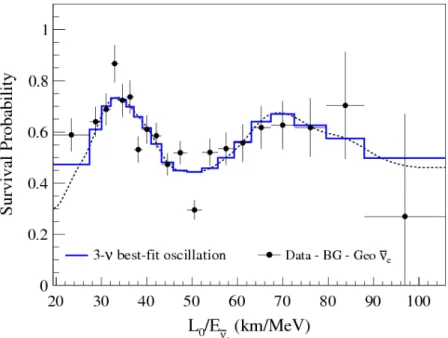
Recent investigations which included the precise measurement of the ✓13 mixing angle
confirmed the discrepency and determine R = 0.959 ± 0.009 (experiment uncertainty) ± 0.027 (flux systematics) [45]. Figure 1.7 shows the ratio of the data to the non-oscillation prediction as a function of the distance from the corresponding reactor core (left) and as a function of sin2(2✓
13) with and without its best fit value (right). It was pointed out that this
for an ¯⌫e to oscillate, at very short distance, into a hypothetical new neutrino state which
remains insensitive to the electroweak interaction.
1.5.2 GALLEX and SAGE, the gallium anomaly
While the solar neutrino anomaly was not yet solved, the radiochemical gallium experiments GALLEX and SAGE exposed their detector to intense calibration sources in order to check any misbehavior which could explain the solar neutrino deficit they observed. GALLEX used two intense 51Cr sources. The first one was deployed between June and October 1994 and
the second one between October 1995 and February 1996. The combined value of the ratio R between the neutrino source strength and the measured one was 0.93 ± 0.08, not enough to explain the solar neutrino deficit [27]. SAGE used also a 51Cr source and went to the same
conclusion [28]. SAGE decided later on to expose its detector to a 37Arsource. In this case,
R = 0.79+0.090.10, nearly 2.5 from unity [46].
Figure 1.8: Ratio of the data to the prediction for the radiochemical gallium experiments GALLEX and SAGE, from [46]. The hashed region corresponds to the weighted average.
An average value of the two different51Crcalibration campaigns from GALLEX together
with the 51Cr one and the 37Ar one from SAGE allowed to find a discrepency between the
prediction and the observation, as it can be seen in Figure 1.8 [46]:
“The weighted average value of R, the ratio of measured to predicted
71Ge production rates, is 0.88 ± 0.05, more than two standard
devi-ations less than unity. Although not statistically conclusive, the com-bination of these experiments suggests that the predicted rates may be overestimated.”
Another explanation comes from the possible ⌫e oscillation into a sterile neutrino state,
1.5.3 LSND and MiniBooNE anomalies
The LSND10 experiment took place at the Los Alamos Neutron Science Center from 1993 to
1998. This experiment was designed to study ¯⌫µ! ¯⌫e from µ+ decay at rest. A total excess
of 87.9 ± 22.4 ± 6.0 ¯⌫e events identified through IBD interactions were registered above
the expected background [47]. This excess can be interpreted as an oscillation, although the mass-squared difference reported stands in the range [0.2, 10 eV2], which does not correspond
to the mass-squared differences of solar or atmospheric neutrinos we will review in the next chapter. This observation implies the existence of at least one sterile neutrino with a mass greater than 0.4 eV.
The MiniBooNE11 experiment has been designed to investigate the LSND results. With
a similar L/E range, MiniBooNE has been studied both ¯⌫µ ! ¯⌫e and ⌫µ ! ⌫e transitions.
While the results for the ¯⌫µ ! ¯⌫e transition are fairly in agreement, the ⌫µ ! ⌫e transition
has been found to be inconsistent [48]. Figure 1.9 shows the energy spectra with and without background substraction for both antineutrino and neutrino modes. A fit analysis was per-formed on a two-neutrino oscillation model, which shows a different behavior for antineutrino and neutrino modes.
The excess in the ¯⌫µ ! ¯⌫e transition being localized in the low energy part of the
spec-trum, the MicroBooNE experiment has been designed to investigate this specific part of the energy spectrum.
10Liquid Scintillator Neutrino Detector
*
Figure 1.9: Energy spectra before (left) and after (right) background substraction for both antineutrino and neutrino modes, from [48]. Best fit for each mode as well as two fits with different sets of oscillation parameters are shown.
2
Deepening the neutrino
knowledge
There are two possible outcomes: if the result confirms the hypothesis, then you’ve made a measurement. If the result is contrary to the hypothesis, then you’ve made a discovery. Enrico Fermi
Contents
2.1 Neutrinos within the Standard Model . . . 24 2.1.1 Masses in the Standard Model: the Higgs mechanism . . . 25 2.2 Neutrino masses . . . 26 2.2.1 Dirac mass term . . . 26 2.2.2 Majorana mass term . . . 27 2.2.3 See-saw mechanism . . . 28 2.2.4 Neutrino masses from experiments . . . 29 2.3 Neutrino mixing and oscillation . . . 31 2.3.1 Neutrino mixing . . . 32 2.3.2 Neutrino oscillation . . . 32 2.3.3 Solar sector, m2 21 and ✓12 . . . 37 2.3.4 Atmospheric sector, m2 32 and ✓23 . . . 39 2.3.5 ✓13 sector . . . 39 2.4 Cosmological informations . . . 46 2.5 Sterile neutrinos? . . . 46
Our understanding of neutrinos is far from being complete. Although the neutrino oscil-lation theory is well established, throwing out the Standard Model requirement of a massless neutrinos, physicists have still to answer key questions, such as the nature of the neutrino itself, Dirac or Majorana, or its mass.
2.1 Neutrinos within the Standard Model
The Standard Model of particle physics is a quantum field theory which aims at unifying the strong, weak and electromagnetic interactions in order to marry quantum physics together with special relativity. It allows to describe elementary particles properties and interactions between them. It derives from the Fermi theory [3] together with the Glashow-Weinberg-Salam theory [49, 50].
The Standard Model is a gauge theory based on the SU(3)C⌦ SU(2)L⌦ U(1)Ylocal sym-metry group where C, L and Y denote repectively the color, the left-handed chirality and the weak hypercharge [11]. To each group corresponds a certain number of generators, the vector gauge bosons. SU(3)C owns eight generators, the gluons, which are also the force carriers of the strong interaction. SU(2)L⌦ U(1)Y owns four generators. The spontaneous breaking of
the SU(2)L⌦ U(1)Y symmetry through the Brout-Englert-Higgs mechanism allows to
gener-ate the masses of the W± and Z0 bosons, force carriers of the weak interaction [51, 52]. The
important mass they acquired during this process is responsible for the short range of the weak interaction. The photon, , is finally the force carrier of the electromagnetic interaction. Weak and electromagnetic interactions were unified thanks to the Glashow-Weinberg-Salam theory of electroweak interaction [49, 50], which was able to predict the W± and Z0 masses.
Table 2.1: Elementary properties of the fermions. Masses are taken from [29] for the quarks and charged leptons and from [53, 54, 55] for the upper limits on the masses of the neutrinos.
Fermions 1st family 2nd family 3rd family
Quarks
u (up) c(charm) t(top)
mu= 2.3+0.70.5 MeV mc = 1.275 ± 0.025 GeV mt= 173.5 ± 0.6 ± 0.8 GeV
d(down) s (strange) b(bottom)
md= 4.8+0.70.3 MeV ms= 95 ± 5 MeV mb= 4.18 ± 0.03 GeV
Leptons
e µ ⌧
me= 0.511MeV mµ= 105.658MeV m⌧ = 1.777GeV
⌫e ⌫µ ⌫⌧
m⌫e < 2.05eV m⌫µ < 170keV m⌫⌧ < 18.2 MeV
The Standard Model describes the fermions, which are the components of the matter, as well as the bosons, which are the force carriers. Whereas the fermions own half-integer spins, obey the Fermi-Dirac statistics and follow the Pauli exclusion principle, the bosons own integer spin and obey the Bose-Einstein statistics. The fermions can be divided into two sub-categories, the quarks and the leptons. There are three families of quarks and leptons, as it can be seen in Table 2.1. Quarks are subject to the four fundamental interactions which are the strong, weak, electromagnetism and gravitational interactions. They can not be observed directly since they are confined into hadrons, such as baryons when they are arranged with
three quarks or mesons when they form a quark/antiquark pair. Leptons do not interact through the strong interaction but are subject to the three other fundamental interactions, except for the neutrinos which do not interact through the electromagnetic interaction. The left-handed charged lepton together with the left-handed neutrino form a doublet of SU(2)L. Whereas the right-handed charged lepton exists, the right-handed neutrino is not considered in the Standard Model. Up to now, there is not yet an experimental evidence for a right-handed neutrino.
2.1.1 Masses in the Standard Model: the Higgs mechanism
The masses of bosons and fermions are generated through the Higgs mechanism. The in-troduction of a complex scalar field (x) allows to generate masses through spontaneous symmetry breaking. This field can be written through the Higgs doublet:
(x)⌘
+(x)
0(x)
!
, (2.1)
where +(x)and 0(x)are respectively the charged and neutral complex scalar fields.
The general potential associated to this Higgs field is given by: V ( ) = µ2 † + ( † )2= ✓ † +µ2 2 ◆2 µ4 4 (2.2)
Neglecting the µ4/4 constant term, this potential has a minimum for † = µ2/2 . In
order to have the spontaneous symmetry breaking, we have to consider µ2 < 0. The minimum
of this potential corresponds to the vacuum. The vacuum expactation value, h i, is due to the neutral complex scalar field, 0, and can be expressed as:
h i = p1 2 0 v ! with v⌘ r µ2 (2.3) The mass of the BEH1 boson, sometimes simply called Higgs boson, is linked to v through:
mBEH =p2 v2 =p 2µ2, (2.4)
which can not be predicted by the Standard Model since µ2 has been introduced without
being connected to other measurable quantities.
The existence of this boson was first postulated in 1964 by F. Englert and R. Brout and independently by P.W. Higgs [51, 52]. On July 4, 2012, the two main LHC2 experiments,
ATLAS and CMS, announced its discovery, giving the Nobel Prize the next year to P.W. Higgs and F. Englert3 [56, 57].
1Brout-Englert-Higgs
2Large Hadron Collider
The Standard Model does not provide neither a right-handed neutrino nor a mass for the neutrino. Nevertheless, it is still possible to add an extension to this model in order to give masses to the neutrinos.
2.2 Neutrino masses
The mass term arises from the Lagrangian of interaction of leptons and Higgs bosons when the symmetry is spontaneously broken [58]. It allows to connect a field to its conjugate ¯, leading to the Lagrangian density:
L = m ¯ (2.5)
The field can be decomposed into a “left-handed” field, L, and a “right-handed” field, R, such that:
= L+ R (2.6)
Land Rare linked to the notions of chirality and helicity. When considering relativistic
particles, the chirality almost coincides with the projection of its spin on its momentum, i.e. its helicity. The chirality projector PLand PRact on such that:
L= PL R= PR , (2.7)
with the following properties:
PL2 = PL PR2 = PR PLPR= PRPL= 0 PL+ PR= 1 (2.8)
Let us now have a look at the charge conjugation operator C. This operator allows to change a particle into its antiparticle:
C
! c=C ¯T (2.9)
Acting on chiral fields and neglecting phase factors, this operator allows to change a left-handed field into a right-handed field, and vice versa:
L! C Lc =C ¯LT ⌘ R R ! C Rc =C ¯TR⌘ L (2.10)
The field from equation (2.6) can then be expressed in this way:
= L+ cL (2.11)
2.2.1 Dirac mass term
We build a neutrino Dirac mass term by introducing the decomposed field from equation (2.6) into the Lagrangian density from equation (2.5):
LD = M
D(¯⌫L+ ¯⌫R)(⌫L+ ⌫R)
= MD(¯⌫L⌫R+ ¯⌫R⌫L)
where the terms ¯⌫L⌫L and ¯⌫R⌫R vanish due to the chirality projector properties from
equa-tions (2.8): ¯
⌫L⌫L= ⌫L† 0⌫L= ⌫L† 0PL⌫ = ⌫L†PR 0⌫ = (PR⌫L)† 0⌫ = (PRPL⌫)† 0⌫ = 0, (2.13)
where 0 corresponds to one of the four Dirac matrices.
The Dirac mass term considers both the left-handed and right-handed fields. Neverthe-less, the right-handed field does not participate to any Standard Model interaction. It can be removed by using a Majorana mass term.
2.2.2 Majorana mass term
Since the left-handed field is linked to the right-handed field through the charge conjugation, we can build a neutrino Majorana mass term for the ⌫L field only. This neutrino Majorana
mass term can be obtained by injecting equation (2.11) into equation (2.5): LM= 1 2ML(⌫L+ ⌫ c L)(⌫L+ ⌫Lc) = 1 2ML(⌫L⌫ c L+ ⌫Lc⌫L) = 1 2ML⌫ c L⌫L+h.c. (2.14)
Using equation (2.10), one can express ⌫c
L in terms of ⌫L: ⌫c L= (C⌫LT)† 0= ⌫LT( 0)TC† 0= ⌫LTC†, (2.15) leading to: LM= 1 2ML⌫ T LC†⌫L+h.c. (2.16)
Nevertheless, it is also possible to add a Majorana mass term for the ⌫Rfield. The general
neutrino Majorana mass term can then be expressed as: LM= 1 2ML⌫ T LC†⌫L+ 1 2MR⌫ T RC†⌫R+h.c. (2.17)
One can directly observe from equation (2.11) that = c or, in other words, that a
Majorana particle is its own antiparticle [59]. A charged particle can not therefore be a Ma-jorana particle, only neutrino can be.
Neutrinoless double decay experiments are still investigating whether the neutrino is a Majorana particle, we will talk about these experiments later on in this chapter.
2.2.3 See-saw mechanism
Let us now consider the most general neutrino mass term by combining both Dirac and Majorana mass terms. It leads to the Lagrangian density:
LD+M = 1 2ML⌫ T LC†⌫L MD⌫¯R⌫L+ 1 2MR⌫ T RC†⌫R+h.c. (2.18)
LD+M can also be written in a more compact way:
LD+M = 1
2N
T
LC†MNL+h.c., (2.19)
with NL defined as:
NL= ⌫L ⌫c R ! (2.20) Since MD is a non-diagonal matrix and ML and MR have to be symmetric, M can be
expressed as:
M = ML MD
MDT MR
!
(2.21) M can then be diagonalized using an orthogonal matrix U such that:
D = UTMU = m1 0 0 m2
!
(2.22) Playing with the traces and the determinants of these two matrices, we end with a system with two unknowns that one can easily solve in order to find the values of the neutrino mass eigenvalues m1 and m2: m2,1= ML+ MR 2 ± s✓ ML MR 2 ◆2 + M2 D (2.23)
From this general case, we can build the so-called “see-saw” mechanism. This mechanism allows to explain why the “active” neutrinos are so light by compensating with heavy neutri-nos, called “sterile” since they can not interact through the weak interaction of the Standard Model. This mechanism assumes therefore the existence of a sterile neutrino through a min-imal extension of the Standard Model. From the neutrino mass eigenvalues m1 and m2 we
have calculated earlier, m1 < m2. Assuming MR MD and ML= 0, we are left with:
m1'
M2
D
MR
m2' MR (2.24)
The negative sign of m1 can be removed by taking the physical neutrino field through the
action of the 5 matrix [60]. Considering MD to be a quark or charged lepton mass, we end
with:
m1⇥ m2= MD2 (2.25)
This corresponds to the see-saw relation. It tells us that if an active neutrino of mass m1
2.2.4 Neutrino masses from experiments
decay experiments
As we have already seen in the previous chapter, the decay is a radioactivity process in which an electron and an ¯⌫e are emitted, according to the reaction:
A
ZX!Z+1AY + e + ¯⌫e (2.26)
When neglecting the A
Z+1Y recoil, the electron and the ¯⌫e share the available energy. In
the case of a massless neutrino, the electron spectrum would extend up to the maximum available energy Emax
e = E0. A contrario, if the neutrino has a mass, then the electron
en-ergy spectrum will be distorted since Emax
e will no longer be equal to E0. We will have in
this case Emax
e = E0 m⌫e, as it is shown in Figure 2.1. This kind of investigation does not
rely on the nature of the neutrino, i.e. Dirac or Majorana.
Figure 2.1: The electron energy spectrum of tritium decay (a) with a narrow region around the endpoint (b), from [61].
The Mainz, Troitsk and upcoming KATRIN experiments are based on the tritium decay spectroscopy. One needs a low endpoint since the neutrino mass expected is low. With an endpoint at 18.6 keV, a simple electronic shell and a half life of 12.3 years, the tritium is a good candidate.
The Mainz experiment reported in 2005 an upper limit of m⌫e 2.3 eV at 95 % C.L. [62]
and the Troitsk experiment an upper limit of m⌫e 2.12 eV with a Bayesian approach and
m⌫e 2.05 eV with a Feldman and Cousins approach [53, 63]. The KATRIN experiment is
still under construction and would have an estimated sensitivity of m⌫e = 0.35 eV at 90 %
C.L., which is about one order of magnitude better than the previous experiments [61]. Limits were also obtained on the effective ⌫µ and ⌫⌧ masses, although less stringent.
An upper limit on m⌫µ was determined by studying the decay of pions in the reaction
⇡+ ! µ++ ⌫µ, leading to m⌫µ < 170 keV [54]. Upper limit on m⌫⌧ was derived by
study-ing the decay of taus in the reactions ⌧ ! 2⇡ ⇡+⌫
⌧ and ⌧ ! 3⇡ 2⇡+(⇡0)⌫⌧, leading to


![Table 2.1: Elementary properties of the fermions. Masses are taken from [29] for the quarks and charged leptons and from [53, 54, 55] for the upper limits on the masses of the neutrinos.](https://thumb-eu.123doks.com/thumbv2/123doknet/2318543.28470/39.892.98.768.664.899/table-elementary-properties-fermions-masses-charged-leptons-neutrinos.webp)
![Figure 2.3: Values of the three neutrino mass eigenstates as a function of the light- light-est eigenstate when considering a normal hierarchy (left) or an inverted hierarchy (right), from [74].](https://thumb-eu.123doks.com/thumbv2/123doknet/2318543.28470/50.892.138.785.129.430/neutrino-eigenstates-function-eigenstate-considering-hierarchy-inverted-hierarchy.webp)