DOI:10.1051/0004-6361/201220529
c
ESO 2013
Astrophysics
&
The 2.35 year itch of Cygnus OB2 #9
II. Radio monitoring
?,??R. Blomme
1, Y. Nazé
2,???, D. Volpi
1, M. De Becker
2, R. K. Prinja
3, J. M. Pittard
4, E. R. Parkin
5, and O. Absil
21 Royal Observatory of Belgium, Ringlaan 3, 1180 Brussels, Belgium e-mail: Ronny.Blomme@oma.be
2 Département AGO, Université de Liège, Allée du 6 Août 17, Bât. B5C, 4000 Liège, Belgium
3 Department of Physics & Astronomy, University College London, Gower Street, London WC1E 6BT, UK 4 School of Physics and Astronomy, The University of Leeds, Woodhouse Lane, Leeds LS2 9JT, UK 5 Research School of Astronomy and Astrophysics, The Australian National University, Australia Received 10 October 2012/ Accepted 7 December 2012
ABSTRACT
Context.Cyg OB2 #9 is one of a small set of non-thermal radio emitting massive O-star binaries. The non-thermal radiation is due to synchrotron emission in the colliding-wind region. Cyg OB2 #9 has only recently been discovered to be a binary system, and a multi-wavelength campaign was organized to study its 2011 periastron passage.
Aims.We want to better determine the parameters of this system and model the wind-wind collision. This will lead to a better understanding of the Fermi mechanism that accelerates electrons up to relativistic speeds in shocks and its occurrence in colliding-wind binaries. We report here on the results of the radio observations obtained in the monitoring campaign and present a simple model to interpret the data.
Methods.We used the Expanded Very Large Array (EVLA) radio interferometer to obtain 6 cm and 20 cm continuum fluxes during the Cyg OB2 #9 periastron passage in 2011. We introduce a simple model to solve the radiative transfer in the stellar winds and the colliding-wind region, and thus determine the expected behaviour of the radio light curve.
Results.The observed radio light curve shows a steep drop in flux sometime before periastron. The fluxes drop to a level that is comparable to the expected free-free emission from the stellar winds, suggesting that the non-thermal emitting region is completely hidden at that time. After periastron passage, the fluxes slowly increase. We use the asymmetry of the light curve to show that the primary has the stronger wind. This is somewhat unexpected if we use the astrophysical parameters based on theoretical calibrations. But it becomes entirely feasible if we take into account that a given spectral type-luminosity class combination covers a range of astrophysical parameters. The colliding-wind region also contributes to the free-free emission, which can help explain the high values of the spectral index seen after periastron passage. Combining our data with older Very Large Array (VLA) data allows us to derive a period P= 860.0 ± 3.7 days for this system. With this period, we update the orbital parameters that were derived in the first paper of this series.
Conclusions.A simple model introduced to explain only the radio data already allows some constraints to be put on the parameters of this binary system. Future, more sophisticated, modelling that will also include optical, X-ray, and interferometric information will provide even better constraints.
Key words.stars: individual: Cyg OB2 #9 – stars: early-type – stars: mass-loss – radiation mechanisms: non-thermal – acceleration of particles – radio continuum: stars
1. Introduction
Among the early-type stars there are a number of non-thermal radio emitters. It is now generally accepted that all such stars are colliding-wind binaries (Dougherty & Williams 2000; De Becker 2007;Blomme 2011). In a massive early-type binary the strong winds from both components collide, leading to the formation of two shocks, one on each side of the contact dis-continuity where the two winds collide. Around those shocks a fraction of the electrons is accelerated up to relativistic speeds. This is believed to be due to the Fermi acceleration mechanism ? Based on observations with the Expanded Very Large Array (EVLA), which is operated by the National Radio Astronomy Observatory. The National Radio Astronomy Observatory is a facility of the National Science Foundation operated under cooperative agree-ment by Associated Universities, Inc.
?? Figure 1 is available in electronic form at http://www.aanda.org
??? Research Associate FRS-FNRS.
(Eichler & Usov 1993). As these electrons spiral around in the magnetic field, they emit synchrotron radiation, which we detect as non-thermal radio emission. In addition, the hot compressed material in the colliding-wind region (CWR) also emits X-rays (Stevens et al. 1992;Pittard & Parkin 2010) and influences the shape of the optical spectral lines (Rauw et al. 2005).
While the general outline of the explanation for non-thermal radio emission is clear, there are still problems when detailed modelling of specific systems is attempted. In modelling the ra-dio flux variations of the short-period variable Cyg OB2 #8A, Blomme et al.(2010) failed to obtain the correct spectral index. For the well-observed WR+O binary WR 140, models fail to ex-plain the behaviour of the radio light curve (Williams et al. 1990; White & Becker 1995;Pittard 2011). Part of the problem is the difficulty in calculating all the effects of the Fermi acceleration ab initio. Another complication is the presence of clumping or porosity in the stellar winds of massive stars, making the esti-mates of mass-loss rates uncertain. As an added difficulty, the degree of clumping depends on the radius (Puls et al. 2006).
More detailed observations that will help constrain theoreti-cal models are therefore most important. To that purpose a multi-wavelength campaign was started (PI: Y. Nazé) to monitor the 2011 periastron passage of Cyg OB2 #9. That Cyg OB2 #9 is a binary was only discovered relatively recently. The system consists of an O5-5.5If primary and an O3-4III secondary in a highly eccentric (e ≈ 0.7) orbit with a period of ∼2.35 yr (Nazé et al. 2008;van Loo et al. 2008). Since its discovery as a binary, Cyg OB2 #9 has passed periastron twice. The 2009 passage was unobservable because it occurred when the system was in con-junction with the Sun. The 2011 periastron passage is therefore the first one that could be observed well.
In Nazé et al. (2012, hereafter Paper I) we presented the results from the optical and X-ray monitoring campaign. The CWR was detected in Hα, where it creates enhanced absorption and emission. Owing to the hot material in the CWR, the X-rays show phase-locked behaviour with the flux peaking at perias-tron. They indicate an adiabatic wind-wind collision for most of the time with the flux following the predicted inverse relation with the separation between the two components. Only close to periastron could the shock be turning radiative. The present pa-per is the second in the series, analysing the radio observations made by the Expanded Very Large Array (EVLA;Perley et al. 2011). Future papers will discuss the optical interferometry and the modelling of the system.
The non-thermal nature of Cyg OB2 #9 became clear from its high brightness temperature, its non-thermal spectral index, and its variability (White & Becker 1983;Abbott et al. 1984; Bieging et al. 1989; Phillips & Titus 1990). In a series of pa-pers, van Loo et al. (2004, 2005, 2006) tried to explain the non-thermal radio emission by a single star (the binary na-ture of this star was not yet known at that time). In a single star, it is assumed that the shocks due to the intrinsic insta-bility of the radiation driving mechanism are responsible for the Fermi acceleration (White 1985). However, the increasingly more sophisticated models used by van Loo et al. have failed to explain the observations.
A large set of VLA archive data allowed van Loo et al. (2008) to find a ∼2.35 yr period in the fluxes, strongly suggest-ing binarity. Simultaneously,Nazé et al.(2008) detected the bi-narity from optical spectroscopy. The orbital information was then refined further using additional optical spectra (Nazé et al. 2010; Paper I). Further evidence for the non-thermal nature of Cyg OB2 #9 comes from Very Large Baseline Array (VLBA) radio observations that clearly show the bow-shaped extended emission typical of a CWR in a binary system (Dougherty & Pittard 2006).
In this paper, we present the EVLA radio observations that were obtained as part of the 2011 Cyg OB2 #9 monitoring cam-paign. We derive the orbital period from these data. We also in-troduce a simple numerical model to help us interpret the obser-vations. In Sect. 2 we describe the data reduction of the radio observations. In Sect.3, we present the radio light curve and de-rive the binary period. In Sect.4we introduce a simple model, which we use in Sect.5to analyse and discuss the results, and Sect.6summarizes our findings and presents our conclusions.
2. Observations
2.1. EVLA data
Cyg OB2 #9 was monitored with the EVLA during the period January to August 2011. The observations (programme 10C-134) were obtained through the open shared risk observing
(OSRO) programme. Eleven observations were made, each time in C-band (4.832–5.086 GHz, 6 cm) and L-band (1.264−1.518 GHz, 20 cm). The observing log is given in Table1. During the monitoring period, the configuration of the EVLA changed from CnB (giving a lower spatial resolution) to A (the highest spatial resolution).
Each band is covered by 2 × 64 channels, each of 2 MHz width. To calibrate out instrumental and atmospheric effects, the phase calibrator J2007+4029 was used. An observation con-sisted of a phase calibrator – target – phase calibrator sequence, first in C-band, then in L-band. This sequence was followed by an observation of the flux calibrator (J0542+498=3C 147) in L and C band. The flux calibrator also serves as the bandpass calibrator. Time on target for a single observation is 5 min for C-band and 7 min for L-band.
2.2. Data reduction
The data were reduced using the Common Astronomy Software Applications1 (CASA) version 3.3.0 data reduction package.
The system already flags a number of problematic data (due to focus problems, incorrect subreflector position, off-source an-tenna position, or missing anan-tennas), and other flags are applied while reading in the data (shadowing by antennas). Careful at-tention was given to radio frequency interference (RFI). The small amount of RFI present in the C-band is removed by flag-ging the visibilities in the relevant channels. For the stronger and more extended RFI in L-band, we applied Hanning smoothing to remove the Gibbs ringing; after that the channels affected by the RFI were flagged.
The calibration sequence starts by assigning the correct flux to the flux calibrator (3C 147), using a model to take into ac-count that this source is slightly resolved. A preliminary gain phase calibration was applied before the delay and bandpass cal-ibration. This was followed by the final gain phase and gain am-plitude calibrations. The fluxscale was then transferred from the flux to the phase calibrator (J2007+4029). The phase calibrator fluxes are listed in Table1: they show the slow flux variations typical of many phase calibrators. The calibrations are then ap-plied to the flux and phase calibrators, as well as to the target. The calibrated data for flux and phase calibrators were inspected visually: if discrepant data were found, they were flagged and the calibration redone.
In L-band (20 cm), the phase calibrator is influenced by the radio galaxy Cyg A, which contributes about 0.05–0.5 Jy (de-pending on the configuration of the EVLA) to the image, while the phase calibrator itself is about 3 Jy. Since the sidelobes of such a strong source can influence the phase calibrator, we ap-plied self-calibration to improve the gain phases. The visibilities were then inspected and any discrepant data flagged.
In the next step an image was made from the target visibili-ties. For the C-band, this image covers an area somewhat larger than the primary beam (which is 170diameter). To gain comput-ing time, we make the image in the L-band somewhat smaller than the primary beam (which is 600diameter). The size of each (square) pixel was chosen such that it oversamples the synthe-sized beam by a factor of at least 4 in each dimension. The image is cleaned down to a level where the noise in the cen-tre is compatible with the expected noise. Images taken in the low-spatial resolution EVLA configurations contain substantial, extended Galactic background. This was removed by excluding the data on the shortest baselines during the imaging. A strong 1 http://casa.nrao.edu/
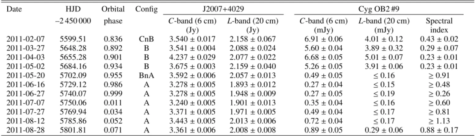
Table 1. Observing log, radio fluxes and spectral indexes of the EVLA data on Cyg OB2 #9.
Date HJD Orbital Config J2007+4029 Cyg OB2 #9
–2 450 000 phase C-band (6 cm) L-band (20 cm) C-band (6 cm) L-band (20 cm) Spectral
(Jy) (Jy) (mJy) (mJy) index
2011-02-07 5599.51 0.836 CnB 3.540 ± 0.017 2.158 ± 0.067 6.91 ± 0.06 4.01 ± 0.12 0.43 ± 0.02 2011-03-27 5648.28 0.892 B 3.541 ± 0.004 2.088 ± 0.024 5.60 ± 0.04 3.89 ± 0.32 0.29 ± 0.07 2011-04-03 5655.28 0.901 B 4.237 ± 0.029 2.077 ± 0.022 6.68 ± 0.05 5.01 ± 0.07 0.23 ± 0.01 2011-05-02 5684.16 0.934 B 3.675 ± 0.003 2.159 ± 0.040 5.26 ± 0.05 3.91 ± 0.06 0.23 ± 0.01 2011-05-20 5702.09 0.955 BnA 3.592 ± 0.006 2.057 ± 0.013 0.49 ± 0.05 ≤ 0.16 ≥ 0.91 2011-06-16 5729.12 0.986 A 3.278 ± 0.005 1.893 ± 0.012 0.27 ± 0.04 ≤ 0.15 ≥ 0.48 2011-06-27 5740.07 0.999 A 3.278 ± 0.005 1.948 ± 0.009 0.27 ± 0.05 ≤ 0.19 ≥ 0.26 2011-07-07 5750.06 0.011 A 3.240 ± 0.005 1.901 ± 0.013 0.35 ± 0.04 ≤ 0.16 ≥ 0.60 2011-07-27 5769.94 0.034 A 3.371 ± 0.005 1.971 ± 0.005 0.49 ± 0.04 ≤ 0.17 ≥ 0.81 2011-08-12 5785.86 0.052 A 3.443 ± 0.005 2.013 ± 0.006 0.72 ± 0.04 ≤ 0.17 ≥ 1.13 2011-08-28 5801.81 0.071 A 3.361 ± 0.006 2.008 ± 0.008 0.89 ± 0.05 0.29 ± 0.06 0.88 ± 0.17
Notes. We list observing date, heliocentric Julian date, orbital phase (using the Sect.3.2value for the period) and configuration of the EVLA. The fluxes of the phase calibrator J2007+4029 are listed next (at 6 and 20 cm), followed by the 6 and 20 cm fluxes of Cyg OB2 #9 and their spectral index. All fluxes have been calibrated on the flux calibrator 3C 147.
advantage of the present EVLA data over older VLA contin-uum data is that the many channels allow a sharp image further away from the field centre. To avoid introducing artefacts in such wide-field imaging (Bhatnagar et al. 2008), we needed to use the specific wide-field options in the CASA cleaning procedure. To handle the smaller-scale extended emission still present in the L-band images, the multi-scale option in the CASA clean proce-dure was used, with scales chosen to be 5, 10, 20, and 40 times the pixel size. For those images where the Cyg OB2 #9 flux was high enough (>∼1 mJy), we also applied a single round of phase-only self-calibration (further rounds of self-calibration no longer improve the image).
Two of our observations in the L-band (20 cm) are strongly affected by flaring from Cyg X-3 (which is within the primary beam). This microquasar consists of a Wolf-Rayet star and a compact object (most likely a black hole), and shows frequent and strong flaring activity. The Cyg X-3 multi-wavelength mon-itoring campaign reported byCorbel et al.(2012) shows a sharp transition from a quenched state to a major flare, with an onset estimated at MJD 55641.0±0.5 (i.e. March 21). On our March 27 observation, Cyg X-3 has a flux of ∼10 Jy; on the April 03 ob-servation this has decreased to ∼1 Jy, and on the May 02 obser-vation it has dropped down further to ∼0.07 Jy. This behaviour is compatible with theCorbel et al.monitoring results. Because of the decreasing sensitivity away from the field centre, the con-tribution of Cyg X-3 to our observations is a factor ∼3 less than the numbers given above. Nevertheless, for the March 27 and April 03 observations, the sidelobes of Cyg X-3 strongly perturb the cleaning of the image and the measurement of Cyg OB2 #9, which has a flux that is only a few mJy at best. The effect of the Cyg X-3 sidelobes on earlier and later observations is negligible. For the two most affected observations, we therefore first made an image, limiting the clean components to a small box around Cyg X-3. We used multi-frequency synthesis, result-ing in two images, one with the flux (averaged over the fre-quency band) and another with the spectral index. We then self-calibrated these images using one step of phase-only calibration, followed by one step of amplitude and phase calibration. The clean components of the Cyg X-3 image were then subtracted from the visibility data of the target. These data were then pro-cessed in the standard way to make an image and measure the fluxes. The procedure was very successful for the April 03 ob-servation, but in the March 27 observation important residual
effects of Cyg X-3 remain. In cleaning the latter image, we there-fore do not attain the expected noise level. We did not apply self-calibration to this image either.
For all images resulting from our dataset, we then deter-mined the flux and its corresponding error bar by fitting an ellip-tical Gaussian to the target. To measure the Cyg OB2 #9 flux, we fixed the size and position angle of the beam to the values of the synthesized beam (which is the shape that a point source should have after cleaning the image). In a number of L-band (20 cm) observations, Cyg OB2 #9 is not detected. In such cases, we as-signed an upper limit of three times the root-mean-square (rms) noise measured around the target position.
From the fluxes at 6 cm and 20 cm, we derive the spectral index α, given by Fν ∝να. The error bar on α is derived from standard error propagation, using the error bars on each of the fluxes. Where the 20 cm flux has an upper limit, only a lower limit for α can be determined.
3. Results
3.1. Radio light curve
Figure 1 shows contour plots of a small region around Cyg OB2 #9 for each of the 11 observations, at both 6 cm and 20 cm. The 6 cm images show a clear decrease in the flux with time, with a slight increase again towards the end of the series. The 20 cm series mirrors that behaviour, with the star being un-detectable from May 20 to August 12. The changing sizes of the synthesized beam reflect the changes of the EVLA antenna con-figuration. Although we know that Cyg OB2 #9 is a colliding-wind binary, the EVLA data do not allow us to resolve the CWR. Our resolution is at best ∼0.500(at 6 cm), but the VLBA data of Dougherty & Pittard(2006) show that the CWR has a size of ∼0.01500(at 3.6 cm).
The March 27 20 cm observation is of lesser quality, owing to the strong influence of Cyg X-3 on these data (see Sect.2.2). Our data reduction procedure manages to remove the strongest effects of Cyg X-3, but the quality of the data does not allow us to make an image with a sufficiently high dynamic range.
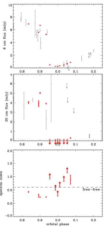
The measured Cyg OB2 #9 fluxes, their error bars and the spectral indexes are listed in Table1. Figure2 plots them as a function of orbital phase, with phase= 0.0 corresponding to pe-riastron. The epoch of periastron passage and the period were
Fig. 2.Radio fluxes and spectral indexes around the periastron passage of Cyg OB2 #9, as a function of orbital phase. The top figure shows the 6 cm flux, the middle one the 20 cm flux, and the bottom one the spectral index. The older VLA data fromvan Loo et al.(2008) are plotted with a grey line. The new EVLA data are shown with the thicker solid red line. The length of the line indicates the 1σ error bar on the flux. For the non-detections, upper limits are shown that are 3× the rms noise in the centre of the image. The fluxes have an additional uncertainty of ∼5% due to the absolute flux calibration (not shown on the figure). On the spectral index figure, the dashed line indicates the value for free-free emission (α= +0.6). Periastron occurs at phase = 0.0.
taken from this paper (see Sect. 3.2). The comparison with the older 6 cm VLA data from van Loo et al.(2008) shows good agreement, showing that the behaviour of Cyg OB2 #9 repeats very well over a number of orbital cycles. Although each of our data points is based on only 5–7 min on-target time, the quality
of these EVLA data is clearly much better than that of the older observations. For the values in the high-flux regime, the main uncertainty is due to the absolute flux calibration (estimated to be at the ∼5% level), not to the noise. For the 20 cm data the agreement is also good, though less constraining because of the large error bars and high upper limits of the older VLA data set. The new data show a steep drop in flux (both at 6 and 20 cm) between the May 02 and May 20 observations, corresponding to phases 0.934–0.955. Before that time, the 6 cm fluxes were in a high-flux regime, but with the flux slowly decreasing. The corresponding 20 cm fluxes are relatively constant during that time. The slight increase in the 20 cm flux between March 27 and April 03 (phase 0.892–0.901) could be due to problems with the data reduction (see Sect.2.2), but this is less likely for the 6 cm increase.
After the drop in flux, there is still a slight decrease in the 6 cm flux, just up to periastron passage. After periastron the flux starts to slowly increase again. The older VLA data at later phases connect very well with the new data points, also in this low-flux regime. At 20 cm the fluxes are so low that Cyg OB2 #9 is not detected. Only the last data point we have (August 28, phase 0.071) shows a detectable but low flux. Again the new data connect well with the increasing 20 cm flux shown in the older VLA data.
Previously, little information was available about the spec-tral index (α) and its changes in Cyg OB2 #9 (van Loo et al. 2008). The present data provide interesting information of the important changes of α during periastron passage (Fig.2, bottom panel). Before periastron, α goes down from 0.43 to 0.23. Since this is well below the+0.6 value expected for free-free emis-sion, it clearly shows the presence of a non-thermal component. From the May 20 (phase 0.955) observation onwards, the index increases; at times, even the lower limit indicates a value for free-free emission for a spherically symmetric wind, or an even higher value.
One would expect the synchrotron emission from the rela-tivistic electrons in the CWR to reach its maximum close to pe-riastron, where the stellar separation is smallest and the local magnetic field strongest. However, the observed situation here is almost the reverse. Both the drop in flux and the rise in spec-tral index point to a significant impact of free-free absorption on the synchrotron emission component by the stellar wind material close to periastron passage. This fact emphasizes the importance of orientation effects in the light curve of colliding-wind bina-ries, notably in the radio domain.
3.2. Period
The new EVLA data, in combination with the older VLA data (van Loo et al. 2008) cover a time span of ∼30 years, which is substantially longer than the time span covered by the optical spectroscopy (Paper I). The radio data are thus more suitable to deriving the orbital period of Cyg OB2 #9.
As invan Loo et al.(2008), we used the string-length method (Dworetsky 1983) to determine the period that best fits the data. We limited ourselves to the 6 cm observations, since the cov-erage at other wavelengths is sparser, and we exclude upper limits. We normalized the fluxes to the maximum flux over the combined VLA and EVLA dataset. This maximum is 8.5 mJy (VLA observation on 1984 November 27). The flux normaliza-tion introduces a good balance between phase difference and flux difference in the string-length calculation.
Intrinsically, the string-length method does not provide any error bar on its result. To determine the error bar, we applied
Table 2. Orbital solution for Cyg OB2 #9. Parameter Value P(d) – this paper 860.0 ± 3.7 T0 4020.72 ± 2.55 e 0.710 ± 0.016 ω1(◦) 191.9 ± 2.9 M1/M2 1.13 ± 0.08 γ1(km s−1) −33.9 ± 2.7 γ2(km s−1) 1.0 ± 2.8 K1(km s−1) 61.1 ± 3.0 K2(km s−1) 68.9 ± 3.4 a1sin i (R ) 730.1 ± 39.8 a2sin i (R ) 823.2 ± 44.9
Notes. Based on the period derived in Sect.3.2and the optical spectra fromPaper I. The present table supersedes the values given inPaper I. T0corresponds to periastron passage, in HJD−2 450 000.
the bootstrap technique. We made 5000 Monte-Carlo simula-tions, where we randomly choose a set of n data points out of the existing n observations (with replacement). We then applied the above string-length method, each time exploring 10 000 pe-riods between 750 and 950 days. We thus end up with a set of 5000 period determinations from which we can derive the best value and the error bar. For the best value, we used the median, and for the error bar we used quantiles to select the middle range that contains 68.3% of the values (this corresponds to ±1σ for a Gaussian distribution). We find P= 860.0 ± 3.7 days. Within the error bar, this is the same result as listed inPaper I. (That value was based on a preliminary reduction of the radio data.)
With this new value for the period, we redetermined the or-bital solution based on the optical spectra fromPaper I. The re-sults are presented in Table2. All phases presented in the present paper are based on this solution.
We can also check that the epoch of periastron passage de-tected in the radio corresponds to the one in the optical spec-troscopy (Paper I). Naively, one may expect minimum radio flux to occur at periastron passage: at that time the stars are at their closest approach and any non-thermal emission from the CWR will be largely, or totally, absorbed by the stellar wind material. The substantial drop in 6 and 20 cm flux occurs between phase 0.934 and 0.955, i.e. about 1–2 months before periastron pas-sage. The lowest 6 cm flux occurs around phase 0.986–0.999. Fitting a parabola through the six lowest 6 cm fluxes gives the minimum at 0.994. There is therefore a small offset between pe-riastron passage and minimum radio flux.
4. Model
For the further analysis of the radio data it will be interesting to have a simple model. This model should be capable of handling the free-free emission from the stellar winds and the CWR, as well as the non-thermal synchrotron emission from the CWR.
In the model we solve the radiative transfer equation in a three-dimensional grid using an adaptive grid scheme. Our first-level grid has 1283 cells, with the origin at the centre of mass
of the binary and the negative z-direction towards the observer. While solving the radiative transfer equation, we refine this grid locally, as needed, to achieve the pre-specified precision on the specific intensity. The grid extends 12 000 R on either side of
the origin. At any phase in the orbit, we position the two stars in our 3D grid. We take the estimated 62◦inclination angle into account (Paper I). We next assume a mass-loss rate and terminal
Fig. 3.Schematic view of our model for the CWR. The shape of the CWR (shaded in light-blue) is a cone that is rotationally symmetric around the axis connecting the two stars. It has a (half) opening angle θ.
velocity for both components. We can then calculate the position of the collision along the line connecting the two stars, as well as the opening angle of the CWR (Eichler & Usov 1993, their Eqs. (1) and (3)). We simplify the shape of the contact disconti-nuity by assuming it to be a cone that is rotationally symmetric around the axis connecting the two stars (Fig.3). The size of the CWR is limited to a radius that is proportional to the sepa-ration between the two components. We also assign a thickness to the CWR.
At any given point in our grid, the mass density can then be determined from the mass-loss rate and terminal velocity of the relevant star. Within the assumed thickness of the CWR, we in-crease this density by a factor 4 to account for the (presumed strong) shock the material has gone through. We ignore any pos-sible clumping or porosity in the wind material. We also assign a temperature to each point. For the unperturbed stellar wind material, this value (Twind = 20 000 K) is about half the
effec-tive temperature of the star. For the material in the CWR we assign a temperature (TCWR) appropriate for the heated
mate-rial. This temperature is assumed to be constant over the whole CWR. It is also assumed to be independent of orbital phase. This is mainly motivated by the facts that the CWR temperature is related to the pre-shock velocity and that this velocity is not ex-pected to change significantly along the orbit as the winds will have reached their terminal velocity (except close to periastron). We then solve the radiative transfer equation following the pro-cedure outlined inWright & Barlow(1975). The radiative trans-fer takes the free-free absorption and emission into account, both from the CWR and the stellar wind material.
To include the synchrotron emission in the above model, we manipulate the temperature and opacity we assign to the ma-terial. As before, for the unperturbed stellar wind material, we assign a temperature that is about half the effective temperature
Table 3. Star and wind parameters of Cyg OB2 #9.
Primary Secondary
Spectral type O5–O5.5I O3–O4III
Teff(K) 38 520–37 070 42 942–41 486 log Lbol/L 5.87–5.82 5.92–5.82 M∗(M ) 50.87–48.29 58.62–48.80 3∞(km s−1) 2079–2041 2436–2303 ˙ M(10−6M yr−1) 5.66–4.45 6.58–4.98 6 cm flux (mJy) 0.25–0.18 0.25–0.18 20 cm flux (mJy) 0.12–0.09 0.12–0.09 Radius (R ) where τ6 cm= 1 1712–1502 1621–1420 Radius (R ) where τ20 cm= 1 3964–3479 3754–3287 Notes. For each parameter, the range corresponds to the range in spec-tral types. The stellar parameters are from the calibration of Martins et al.(2005), the wind parameters are derived from theVink et al.(2001) equations, and the radio fluxes from theWright & Barlow(1975) equa-tion. A distance of 1.45 kpc is assumed.
of the star. For the material in the CWR we assign two tem-peratures. One represents the hot, non-relativistic material in the CWR. The other temperature is to be interpreted as a brightness temperature, representing the relativistic electrons that are re-sponsible for the synchrotron emission. In this way, we avoid the detailed and complicated calculations needed to determine the exact synchrotron emission. All material emits at either the wind temperature or the combined CWR and synchrotron bright-ness temperature (if it is in the CWR). For the opacity, the mate-rial absorbs at either wind temperature or CWR temperature (the synchrotron brightness temperature does not play a role in ab-sorption). In this way the synchrotron emission can be absorbed by the stellar wind material, as well as by the hot, non-relativistic material in the CWR. We then solve the radiative transfer equa-tion using the adaptive grid scheme, and determine the flux at a number of orbital phases.
5. Analysis and discussion
5.1. Free-free contribution stellar winds
Near minimum the spectral index is close to thermal, suggest-ing that the non-thermal contribution has dropped to zero. The free-free emission and absorption in the stellar winds of course provide a thermal component and we now check that these low fluxes can be explained by the free-free emission of the winds alone.
In Paper I, we took the stellar parameters fromMartins et al. (2005) and assigned the supergiant values of effective tempera-ture (Teff), luminosity (Lbol), and mass (M∗) to both the primary
and secondary. From the equations ofVink et al.(2001) we then derive the mass-loss rate ( ˙M) and the terminal velocity (3∞). We
can then use the equations of Wright & Barlow(1975) to cal-culate the expected radio fluxes of a single-star wind at 6 cm and 20 cm. Combining these results for both components gives a 6 cm free-free flux of ∼1 mJy, and a 20 cm flux of ∼0.5 mJy. This is much too high compared to the observed 6 cm minimum of 0.27 ± 0.04 mJy and the 20 cm upper limit of 0.15 mJy.
For the purposes of this paper we therefore need more re-fined values for the stellar and wind parameters. Instead of a sin-gle value, we consider the range of values corresponding to the range of spectral types, both for the primary and secondary. In Table3we give the star and wind parameters used here, based on the calibration byMartins et al.(2005, theoretical Teffscale). As
inPaper I, we used theVink et al.(2001) andWright & Barlow (1975) equations to derive the mass-loss rate, terminal velocity, and expected radio fluxes, as well as the radius where the radial optical depth equals 1. The flux contributions of both stars turn out to be about equal (the radio flux depends on the combina-tion ˙M/3∞, which is about the same for these stars). The sum
of both fluxes is still higher than the observed 6 cm minimum flux of 0.27 ± 0.04 mJy. The fluxes are lower, however, than the Paper Ifluxes because here we used the Martins et al.(2005) giant values instead of supergiant values for the secondary.
A number of effects can lessen the discrepancy between the predicted fluxes and the observed minimum. First of all, the total flux is not given by the straightforward sum of both fluxes. The winds of both stars collide at the contact discontinuity: on each side of this discontinuity there is only material belonging to one star, not to the other. The contact discontinuity falls well within the radii of optical depth= 1 (Table3). This suggests that a sub-stantial part of the summed flux will be missing. (A more correct description takes into account the material accumulated between the contact discontinuity and the shocks – this is discussed in Sect.5.2.) There is furthermore some discussion about the dis-tance to the Cyg OB2 association (e.g.,Rauw 2011). A larger distance (1.7–2.0 kpc instead of our assumed 1.45 kpc) would explain the discrepancy equally well. Clumping could also be considered as an explanation because it lowers the mass-loss rates by a factor 2–3 (e.g., Puls et al. 2006) compared to the smooth wind models used byVink et al.(2001). However, the enhanced free-free emission in a clumped wind will compensate for the lower mass-loss rate, rendering the clumping explanation unlikely.
Finally, we note thatMuijres et al.(2012) provide improved mass-loss rate estimates compared to the Vink et al. (2001) recipe. The revised mass-loss rates of the primary and secondary are a factor ∼2 lower, and the terminal velocities a factor ∼1.4 higher than the ones listed in Table 3. This reduces the pre-dicted fluxes by a factor ∼4, which leads to values well below the observed minimum flux.Muijres et al., however, note that their terminal velocities are 35–45 % too high compared to ob-served values.
For the wind momentum ratio η= ˙M23∞,2/( ˙M13∞,1), we find
values between 0.97 and 1.76 (using our Table3values). Most combinations of wind parameters give a wind momentum ratio that is>1, i.e. the secondary star has the stronger wind. Only the O5I+O4III combination gives a ratio slightly in favour of the primary (η= 0.97). The corresponding (half) opening angles of the CWR can be found using Eq. (3) ofEichler & Usov(1993), giving values between 80◦and 90◦.
Qualitative constraints on the opening angle can be derived from the VLBA (Very Large Baseline Array) observation pre-sented byDougherty & Pittard(2006, their Fig. 6). This 3.6 cm observation was taken at phase ∼0.6, i.e. close to apastron. The CWR shows a clear bow-shape, curving around an undetected star that is towards the southwest. This star must therefore have the wind with the weaker momentum. At the presumed position of the weak-wind star, the bow-shaped region shows an inden-tation where flux is missing. At phase 0.6, the stars are sepa-rated by ∼ 2700 R (projected on the sky). For the O5I+O3III
combination of winds (Table3), the surfaces of optical depth 1 (at 3.6 cm) nearly touch, and one can therefore expect some, but not all, of the non-thermal radio flux to be absorbed. The VLBA observation therefore seems to favour an unequal-strength wind scenario. In Cyg OB2 #9, a complication arises because the ra-dius where optical depth is 1 (Table3) is comparable to the sep-aration between the two components. In such a case, absorption
Table 4. Free-free flux and spectral index of the simple CWR model (no synchrotron emission).
Model 6 cm flux 20 cm flux Spectral
(mJy) (mJy) index
no CWR 0.20–0.25 0.065–0.072 0.95–1.02
TCWR= Twind 0.20–0.27 0.065–0.072 0.95–1.09 TCWR= 2 × 10⁶K 0.21–0.28 0.065–0.076 0.97–1.13 TCWR= 2 × 10⁷K 0.21–0.36 0.065–0.073 0.96–1.42 Notes. The other parameters of the model are described in Sects.4and 5.2. The ranges in flux and spectral index were determined over a range −0.2 to+0.2 in orbital phase.
by the wind in front can create bow-shaped emission that is purely an absorption effect and which does not relate to the open-ing angle of the CWR (e.g.,Dougherty et al. 2003, their Fig. 11). It is therefore difficult to use the VLBA opening angle to con-strain the momentum ratio of the two stars. Furthermore, even in an unequal-wind scenario, it is not possible to conclude from the VLBA data if it is the primary or the secondary that has the weaker wind.
5.2. Free-free contribution colliding-wind region
Since the wind-wind collision is adiabatic through the major-ity of the orbit (Paper I), the compressed material in the CWR will be at a high temperature. It will therefore also contribute to the free-free emission (Pittard 2010). Observationally, the high value for the spectral index after periastron passage also suggests a thermal (free-free) contribution. The high temperature of the colliding-wind material is furthermore attested by the presence of X-ray emission (Paper I).
To estimate the free-free emission of the CWR we used the model from Sect.4. For the mass-loss rate and terminal velocity we used the O5I+O3III combination from Table3because this has the largest wind contribution to the radio flux. The size of the CWR is limited to a radius that is three times the separation between the two components. We also assigned a thickness of 400 R to the CWR. This value was chosen since it is a
signif-icant fraction of the separation between the two components at periastron (which is ∼500 R ).
In Table4, we report the range of flux values found over the phase −0.2 to+0.2. We explore a number of values for the tem-perature of the CWR (TCWR). As a reference, we also list the
value for “no CWR”: in that model we have a contact disconti-nuity, where the material from both winds collides, but the CWR thickness is set to 0. The values listed for the “no CWR” model are only about half of those estimated for the thermal contribu-tion of both stars in Table 3. This is because for each star, all material on the other side of the contact discontinuity is missing, which is roughly half of the material (see Sect.5.1).
Table 4 shows there is indeed some additional flux due to the CWR, which could influence our interpretation of the Cyg OB2 #9 observations in the low-flux regime. We do need very high temperatures (TCWR = 2 × 10⁷ K) over an extended
region to have some detectable influence. This temperature is compatible with what is needed to explain the X-ray observa-tions (Paper I). Because the CWR is adiabatic for most of the or-bit, such a high temperature could persist out to large distances from the CWR apex. At periastron the shocks may become ra-diative (Paper I), so the thermal contribution would be less.
At later orbital phases, material with a similar temperature will be present. Its density will be lower, however. due to the larger separation between the two stars. This will result in a smaller thermal contribution. Observationally, this contribution will furthermore be difficult to disentangle from the much higher non-thermal contribution.
The spectral indexes listed in Table4are all higher than the +0.6 nominal value. This is in part a numerical effect of our sim-ulation: the grid we used covers the 6 cm emitting region well, but is not large enough to cover the full extent of the 20 cm emit-ting region, and this leads to an artificially high spectral index. The relative differences are significant, however, with a higher temperature leading to a higher spectral index. In a single-star wind, the apparent size increases with wavelength, leading to the +0.6 spectral index. For our model, we have a fixed size for the CWR, so the spectral index tends towards the+2.0 value intrin-sic to thermal emission (Planck curve). This high spectral index is in qualitative agreement with the post-periastron observations. In summary, a significant contribution of the thermal free-free emission from the CWR is therefore likely in the low-flux regime around periastron.
5.3. Non-thermal emission
The previous sections have shown that the free-free contribu-tion from both winds, together with free-free emission from the CWR, can explain at least part of the Cyg OB2 #9 flux, while it is in the low-flux regime. The high-flux regime corresponds to a spectral index of 0.2–0.4 (Fig.2), which is more indicative of non-thermal emission. Indeed, for most of the orbit, Cyg OB2 #9 shows flux values that are nearly independent of wavelength, in-dicating a flat spectral index (van Loo et al. 2008).
The observed spectral index is still larger than the intrinsic one for non-thermal radiation due to a strong shock, which is expected to be −0.5. A number of effects can change this value. Weaker shocks would give a more negative index, and there-fore cannot explain the present observations. Including the Razin effect can substantially change the spectral index.Blomme et al. (2010) showed that for the shorter-period binary Cyg OB2 #8A the Razin effect can change the index to +2.0, thereby simulating a thermal value. After including free-free absorption, they found an index of ∼+1.0 for Cyg OB2 #8A. The combination of in-trinsic synchrotron emission with the Razin effect and free-free absorption can therefore result in a wide range for the spectral index. That the observed values of the spectral index in the high-flux pre-periastron phase are higher than −0.5 therefore does not contradict non-thermal emission.
There are two phases in the orbit where the projected dis-tance between the two stars shows a local minimum. One is at phase 0.96, which coincides with the strong drop in flux (at phase 0.934–0.955). At this phase, the secondary is closer to us. Because of the high eccentricity of the binary, this situation re-verses relatively quickly. At phase 0.03, the projected distance again has a local minimum, but this time the primary is closer to us.
In Sect.5.1 we found that it was most likely that the pri-mary has the weaker wind, so the synchrotron emission from the CWR should be absorbed less when the primary is in front (i.e. phase 0.03). As this is contradicted by the observations we propose here that the secondary has the weaker wind. This more easily explains the observed radio light curve around peri-astron: at phase 0.96, the weaker-wind secondary is in front of the CWR and blocks some, but not all, of the synchrotron emis-sion. At phase 0.03, the stronger-wind primary is in front and
Fig. 4.Comparison between the simple CWR model that includes syn-chrotron emission (solid line) and the observed Cyg OB2 #9 EVLA fluxes (symbols as in Fig. 2). The model has a strong-wind primary ( ˙M = 1.0 × 10⁻⁵ M
yr−1) and a weak-wind secondary ( ˙M = 5.0 × 10⁻⁶M
yr−1). Both stars have 3∞= 2000 km s−1.
absorbs more of the synchrotron emission than the secondary did at phase 0.96.
While this seems to contradict the results of Sect.5.1. we should consider the fact that the relation between spectral type– luminosity class on the one hand and atmospheric parameters on the other hand, is not unique. This is clearly shown byWeidner & Vink(2010), who define spectral-type boxes. These are regions in the Hertzsprung-Russell diagram corresponding to a given spectral subtype and luminosity class. Each spectral-type box has a range in luminosity and effective temperature. From stel-lar evolution models they also assign a range of masses to such a box. The ranges for the astrophysical parameters are consider-ably wider than those we list in Table3(e.g. for an O5–5.5 I star, log Lbol/L = 5.85−6.26, while our range is only 5.82−5.87). If
we use this wider range to determine the mass-loss rates and ter-minal velocities, we find wind momentum ratios η= 0.25−1.29. A primary with the stronger wind is therefore likely.
To check in a more quantitative way the hypothesis that a stronger-wind primary can explain the observed radio light curve better, we use a model. A full model would need to include many details, such as the magnetic field, shock strength, and acceler-ation efficiency, and it would need to track the electrons as they move away from the shock (Pittard et al. 2006;Blomme et al. 2010). We postpone such a detailed model to a subsequent paper (Parkin et al., in prep.). Instead we use the simple model from Sect.4. We assign two temperatures to the CWR. One is used to represent the hot, non-relativistic material in the CWR, the other one is the brightness temperature that represents the synchrotron emission.
Since it is not the intention of this paper to present a detailed model we explore only a small part of the parameter range. In Fig. 4 we show a model that presents an acceptable fit to the 6 cm data. It is based on a strong-wind primary ( ˙M = 1.0 × 10⁻⁵M
yr−1) and a weak secondary ( ˙M = 5.0 × 10⁻⁶M yr−1).
These mass-loss rates are roughly the averages from theWeidner & Vink(2010) calibration. Both stars have 3∞= 2000 km s−1.
The size of the CWR is limited to 2× the separation between the components and its thickness is 200 R . The wind temperature
is 20 000 K, the CWR temperature is 106K, and the brightness temperature of the synchrotron emitting CWR is 4.0 × 10⁸ K.
We calculated the resulting flux for the orbital phases covering the range −0.2 to+0.2 and plot them on top of the observed Cyg OB2 #9 EVLA fluxes in Fig.4.
Our simple model is able to reproduce the main features of the observed radio light curve: the asymmetry between pre- and post-periastron behaviour, the strong drop in flux around phase 0.955, the nearly thermal fluxes around periastron, and the slow flux rise after periastron. The asymmetry between pre- and post-periastron behaviour and the slow rise after post-periastron are di-rect consequences of our assumption that the primary has the stronger wind. (We cannot reproduce the observed asymmetry in the reverse situation.) The model does have difficulty explain-ing the more detailed features of the radio light curve. The drop in the flux around phase 0.955 is not as sharp as observed, and the rise in flux after periastron is slower than observed (and later becomes faster than the older VLA observations indicate). We surmise that these are a consequence of the many simplifications in the model. One relevant effect is our neglect of the Coriolis force (Parkin & Pittard 2008). Including this will change the shape of the CWR, which could result in a sharper pre-periastron flux drop and a slower post-periastron flux rise.
We did not attempt to model the 20 cm fluxes or the spectral index. The model has no intrinsic calculation of the synchrotron flux or its spectral index. Since we can easily change many pa-rameters (brightness temperature, CWR size and thickness) to get an acceptable 20 cm light curve, no additional information about the colliding-wind region could be derived from our mod-elling of the 20 cm fluxes.
6. Conclusions
As part of a multi-wavelength campaign on the 2011 perias-tron passage of Cyg OB2 #9, we obtained new 6 cm and 20 cm radio observations for this highly eccentric massive O-star bi-nary. They show high non-thermal radio fluxes, attributed to synchrotron radiation emitted by the colliding-wind region in the pre-periastron phase. As the system approaches periastron, the fluxes drop sharply to levels of free-free emission from only the stellar winds. The fluxes then rise again after perias-tron passage. These new data agree very well with the larger set of VLA data presented byvan Loo et al.(2008). The combina-tion of both datasets covers 13 orbits of this system, allowing an accurate determination of the period (P= 860.0 ± 3.7 days).
Based on the spectral types of both components, and using theoretical calibrations (Martins et al. 2005;Vink et al. 2001) one would expect the secondary to have the stronger wind (i.e. the higher wind momentum, ˙M3∞). The calibration ofWeidner
& Vink(2010), however, allows for a wider range of momen-tum ratios, including those with a stronger-wind primary. Using a simple model for the synchrotron emission of the CWR, we show that a stronger-wind primary can indeed explain the main features of the observed radio light curve: the asymmetry be-tween the pre- and post-periastron behaviour, the strong drop in flux around phase 0.955, the nearly thermal fluxes around pe-riastron, and the slow flux rise after periastron. Additionally, it is likely that the radio fluxes contain some free-free contribu-tion from the hot and compressed material in the colliding-wind
region. This free-free contribution may be important especially in the low-flux regime around periastron passage.
The simple model presented here already allows some con-straints to be put on the parameters of this system. Future, more sophisticated, modelling will also include optical, X-ray, and in-terferometric information. It will thus provide much better con-straints and considerably improve our understanding of colliding winds in massive star binaries.
Acknowledgements. We are grateful for the help we received from the NRAO staff during the “Data Reduction Workshop Socorro Spring 2012”, where we learned to apply CASA to our EVLA data. We thank J. Vandekerckhove for his help with the reduction of the EVLA data and G. Rauw for com-ments on an earlier version of the paper. We thank the referee for his/her comments and for pointing out the Weidner & Vink paper. D. Volpi ac-knowledges funding by the Belgian Federal Science Policy Office (Belspo), under contract MO/33/024. The Liège team acknowledges support from the European Community’s Seventh Framework Programme (FP7/2007-2013) un-der grant agreement number RG226604 (OPTICON), the Fonds National de la Recherche Scientifique (Belgium), the Communauté Française de Belgique, and the PRODEX XMM and Integral contracts. This research has made use of the SIMBAD database, operated at the CDS, Strasbourg, France, and NASA’s Astrophysics Data System Abstract Service.
References
Abbott, D. C., Bieging, J. H., & Churchwell, E. 1984, ApJ, 280, 671 Bhatnagar, S., Cornwell, T. J., Golap, K., & Uson, J. M. 2008, A&A, 487, 419 Bieging, J. H., Abbott, D. C., & Churchwell, E. B. 1989, ApJ, 340, 518 Blomme, R. 2011, BSRSL, 80, 67
Blomme, R., De Becker, M., Volpi, D., & Rauw, G. 2010, A&A, 519, A111 Corbel, S., Dubus, G., Tomsick, J. A., et al. 2012, MNRAS, 421, 2947 De Becker, M. 2007, A&ARv, 14, 171
Dougherty, S. M., & Pittard, J. M. 2006, in Proc. 8th European VLBI Network Symp., 49
Dougherty, S. M., Pittard, J. M., Kasian, L., et al. 2003, A&A, 409, 217 Dougherty, S. M., & Williams, P. M. 2000, MNRAS, 319, 1005 Dworetsky, M. M. 1983, MNRAS, 203, 917
Eichler, D., & Usov, V. 1993, ApJ, 402, 271
Martins, F., Schaerer, D., & Hillier, D. J. 2005, A&A, 436, 1049
Muijres, L. E., Vink, J. S., de Koter, A., Müller, P. E., & Langer, N. 2012, A&A, 537, A37
Nazé, Y., De Becker, M., Rauw, G., & Barbieri, C. 2008, A&A, 483, 543 Nazé, Y., Damerdji, Y., Rauw, G., et al. 2010, ApJ, 719, 634
Nazé, Y., Mahy, L., Damerdji, Y., et al. 2012, A&A, 546, A37 (Paper I) Parkin, E. R., & Pittard, J. M. 2008, MNRAS, 388, 1047
Perley, R. A., Chandler, C. J., Butler, B. J., & Wrobel, J. M. 2011, ApJ, 739, L1
Phillips, R. B., & Titus, M. A. 1990, ApJ, 359, L15 Pittard, J. M. 2010, MNRAS, 403, 1633
Pittard, J. 2011, BSRSL, 80, 555
Pittard, J. M., & Parkin, E. R. 2010, MNRAS, 403, 1657
Pittard, J. M., Dougherty, S. M., Coker, R. F., O’Connor, E., & Bolingbroke, N. J. 2006, A&A, 446, 1001
Puls, J., Markova, N., Scuderi, S., et al. 2006, A&A, 454, 625 Rauw, G. 2011, A&A, 536, A31
Rauw, G., Crowther, P. A., De Becker, M., et al. 2005, A&A, 432, 985 Stevens, I. R., Blondin, J. M., & Pollock, A. M. T. 1992, ApJ, 386, 265 van Loo, S., Runacres, M. C., & Blomme, R. 2004, A&A, 418, 717 van Loo, S., Runacres, M. C., & Blomme, R. 2005, A&A, 433, 313 van Loo, S., Runacres, M. C., & Blomme, R. 2006, A&A, 452, 1011
van Loo, S., Blomme, R., Dougherty, S. M., & Runacres, M. C. 2008, A&A, 483, 585
Vink, J. S., de Koter, A., & Lamers, H. J. G. L. M. 2001, A&A, 369, 574 Weidner, C., & Vink, J. S. 2010, A&A, 524, A98
White, R. L. 1985, ApJ, 289, 698
White, R. L., & Becker, R. H. 1983, ApJ, 272, L19 White, R. L., & Becker, R. H. 1995, ApJ, 451, 352
Williams, P. M., van der Hucht, K. A., Pollock, A. M. T., et al. 1990, MNRAS, 243, 662
Wright, A. E., & Barlow, M. J. 1975, MNRAS, 170, 41
Fig. 1.Radio images of Cyg OB2 #9. For each of the 11 observations, we show the C-band (6 cm) image at the top, and the L-band image (20 cm) at the bottom. The observation date is shown in each title. Each image shows a small region centred on Cyg OB2 #9. The contour levels are listed at the top of each figure. They are shown as solid/dashed lines for positive/negative values. The levels were chosen so that the lowest positive level is at about 2× the root-mean-square (rms) level. The highest level is below the peak flux value of Cyg OB2 #9. The synthesized beam is shown by the filled ellipse in the bottom left corner of each figure. The size of the image can be different for different figures (due to the changing configuration of the EVLA).