DOI:10.1051/0004-6361/201628730 c ESO 2017
Astronomy
&
Astrophysics
VLT/SPHERE robust astrometry of the HR8799 planets
at milliarcsecond-level accuracy
Orbital architecture analysis with
PyAstrOFit
?O. Wertz
1,??, O. Absil
1,???, C. A. Gómez González
1, J. Milli
2, J. H. Girard
2, D. Mawet
3, 4, and L. Pueyo
51 Space sciences, Technologies and Astrophysics Research (STAR) Institute, Université de Liège, 19c Allée du Six Août,
4000 Liège, Belgium
2 European Southern Observatory, Alonso de Cordova 3107, Vitacura, Casilla 19001, Santiago de Chile, Chile
3 Department of Astronomy, California Institute of Technology, 1200 E. California Blvd, MC 249-17, Pasadena, CA 91125, USA 4 Jet Propulsion Laboratory, California Institute of Technology, 4800 Oak Grove Drive, Pasadena, CA 91109, USA
5 Space Telescope Science Institute, 3700 San Martin Drive, Baltimore, MD 21218, USA
Received 15 April 2016/ Accepted 7 October 2016
ABSTRACT
Context.HR8799 is orbited by at least four giant planets, making it a prime target for the recently commissioned Spectro-Polarimetric
High-contrast Exoplanet REsearch (VLT/SPHERE). As such, it was observed on five consecutive nights during the SPHERE science verification in December 2014.
Aims.We aim to take full advantage of the SPHERE capabilities to derive accurate astrometric measurements based on H-band
images acquired with the Infra-Red Dual-band Imaging and Spectroscopy (IRDIS) subsystem, and to explore the ultimate astrometric performance of SPHERE in this observing mode. We also aim to present a detailed analysis of the orbital parameters for the four planets.
Methods.We performed thorough post-processing of the IRDIS images with the Vortex Imaging Processing (VIP) package to derive
a robust astrometric measurement for the four planets. This includes the identification and careful evaluation of the different contri-butions to the error budget, including systematic errors. Combining our astrometric measurements with the ones previously published in the literature, we constrain the orbital parameters of the four planets using PyAstrOFit, our new open-source python package dedicated to orbital fitting using Bayesian inference with Monte-Carlo Markov Chain sampling.
Results.We report the astrometric positions for epoch 2014.93 with an accuracy down to 2.0 mas, mainly limited by the astrometric
calibration of IRDIS. For each planet, we derive the posterior probability density functions for the six Keplerian elements and identify sets of highly probable orbits. For planet d, there is clear evidence for nonzero eccentricity (e ∼ 0.35), without completely excluding solutions with smaller eccentricities. The three other planets are consistent with circular orbits, although their probability distributions spread beyond e= 0.2, and show a peak at e ' 0.1 for planet e. The four planets have consistent inclinations of approximately 30◦
with respect to the sky plane, but the confidence intervals for the longitude of the ascending node are disjointed for planets b and c, and we find tentative evidence for non-coplanarity between planets b and c at the 2σ level.
Key words. planetary systems – stars: individual: HR8799 – methods: data analysis
1. Introduction
Since its discovery byMarois et al.(2008), the HR8799 plane-tary system has been and still remains one of the most intriguing among the thousands of known planetary systems. Composed of at least four giant planets in a range of angular separa-tions of approximately 000. 4 to 100. 7 (Marois et al. 2010b), and
of two dusty debris belts (Su et al. 2009; Hughes et al. 2011; Matthews et al. 2014;Booth et al. 2016), it has been the focus of many different studies, including dynamical stability analyses to constrain the global orbital motion and estimate the masses
?
Based on observations collected at the European Organisation for Astronomical Research in the Southern Hemisphere under ESO pro-gramme 60.A-9352.
?? Current address: Argelander-Institut für Astronomie, Auf dem
Hügel 71, 53121 Bonn, e-mail: [email protected]
??? F.R.S.-FNRS Research Associate.
of the four planets (see e.g.Go´zdziewski & Migaszewski 2009, 2014;Reidemeister et al. 2009;Fabrycky & Murray-Clay 2010; Soummer et al. 2011; Currie et al. 2012, 2014; Maire et al. 2015). This dynamical approach allows the orbits of the four planets to be simultaneously constrained, but requires strong assumptions, such as coplanar (but eccentric) or circular (but not necessarily coplanar) orbits. The individual analysis of each planet offers an alternative method to constraint the orbital ar-chitecture. To this aim, nonlinear least-squares fits of Keplerian elements (semi-major axis a, eccentricity e, inclination i, longi-tude of ascending nodeΩ, argument of the periastron ω, and time of periastron passage tp) have been performed (see e.g.
Lafrenière et al. 2009;Bergfors et al. 2011;Esposito et al. 2013; Zurlo et al. 2016).
Recently, Pueyo et al. (2015) proposed an in-depth anal-ysis of the HR8799bcde orbital motion. The authors carried out a Bayesian analysis based on Monte-Carlo Markov chain
(MCMC) techniques adopting both a Metropolis Hastings algo-rithm (MacKay 2003;Ford 2005,2006) and an affine-invariant ensemble sampler (Foreman-Mackey et al. 2013). This approach echoes the works published inChauvin et al. (2012) for β Pic-toris b, in Kalas et al. (2013) for Fomalhault b and more re-cently in Beust et al. (2016) for Fomalhault b and PZ Tele-scopii B. Among other things,Pueyo et al.(2015) discussed the coplanarity of the system, the orbital eccentricities of the plan-ets, the possibility for mean motion resonances, and the role of HR8799d in possible dynamical interactions during the youth of this system. They also estimated the dynamical masses of HR8799bcde by computing the fraction of allowable orbits that pass the so-called close-encounter test. As pointed out in Pueyo et al. (2015), unaccounted biases and/or systematically underestimated error bars on the planets astrometry affect the MCMC results (see e.g.Givens & Hoeting 2012) and may lead to a biased estimation of the confidence intervals for the orbital parameters. Studying the astrometric history of HR8799 reveals indeed that the errors affecting some positions are most probably underestimated, as one can readily identify pairs or sets of po-sitions that are not consistent with each other within their error bars, or cannot be modeled with a unique orbit. This was one of the incentives of the study presented byKonopacky et al.(2016), who very recently re-reduced all of the Keck/NIRC2 observa-tions of HR8799 to produce a self-consistent data set free from variable instrument-related biases. This consistent data set was then used to derive updated probability distributions for the ele-ments of the planetary orbits based on Monte Carlo simulations. With the advent of second-generation high-contrast planet imagers such as the Spectro-Polarimetric High-contrast Exo-planet REsearch (SPHERE,Beuzit et al. 2008) at the Very Large Telescope (VLT), obtaining astrometric measurements of di-rectly imaged planets is now becoming routine. It is therefore more important than ever that the methods used to derive such astrometric measurements include a careful estimation of all er-ror sources, including systematic biases that are expected to af-fect even the most advanced planet-imaging instruments. Here, we propose to derive the astrometry of the four HR8799 plan-ets based on a data set obtained with SPHERE during its sci-ence verification phase in December 2014. While this data set was already analyzed and presented inZurlo et al. (2016) and Apai et al.(2016), our aim here is to propose a detailed descrip-tion of all individual contribudescrip-tions to the astrometric error bud-get, including systematic biases, and to derive general recom-mendations for future studies aiming at an accurate estimation of astrometric error bars. In Sect.2, we start by describing the observations, data reduction and image processing steps that al-low the four planets to be revealed with a high signal-to-noise ratio (S/N). Then, Sect. 3 discusses our method to derive the astrometry of the four planets, gives a thorough description of all major sources of astrometric errors, and evaluates their re-spective contribution. We present in Sect.4the new open-source PyAstrOFit package, fully dedicated to orbital fitting based on Bayesian inference using the MCMC approach, which we use to perform an updated analysis of the individual orbits of the four planets. Some aspects of our results differ from previous analyses published in the literature. A short discussion of their implication on the orbital dynamics of the system is given before concluding in Sect.5.
2. Observations and data reduction
2.1. Observations
SPHERE performs high-contrast imaging by combining an extreme adaptive optics system (Fusco et al. 2006), several
coronographic masks, and three science sub-systems includ-ing the Infra-Red Dual-band Imager and Spectrograph (IRDIS, Dohlen et al. 2008). The observations of HR8799 were per-formed during five consecutive nights from December 4 to 8, 2014, using IRDIS in the broadband H filter (1.48−1.77 µm) with an apodized Lyot mask (Soummer 2005; Carbillet et al. 2011;Guerri et al. 2011) of diameter 185 mas together with an undersized Lyot stop. A beam splitter located downstream from the coronagraphic masks produces two identical parallel beams (Beuzit et al. 2008), which results in two well-separated images per acquisition, hereafter referred to as the left and right images. Each of the five observing sequences lasted approximately half an hour, and consisted of 218 frames with a detector integra-tion time (DIT) of 8 s per frame. All observing sequences were obtained under fair seeing conditions (between 000. 8 and 100. 5),
except on December 7 where the seeing was above 100. 5. The
sequences were acquired in pupil-stabilized mode to take ad-vantage of the angular differential imaging (ADI, Marois et al. 2006) technique. Due to the low elevation of HR8799 as seen from Cerro Paranal (maximum altitude of 44◦), the amount of parallactic angle rotation was however quite small, amounting to 8◦.7, 8◦.5, 8◦.3, 8◦.1 and 7◦.8 for the five nights, respectively.
Four elongated diffraction spots, the so-called satellite spots, were created during the whole observing sequences by injecting a waffle pattern on the deformable mirror (Langlois et al. 2012) to help with the star-centering procedure, as explained in the next section.
2.2. Data reduction
The IRDIS raw frames were preprocessed using the SPHERE EsoRex pipeline. As a first step, master dark and flat frames were created from calibration data obtained for each night of observa-tions. Then, EsoRex identified the outlying pixels in the master dark frame by using a sigma clipping procedure and built a static bad-pixel map. Each frame was reduced by subtracting the cor-responding master dark, dividing by the master flat and interpo-lating the pixels flagged in the bad-pixel map. At this stage we obtained two calibrated data cubes per night, one for each side of the IRDIS detector, resulting in ten data cubes. From each data cube we discarded bad frames by measuring the correlation of each frame with a reference frame that was tagged as good by visual inspection. 85% to 95% of the most correlated frames were kept for post-processing, depending on the night. The night of December 7 was discarded due to its poor data quality, as al-ready proposed byApai et al.(2016).
We deliberately chose to skip the centering of the individual frames proposed by EsoRex. Instead, we used custom python routines, available in the VIP package (Gomez Gonzalez et al. 2016a,b), to precisely measure the position of the star and the related uncertainty for each individual frame of all data cubes by exploiting the four satellite spots. Indeed, since the satellite spots have a high S/N and are designed to be symmetric with respect to the star, one can use them to infer the position of the star. In practice, due to their wavelength-dependent elongation and to residual atmospheric dispersion, the satellite spots are not perfectly symmetric with respect to the star (Pathak et al. 2016). However, the symmetry is preserved at any given wavelength, and the spectrum-weighted astrometric position of the four satel-lite spots remains symmetric with respect to spectrum-weighted astrometric position of the star. To avoid the astrometric bias on the determination of the star position described byPathak et al. (2016), the following strategy was adopted. For a given frame, we carefully fitted an asymmetric 2d Gaussian to each of the
Fig. 1.Histogram of the horizontal and vertical offsets of the star with respect to the center of the frame in the December 5 (right) data cube. The vertical line represents the median of the histogram, and was used to globally re-center the data cube. The horizontal axis is in pixels, one pixel corresponding to 12.25 mas on sky.
satellite spots to determine their respective centroid. Then, op-posite centroids were connected by lines and the resulting in-tersection determined the estimated position (x, y) of the star in detector coordinates. This was performed for each frame to get the offset of the star from the center of the frame. For each data cube, a histogram of these offsets was built, and global offsets were obtained as the median of the vertical and horizontal o ff-sets (see Fig.1). All the frames were then shifted by the same amount for each cube to cancel the global offset, and cropped to a useful field-of-view of 511 × 511 pixels to reduce compu-tation time during post-processing. Our analysis suggests that a frame-by-frame recentering of the cube would not improve the final results, because the accuracy with which the stellar posi-tion can be determined in an individual frame is generally not smaller than the width of the histogram shown in Fig.1. More details about the uncertainty on the position of the star are given in Sect.3.4.
The parallactic angles corresponding to the individual frames of each data cube were independently calculated frame by frame. The MJD time at the middle of each frame was derived from the information given by the MJD-OBS and HIERARCH ESO DET FRAM UTC header cards, which give the time at the start and the end of the observing sequence, respectively, by dividing the to-tal integration time equally into 218 parts. The parallactic angles were calculated using the spherical trigonometry formula given inMeeus(1998) based on the equatorial coordinates precessed to the epoch of the observations and corrected for nutation, aber-rations, and refraction.
2.3. Angular differential image processing
We carried out the data post-processing with the open-source Vortex Imaging Processing1 package (VIP, Gomez Gonzalez et al. 2016a,b) written in Python 2.7. Our post-processing is based on ADI techniques, which aim to reduce the quasi-static speckle noise and reveal the presence of off-axis sources by constructing and subtracting a reference on-axis point-spread function (PSF) from the individual frames of a data cube obtained in pupil tracking mode, where the star corresponds to the field rotation center (Marois et al. 2006; Lafrenière et al. 2007). Recently, Soummer et al. (2012) and Amara & Quanz (2012) proposed to take advantage of PCA to make ADI post-processing more efficient. The PCA-ADI
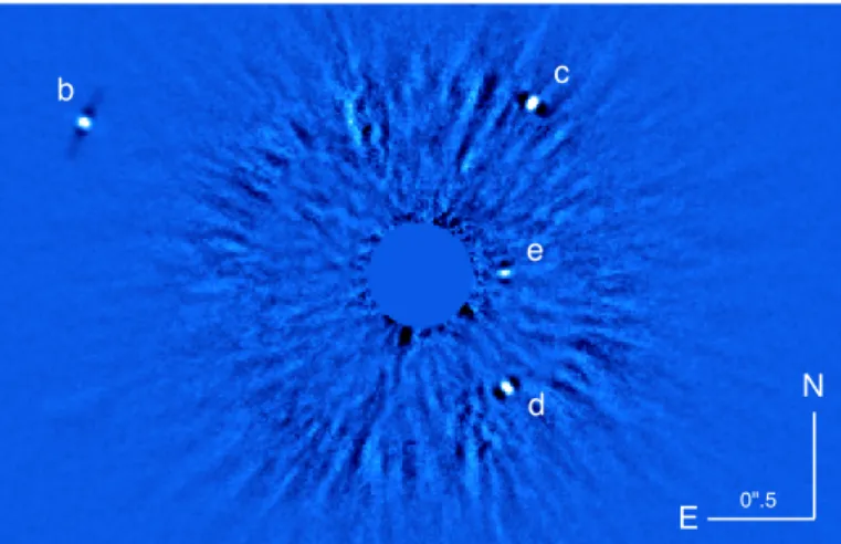
1 https://github.com/vortex-exoplanet/VIP 30 -23 -16 -9.3 -2.5 4.4 11 18 25 32 3 0".5 E N e d c b
Fig. 2. Illustration of a full-frame PCA ADI post-processed SPHERE/IRDIS image of HR8799 acquired with broadband H filter (left part) during the night of December 4, 2014. The central part was masked with a disk of radius 20 pixels.
algorithm implemented in VIP is based on the approach pre-sented inAmara & Quanz(2012), which can be summarized as follows:
– construct a set of orthogonal reference images, the so-called principal components (PCs), using singular value decompo-sition (SVD, see e.g.Press et al. 2007) of the data cube; – project all the frames of the cube onto a truncated set of nPC
(<nframe) PCs, where nframe represents the total number of
frames in a data cube;
– reconstruct the data cube using a linear combination of PCs, and subtract the result from the original data cube to obtain a cube of residual frames;
– rotate and collapse this cube of residuals to obtain the final image.
To optimize the determination of the astrometry, the S/N for each planet must be maximized. The S/N calculation implemented into VIP is based on a Student t-test (Student 1908) and fol-lows the recommendation ofMawet et al.(2014) on small sam-ple statistics (see Gomez Gonzalez et al. 2016b, for more de-tails). The S/N of the planets in the final, post-processed image depends mainly on the number of PCs used when building the re-constructed cube. A small number of PCs leads to an incomplete representation of the speckle noise, while a large number of PCs tends to capture the signal of the planet in the reconstructed cube, which leads to a lower algorithmic throughput for the planetary signal after subtraction. An optimum number of PCs can gener-ally be found to maximize the planet S/N (Meshkat et al. 2014). For each data cube, we thus performed a grid search on the num-ber of PCs to maximize the mean S/N in a region of one reso-lution element in diameter around each companion. The optimal nPC for each data cube is reported in Table1. Let us note that
the PCA implemented in VIP comes with several SVD libraries, such as the efficient randomized SVD (Halko et al. 2011) and the well-known LAPACK (see e.g.Anderson et al. 1990). We re-fer to Gomez Gonzalez et al. (2016a) for a complete discussion of all the SVD libraries available in VIP.
Figure 2illustrates a VIP post-processed image using full-frame PCA, where all the pixels of each full-frame are used at once to construct the reference images through SVD. The close region surrounding the host star is most affected by residual speckle noise and was masked with a disk of radius 20 pixels to better reveal the planets in Fig.2. Throughout the present analysis, we
Table 1. Final HR8799bcde astrometric measurements with respect to the host star for nights of December 4–6, and 8, 2014.
Date and side nPC ∆RA [00] ∆Dec [00] ∆r [00] ∆θ [◦] σstat,r[00] σstat,θ[◦] σspec,r[00] σspec,θ[◦]
HR8799b 2014-12-04 L 3 1.5754 0.7019 1.7247 65.985 0.0003 0.007 0.0002 0.007 2014-12-04 R 2 1.5750 0.7015 1.7242 65.994 0.0003 0.008 0.0002 0.007 2014-12-05 L 7 1.5761 0.7026 1.7256 65.975 0.0003 0.009 0.0002 0.009 2014-12-05 R 6 1.5760 0.7024 1.7254 65.977 0.0003 0.008 0.0002 0.008 2014-12-06 L 6 1.5730 0.7008 1.7221 65.985 0.0004 0.013 0.0002 0.009 2014-12-06 R 6 1.5739 0.7000 1.7225 66.023 0.0004 0.013 0.0002 0.009 2014-12-08 L 4 1.5743 0.7016 1.7236 65.980 0.0003 0.013 0.0003 0.011 2014-12-08 R 4 1.5736 0.7021 1.7231 65.956 0.0003 0.008 0.0003 0.010 HR8799c 2014-12-04 L 5 −0.5116 0.7971 0.9471 327.307 0.0002 0.014 0.0006 0.048 2014-12-04 R 6 −0.5127 0.7984 0.9488 327.293 0.0002 0.010 0.0006 0.044 2014-12-05 L 13 −0.5089 0.7992 0.9475 327.512 0.0003 0.012 0.0008 0.059 2014-12-05 R 14 −0.5103 0.8003 0.9492 327.479 0.0004 0.015 0.0008 0.053 2014-12-06 L 15 −0.5113 0.7979 0.9477 327.351 0.0005 0.020 0.0006 0.047 2014-12-06 R 18 −0.5118 0.7986 0.9485 327.342 0.0005 0.013 0.0007 0.052 2014-12-08 L 20 −0.5104 0.7987 0.9479 327.421 0.0004 0.026 0.0010 0.077 2014-12-08 R 7 −0.5128 0.7986 0.9491 327.291 0.0003 0.016 0.0012 0.088 HR8799d 2014-12-04 L 5 −0.3990 −0.5250 0.6594 217.233 0.0012 0.024 0.0012 0.093 2014-12-04 R 5 −0.3994 −0.5244 0.6592 217.292 0.0004 0.027 0.0011 0.092 2014-12-05 L 21 −0.4008 −0.5233 0.6592 217.448 0.0006 0.035 0.0013 0.085 2014-12-05 R 21 −0.3999 −0.5221 0.6576 217.454 0.0005 0.039 0.0013 0.075 2014-12-06 L 21 −0.4008 −0.5233 0.6592 217.446 0.0005 0.022 0.0010 0.077 2014-12-06 R 20 −0.3999 −0.5230 0.6584 217.397 0.0005 0.017 0.0010 0.080 2014-12-08 L 18 −0.3982 −0.5208 0.6556 217.405 0.0004 0.030 0.0029 0.136 2014-12-08 R 46 −0.4007 −0.5208 0.6571 217.575 0.0005 0.029 0.0027 0.123 HR8799e 2014-12-04 L 9 −0.3859 0.0117 0.3861 271.735 0.0010 0.103 0.0022 0.202 2014-12-04 R 16 −0.3852 0.0099 0.3854 271.468 0.0013 0.077 0.0039 0.292 2014-12-05 L 10 −0.3829 0.0121 0.3831 271.803 0.0006 0.044 0.0029 0.196 2014-12-05 R 12 −0.3841 0.0125 0.3843 271.859 0.0005 0.055 0.0024 0.167 2014-12-06 L 8 −0.3858 0.0097 0.3859 271.436 0.0006 0.034 0.0022 0.182 2014-12-06 R 23 −0.3865 0.0113 0.3867 271.668 0.0006 0.048 0.0019 0.159 2014-12-08 L 15 −0.3843 0.0139 0.3846 271.072 0.0016 0.186 0.0049 0.357 2014-12-08 R 11 −0.3862 0.0159 0.3865 272.360 0.0008 0.145 0.0082 0.534
Notes. The astrometric measurements are derived from SPHERE/IRDIS broadband H measurements (left and right parts), in terms of RA/Dec (Cols. 3–4) and in polar coordinates (Cols. 5–6). In addition, we list the derived optimal number of principal component nPC(Col. 2), as well as
the statistical error bars (Cols. 7–8) and the speckle noise error bars (Cols. 9–10), both in polar coordinates.
also performed annulus-wise PCA, which consists of performing PCA only for a thin annulus passing through a companion, with a typical width of a few resolution elements. Although full-frame PCA and annulus-wise PCA may lead to slightly different re-sults, this choice does not significantly affect the final astrome-try, which is dominated by other sources of error (see Sect.3). Furthermore, annulus-wise PCA is significantly faster when per-formed on a single annulus, which is useful when dealing with large data cubes and/or when PCA is performed a large number of times (see Sect.3.2).
3. Robust astrometry
The astrometric position of the HR8799bcde planets based on the December 2014 SPHERE/IRDIS data set has already been determined by Zurlo et al. (2016) and Apai et al. (2016). The Zurlo et al.(2016) final astrometry was obtained from the com-bination of four independent image-processing pipelines, by the quadratic sum of the error bar from each data reduction pipeline
plus the standard deviation associated to the individual positions. Apai et al.(2016) used their implementation of the KLIP algo-rithm to derive the planets positions by injecting artificial plan-ets with negative count rates, and used a manual inspection of the image quality and of the subtraction residuals to estimate the error bars. Here, we propose to go beyond these approaches and to study in detail the various contributions to the astrometric er-ror budget, in an attempt to derive more reliable erer-ror bars. Our study is also meant to explore the ultimate astrometric accuracy of a state-of-the-art instrument such as SPHERE, and to iden-tify possible ways to improve the astrometric accuracy in future studies.
What we call robust astrometry consists of performing a proper evaluation of the statistical errors and systematic biases affecting the final astrometric estimation. The whole procedure consists of four steps: (i) the description and estimation of the instrumental calibration errors; (ii) the determination of the plan-ets position with respect to the star and the related statistical er-ror through Bayesian inference with MCMC sampling; (iii) the
determination of the systematic error due to residual speckles, and (iv) the calculation of the error on the star position. Through-out the remainder of this section, we provide details for each step of the process.
3.1. Instrumental calibration and related errors
To derive accurate astrometric measurements from IRDIS images, various astrometric calibrations must be performed, namely the determination of the plate scale, the orientation of the north, and the optical distortion. Firstly, the plate scale, given in arcsecs per pixel, depends on the characteristics of all the op-tical elements composing the instrument. It allows conversion of positions given in pixels into arcsecs. Secondly, when observing in pupil-stabilized mode, the vertical axis of the detector does not necessarily point towards north. Two contributions need to be taken into account: (i) the pupil offset, which accounts for the zero point position of the derotator and is assumed to be con-stant between runs; and (ii) the so-called true north, which ac-counts for a variation in the detector orientation with respect to the sky due to thermal or mechanical stresses, and which must be estimated during each observing run. Thirdly, the distortion in SPHERE/IRDIS is mainly dominated by an anamorphic magni-fication between the horizontal and vertical axes of the detector. This effect is due to the presence of toric mirrors in the common path of the instrument (see e.g.,Zurlo et al. 2016).
Details of the observations used to derive those astromet-ric calibrations for IRDIS are described in Zurlo et al.(2016). We refer to that paper for the details, but we still provide the reader with the practical information used in this study. The as-trometric calibrations were obtained from IRDIS observations of the globular cluster 47 Tuc acquired on December 15, 2014, with the same instrument setup and filter, and were compared to the Hubble Space Telescope data of the same field, precessed to the same epoch and corrected for the differential proper mo-tions of the individual stars. The values derived byZurlo et al. (2016) for the plate scale and true north based on this data set have recently been revised by the SPHERE consortium, using their improved knowledge of the instrument. This revised esti-mation, described in Maire et al.(2016), leads to a plate scale of 12.251 ± 0.009 mas/pixels and a true north orientation of −1◦.709 ± 0◦.051. These values are valid for both the left and
right parts of the IRDIS detector. The pupil offset, based on commissioning and guaranteed-time data obtained on several as-trometric fields, is equal to 135◦.99 ± 0◦.11. Finally, the IRDIS
distortion measured on sky is dominated by an anamorphism of 0.60% ± 0.02% between the horizontal and vertical direc-tions (Maire et al. 2016). Although the SPHERE calibration plan includes the daily measurement of distortion maps based on pin-hole grids, we found that the quality of the astrometric estima-tions is not improved by using these maps. Prior to any post-processing, we thus simply rescaled each frame of each cube by a factor 1.006 along the y axis. To take into account the un-certainty on this correction, an additional error of 0.02% on the plate scale will be considered in the following analysis.
3.2. Planet position and statistical error
The next step in the robust astrometry process consists of de-termining, for each data cube, the position of the planets with respect to the host star and estimating the statistical error re-lated purely to the photon noise of the underlying thermal background and speckles through Bayesian inference based on
29 -22 -16 -8.7 -2 4.8 12 18 25 32 3
0".3
E
N
29 -22 -16 -8.7 -2 4.8 12 18 25 32 3
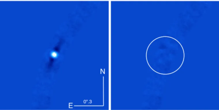
Fig. 3.Illustration of the annulus-wise PCA post-processing and merit function evaluation used in the negative fake companion technique. Left: no NEGFC was injected before annulus-wise PCA processing. Right: a NEGFC was injected at the position and flux minimizing the merit function. The white circle illustrates the fixed circular aperture from which the pixel values Ijhave been extracted to evaluate the merit
function. The same color-scale was used for both images.
MCMC simulations. This step does not describe the effect of the speckles themselves on the measured planet position, which will be discussed separately in Sect.3.3. Our astrometric mea-surements are based on the negative fake companion technique (NEGFC, see e.g. Marois et al. 2010a; Lagrange et al. 2010), which consists of injecting a negative PSF template into the data cube with the aim of canceling out the companion (as well as possible) in the final post-processed image based on a well-chosen merit function. The NEGFC technique is an iterative pro-cess, for which a step can be described as follows. For the chosen position/flux combination, a negative fake companion is injected into each frame of the data cube, and annular-wise PCA-ADI processing is performed on a single annulus passing through the considered companion. The intensities Ij of N pixels are then
extracted within a circular region with a radius equal to a few resolution elements, centered on a first guess position defined at the start of the iterative process (which means that the position of the circular aperture is fixed and does not change during the process). Assuming that the noise affecting the jth pixel value is given by σj = pIj(pure photon noise), we define the merit
function as follows: χ2∝ N X j=1 |Ij|. (1)
The position/flux of the NEGFC is then optimized to minimize the merit function in a three-step approach, as described in the following paragraphs. The resulting post-processed images, be-fore and after injection of a NEGFC, are represented in Fig.3. Because no off-axis PSF was acquired in December 2014 with the same observing setup as for the HR8799 observations, the adopted PSF template corresponds to unsaturated off-axis im-ages of β Pictoris obtained with SPHERE/IRDIS during science verification on January 30, 2015 (PI: A.-M. Lagrange) with the same observing mode as for HR8799 (same coronagraph, same broadband H filter, and similar seeing ∼100). The influence of this choice is discussed at the end of Sect.3.2, together with a discus-sion of the effect of PSF chromatic dispersion on the measured planet position.
First guess estimation. With the optimal number of PCs in hand (see Table1), we derive a first guess of the position of each companion in each PCA-ADI post-processed image by simply
identifying the highest pixel value in the close vicinity of the companion. We then derive a first guess of the flux of the com-panion by injecting a NEGFC at that position and by evaluating the merit function for a grid of possible fluxes. Only the flux is optimized during this stage, while the companion position is fixed to our first guess.
Nelder-Mead optimization. Although the first guess estimation results in a rough determination of the position/flux, and would constitute a valid initial set of parameters to start an MCMC-based Bayesian inference process (as presented in the next para-graph), it may turn out to be very time consuming due to the large number of merit function evaluations required to reach conver-gence in the MCMC and properly sample the posterior distri-butions. Thus, we propose to refine the first guess of the posi-tion/flux of the companions for the purpose of initializing the MCMC sampling close to the highly probable solution. To this end, we use the first position/flux estimation as an initial guess for a Nelder-Mead simplex-based optimization (Nelder & Mead 1965) implemented into the SciPy Python library2. The adopted merit function is defined in Eq. (1), and the position (r, θ) of the NEGFC is now allowed to vary during the fit in addition to its flux. As expected, this leads to a significant improvement of the position/flux determination. The right panel of Fig.3 illus-trates the result of an annulus-wise PCA-ADI post-processing performed on a single annulus passing through HR8799b, after injecting a NEGFC characterized by a position and flux mini-mizing the merit function.
The PCA-ADI algorithm that we first used in VIP relied on a randomized SVD library, which approximates the SVD of the data cube by using random projections and thereby pro-vides increased computational efficiency (for details see Gomez Gonzalez et al. 2016a). Although this randomized approach is very efficient, the random process induces random variations in the merit function that can be significant compared to the vari-ations of the merit function between two steps, especially when approaching the minimum. This can prevent the optimization process from reaching the true minimum of the merit function, or even from converging. Therefore, we decided to use the more classical, yet slower, deterministic SVD approach proposed in the LAPACK library for our PCA-ADI processing in the simplex optimization, as well as for the rest of this study. This choice is all the more important when the companion is located in a region dominated by residual speckle noise.
MCMC and final positions. Because the merit function used in the Nelder-Mead optimization is not strictly convex, it is not guaranteed that the optimization will converge at the exact posi-tion of the planet, as it could potentially get stuck in a local min-imum. Although this behaviour was generally not observed (as shown inMorzinski et al. 2015), we decided to use the NEGFC technique coupled with an MCMC approach to obtain the final flux and position of the HR8799 planets, expressed in polar coor-dinates, with respect to the host star. Let us recall briefly that the MCMC approach aims to sample the posterior probability den-sity function (PDF), that is the probability of the position/flux parameters given the data cube and the prior knowledge (see e.g. Hogg et al. 2010). The VIP module dedicated to the NEGFC technique embeds the emcee package (Foreman-Mackey et al. 2013), which implements an affine-invariant ensemble sampler for MCMC proposed by Goodman & Weare (2010). Such an
2 http://www.scipy.org
Fig. 4.Illustration of a typical corner plot obtained from the MCMC simulations using the NEGFC technique. The target companion is HR8799b observed during the night of December 6, 2014. The radial distance r (in pixels) and azimuth θ (in degrees) are detector coordi-nates with respect to the host star. The diagonal panels illustrate the posterior PDFs while those off-axis illustrate the correlation between them.
ensemble is composed of walkers, which can be considered as Metropolis-Hastings chains. The main difference between walk-ers and Metropolis-Hastings chains lies in the fact that the pro-posal distribution for a given walker depends, at a given step, on the position of all other walkers in the ensemble. Con-versely, the proposal distributions involved in the Metropolis-Hastings algorithm are independent. Besides being more e ffi-cient in terms of the number of calls to the cost function, one major advantage of emcee is that it relies on only two cali-bration parameters, in comparison to the ∼N2 parameters re-quired for a Metropolis-Hastings algorithm in an N-dimensional parameter space to properly sample the PDF and speed up the process (for more details, seeForeman-Mackey et al. 2013; Goodman & Weare 2010, and references therein).
For each data cube and each companion, we carried out MCMC simulations to sample posterior PDFs related to the planet polar coordinates (r, θ) with respect to the host star and the planet flux f . For each MCMC simulation, we used 200 walk-ers firstly initialized in a small ball around the solution obtained from the Nelder-Mead optimization. The chain was sufficiently close to convergence to allow Bayesian inference after, typi-cally, 200 steps. More details concerning convergence statistical tests are given in Sect.4.1, where we describe the PyAstrOFit Python package. In Fig. 4, the so-called corner plot illustrates the posterior PDFs and the correlation between the parame-ters (r, θ, f ) for HR8799b observed during the night of Decem-ber 6, 2014. Similar results were obtained for other planets and observing nights. Although a flux estimation for each planet is obtained, we focus our analysis on only the astrometry in this paper.
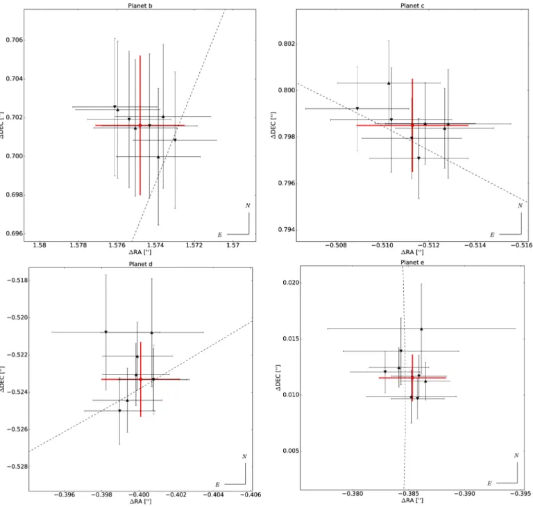
Taking into account the plate scale, the true north and pupil offset orientation (see Sect. 3.1), we have projected the HR8799bcde highly probable sets of polar coordinates onto the
Fig. 5.Astrometry for HR8799bcde observed during the nights of December 4–6, and 8, 2014. The positions obtained from the left (resp. right) data cubes are represented with downward (resp. upward) black triangles. The error bars on the individual data points take into account all the contributions discussed in Sects.3.1–3.4. The red dots correspond to the final astrometric measurements for each planet, together with the final error bar discussed in Sect.3.5. The dashed lines represent the best orbital solutions for each planet in terms of reduced χ2reported in Table5.
north and east directions. As a result, the eight HR8799bcde final positions for the four nights (left and right parts) are reported in Table 1 and displayed in Fig. 5. These positions will be used in Sect. 3.5 to deduce the final HR8799 astrometry for epoch 2014.93. In addition to obtaining the highly probable po-sition/flux for a given companion, the MCMC simulations give a robust estimation of the statistical error on the astrometry (i.e., related purely to photon noise). This error, reported in Cols. 7 and 8 of Table1, generally constitutes a minor contribution to the error budget, as discussed in the following sections.
Influence of the template PSF. Since a non-saturated, o ff-axis PSF was not obtained in the same observing mode during
the nights where HR8799 was observed, we chose, as a PSF template for our NEGFC analysis, the closest off-axis PSF in time obtained with the same observing mode under similar weather conditions, which turned out to be an off-axis PSF of beta Pictoris obtained on January 30, 2015. The fact that both the instrument and the atmospheric conditions may have changed within the interval leads to a possible bias in our measurement of the planets’ position, which could vary from night to night. To evaluate this bias, we took a series of twelve off-axis PSFs served in the same mode under good atmospheric conditions, ob-tained in 2015 in the context of the SHARDDS survey (J. Milli, priv. comm.). For each planet and each observing night in our HR8799 data set, we successively used the twelve off-axis PSFs
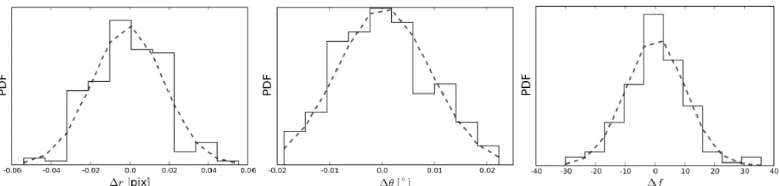
Fig. 6.Speckle noise estimation for HR8799b observed on December 6, 2014. The histograms illustrate the offsets between the true position/flux of a fake companion and its position/flux obtained from the NEGFC technique. The dashed lines correspond to the 1D Gaussian fit from which we determine the speckle noise.
as templates for the NEGFC technique, and derived the planets’ astrometry using the method described above. The dispersion of the astrometric measurements gives us an estimation of the bias that can be introduced by using a non-contemporaneous PSF. The observed dispersion does not depend significantly on the planet nor on the observing night, and has an overall standard deviation of 0.6 mas. This error bar will be added quadratically to the other error sources in Sect.3.5.
Influence of residual dispersion. Another source of imperfec-tion in the recovery of the planets astrometry for broadband ob-servations is the residual atmospheric dispersion after correction by the atmospheric dispersion correctors (ADC) included in the SPHERE optical path. While the small angular separation be-tween the star and planets ensures the residual dispersion to be almost perfectly equal for all of them, their different spectra can result in a chromatic offset between their measured positions. The residual dispersion after correction by the SPHERE ADC has been shown to be smaller than 1.2 mas rms for zenith angles as large as the maximum of 54◦encountered in the present data set (Hibon et al. 2016). Taking into account the H-band spec-trum of the star and of the four planets (Bonnefoy et al. 2016), we estimate that the maximum astrometric offset between the star and planets due to residual dispersion cannot be larger than 0.25 mas in the worst case where residual dispersion shows a linear trend across the H band. This contribution is negligible in our final astrometric error budget.
3.3. Systematic error due to residual speckles
Performing PCA-ADI removes a large fraction of the quasi-static speckle noise and significantly improves the S/N of the companions. Although highly effective, this process is not per-fect and some level of residual speckle noise remains in the post-processed images. Such noise has a major impact on pho-tometric and astrometric measurements (Guyon et al. 2012), and needs to be taken into account in the error budget. Since speckle noise is known to have a radial dependence, we propose to esti-mate its impact by injecting fake companions into the data cube at the radial distance of the real planets but for a wide range of angular positions, and by testing the ability of the Nelder-Mead optimization to find their position and flux through the NEGFC technique. The first step in this process is to create an “empty” data cube by injecting four NEGFCs characterized by the highly probable positions/fluxes derived from the previ-ous MCMC simulations. In the empty cube, we inject a fake
companion characterized by a flux ftrueand a radial distance rtrue,
both corresponding to the highly probable solution, but at an arbitrarily chosen angular coordinate θtrue,i. Using the NEGFC
technique coupled with the Nelder-Mead optimization, we deter-mine the position/flux (ri, θi, fi) of the fake companion. We then
compute the offsets ∆ri= rtrue−ri,∆θi= θtrue,i−θi,∆ fi= ftrue− fi
between the known position/flux characterizing the fake com-panion and the solution obtained from the optimization process. The same process is repeated for a series of 360 azimuths equally spaced between 0◦ and 360◦. These 360 realizations are used
to build three normalized histograms, for ∆r, ∆θ and ∆ f , re-spectively. The histograms for∆r and ∆θ are then fitted with a Gaussian function, and the standard deviations σspec,rand σspec,θ
of the Gaussian functions are used as an estimation of the speckle noise affecting the radial and azimuthal coordinates. A similar approach was already used byMaire et al.(2015), for example. We illustrate in Fig. 6 the three histograms for HR8799b ob-served on December 6, 2014. The results obtained for all plan-ets and data cubes are reported in Cols. 9 and 10 in Table1. It appears clear that the error induced by speckle noise increases for decreasing angular separations of the companion with re-spect to the host star. Indeed, the brightness of the residual speckles increases closer to the star. We also note that speckle noise is consistently larger than statistical noise, except for HR8799b.
Another possible way to evaluate speckle noise is to mea-sure the influence of the number of PCs used in the PCA post-processing on the position/flux determination, as proposed by Pueyo et al. (2015), for example. Indeed, the residual speckle pattern changes as a function of the number of PCs. To verify the consistency of this method with the one proposed above, we de-termined the position/flux of each companion in each data cube using the NEGFC technique with the Nelder-Mead optimization using a number of PCs ranging from 5 to 90 (for a number of PCs > 90, the companion self-subtraction becomes too signifi-cant to get a high S/N). We then constructed three normalized histograms, for r, θ and f . As expected, the standard deviations of these histograms are similar to those deduced above.
Finally, we note that the residual speckle noise estimated here is in good agreement with the semi-empirical estimation of the astrometric accuracy based on the planet S/N proposed in the case of pure photon noise byGuyon et al.(2012, Eq. (A1)), pro-vided that we extrapolate this relation to the speckle-dominated regime in the following way, as already proposed byMawet et al. (2015): σ1D[λ/D]= 1/(πS/N). Using such a semi-empirical
for-mula therefore seems to be a possible method to acquire a rapid estimation of the astrometric error bar related to speckle noise,
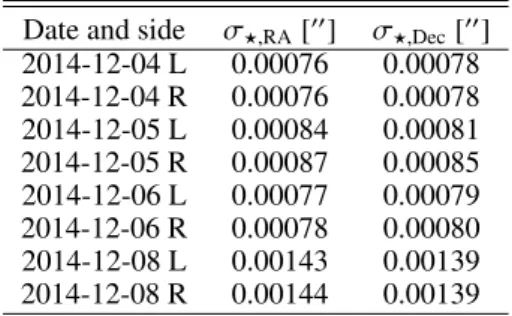
Table 2. Estimation of the stellar jitter in the eight data cubes.
Date and side σ?,RA[00] σ ?,Dec[00] 2014-12-04 L 0.00076 0.00078 2014-12-04 R 0.00076 0.00078 2014-12-05 L 0.00084 0.00081 2014-12-05 R 0.00087 0.00085 2014-12-06 L 0.00077 0.00079 2014-12-06 R 0.00078 0.00080 2014-12-08 L 0.00143 0.00139 2014-12-08 R 0.00144 0.00139
although we recommend going through the analysis presented in this section to obtain a robust estimation.
3.4. Error on the star position
Inside SPHERE, a dedicated differential tip-tilt sensor is used to obtain an image of the PSF immediately upstream of the coro-nagraph, and is used as an input for closed-loop control of the star position with respect to the coronagraph, thereby ensuring a stable star centering (Fusco et al. 2006; Baudoz et al. 2010). Based on laboratory measurements, the expected accuracy of the star centering is considered to be approximately 0.5 mas on sky (Baudoz et al. 2010). As mentioned in Sect.2.2, no individual frame centering was applied to the data cubes in our analysis, but rather a global centering of all frames in each individual cube using the same x, y offsets.
Here, we independently estimate the uncertainty on the mean star position for each data cube. The evaluation of this uncer-tainty is based on the histogram of the x and y offsets mea-sured for all individual frames by the centroid plus intersection method described in Sect. 2.2. The mean position of the star in a given data cube can be obtained by a Gaussian fit of the two histograms, as illustrated in Fig.1. Based on this figure, in the following discussion we assume that the histograms follow a Gaussian distribution, so that the accuracy on the determina-tion of the mean stellar posidetermina-tion in a given cube is given by the standard deviation of the best-fit Gaussian divided by the square root of the number of realizations. The standard deviations of the best-fit Gaussians are given in Table2in terms of right ascension (RA) and declination (Dec), by projecting the (σ?,x, σ?,y)-error ellipses expressed in detector coordinates onto the north and east directions. We note that the derived stellar jitter estimation is slightly larger than predicted inBaudoz et al.(2010), with val-ues varying from 0.76 mas to 1.44 mas depending on the night (i.e., around 0.1 pixel in detector coordinates). Based on these values, and taking into account the ∼200 frames present in each data cube, the error bar on the mean stellar position in any given cube amounts to less than 0.1 mas, and is therefore completely negligible in our final noise budget.
However, this contribution represents only the purely statisti-cal error on the determination of the star position. We also need to take into account possible systematic biases on the determi-nation of the star position based on the satellite spots. To this end, we obtained a data set on a relatively bright star, using the waffle mode of the DM, but without coronagraph. The star was mildly saturated at its center to increase the S/N on the satellite spots. We determined the center of the star based on a truncated Moffat profile to reject the saturated part of the PSF, and com-pared this estimation with the prediction based on the satellite spots. We verified that the two estimations match with an accu-racy better than 0.1 pixels, which represents our best estimation
of an upper limit on a possible bias. This also confirms that the method proposed in Sect.2.2, to determine the stellar position from the satellite spots, does not lead to major astrometric bias, even in the presence of residual atmospheric dispersion. Here, we conservatively assume that a bias of 0.1 pixels (1.2 mas) af-fects our determination of the mean star position in all cubes.
3.5. Final astrometry
Particular care must be taken when combining the results and error bars of several astrometric measurements, especially in the presence of correlated errors. How the various error bars add up requires specific discussion. Firstly, we note that our experi-mental determination of the error bar related to residual speckles inherently takes into account the contribution of photon noise. Indeed, the empirical intensity of the speckles includes the con-tribution of the photon noise associated to all sources of signal at any given location (stellar residuals, planet, sky emission and thermal background). This is supported by the fact that the er-ror bar associated to speckle noise generally dominates the erer-ror bar associated to photon noise. Only in the case of planet b are they of the same order of magnitude, which reflects the fact that residual speckles are very faint compared to residual background noise at that angular distance from the star.
Secondly, we make the conservative assumption that the er-rors related to speckle noise are fully correlated, not only be-tween the left and right data cubes obtained on the same night, but also between all nights. The assumption of full correlation between the left and right data cubes is justified by the fact that the signals recorded by the two parts of the detector are almost identical (to within photon noise and some minor differential aberrations that amount to a few nm rms at most), and is backed up by the fact that the estimated error bars are almost identical for the left and right sides for most of the nights and planets (see Table1). The assumption that speckle noise is fully corre-lated from night to night is more debatable. It is indeed expected that speckle noise will be partly correlated between successive nights, because residual speckles are often associated to non-common path aberrations in the instrument that can vary on very long timescales. To remain on the conservative side, we will as-sume a full correlation of speckle noise in all data sets. The er-ror bar on the final astrometry regarding speckle noise should then be computed as the median of all speckle noise-related error bars. We note however that the estimations of the speckle noise-related error bars significantly vary from one night to another (see Table1), which suggests that this noise is at least partly un-correlated, and that our final error bars will be pessimistic.
Thirdly, we proposed in the previous section that the final error bar related to the determination of the star position is dom-inated by a systematic bias that can amount to 1.2 mas, and that the variability of the PSF shape can induce a bias of up to 0.6 mas. These biases will be added quadratically to our final as-trometric error bar for all planets. The same applies to instrumen-tal calibration errors, which are supposed to affect all data cubes in the exact same way. Indeed, appropriate observations of as-trometric fields were not performed on each of the five HR8799 observing nights. We therefore had to rely on an astrometric cal-ibration carried out by the SPHERE consortium one week later (see Sect.3.1), which was used as a reference for all five nights. Although we could not check the stability of the calibration over several nights, we note that the latest IRDIS astrometric calibra-tions by the SPHERE consortium show that the time variacalibra-tions of plate scale and true north are mostly within their estimated error bars, based on two years of astrometric field observations,
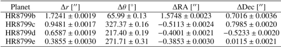
Table 3. The final HR8799bcde astrometric measurements with respect to the star for epoch 2014.93.
Planet ∆r [00] ∆θ [◦] ∆RA [00] ∆Dec [00]
HR8799b 1.7241 ± 0.0019 65.99 ± 0.13 1.5748 ± 0.0023 0.7016 ± 0.0036 HR8799c 0.9481 ± 0.0017 327.37 ± 0.16 −0.5113 ± 0.0024 0.7985 ± 0.0020 HR8799d 0.6587 ± 0.0019 217.40 ± 0.19 −0.4001 ± 0.0021 −0.5233 ± 0.0020 HR8799e 0.3855 ± 0.0030 271.71 ± 0.31 −0.3853 ± 0.0030 0.0115 ± 0.0021
while the pupil offset and anamorphic factor are mostly constant (Maire et al. 2016). This suggests that our final estimation of the astrometric error bar should not include any unaccounted bias related to the variability of the IRDIS astrometric calibration. That being said, we still recommend that, in future observing programs dedicated to precise astrometric measurements, obser-vations of standard astrometric fields be obtained during each individual night to ensure a high astrometric robustness.
Based on these assumptions, the computation of the final astrometry and related error bars proceeds as follows for each planet:
– define the final astrometry of the four planets as the weighted mean of the eight individual positions (left and right parts of the detector for the four nights), using the inverse of the variance of speckle noise as a weight;
– estimate the final error bar related to speckle noise as the median of the individual error bars on the eight astrometric measurements;
– add quadratically; the contribution of speckle noise, the up-per limit on the stellar centering bias, and the contribution of instrumental calibration errors to obtain the final astrometric error bars.
All these calculations are performed in polar coordinates, re-flecting the fact that error bars generally have different behaviors along the radial and azimuthal directions. The last step is based on the following formulae:
σ2 tot,r= PLSC 2 (σ2r,spec+ σ2r,?+ σ2r,PSF+ σ2r,AFr2)+ σ2PLSCr 2, (2) σ2 tot,θ = σ 2 θ,spec+ σ2θ,?+ σ2θ,PSF+ σ2θ,AF+ σ2PO+ σ 2 TN, (3)
where r is the radial distance in pixels, σr,specand σθ,specthe
fi-nal radial (pixels) and azimuthal (degrees) error bars related to speckle noise, σr,? and σθ,? the radial (pixels) and azimuthal (degrees) stellar centering biases, σr,PSF and σθ,PSF the radial
(pixels) and azimuthal (degrees) error bars related to the imper-fection of the PSF template in the NEGFC analysis, σr,AFand
σθ,AF the radial and azimuthal errors on the anamorphic factor expressed as percentages, and where PLSC refers to the plate scale in00/pixel, PO to the pupil offset and TN to the true north, both in degrees. The final astrometries and related error bars are given for the four planets in Table3and are illustrated in Fig.5. Table3includes a projection of the error bars onto the RA and Dec directions, to comply with the usage. However, we suggest that expressing the error bars in polar coordinates is more appro-priate, because polar coordinates usually correspond to the major and minor axes of the error ellipse. Another, even more appro-priate way to proceed would be to specify the error ellipse by its three parameters (two axes and position angle). In the present case, the error bars are sufficiently symmetric to proceed with RA/Dec error bars, even though we note that the HR8799b er-ror bars are significantly asymmetric, the angular erer-ror bar being twice as large as the radial one. This is mostly due to the large un-certainty on the pupil offset (0◦.11, see Sect.3.1), which severely
affects planets located far from the star.
Table 4. Comparison between the final error bars (σtot) listed in Table3
and the standard deviation of the eight positions per planet displayed in Fig.5(see also Table1).
Planet σtot,∆RA σ(∆RA) σtot,∆Dec σ(∆Dec)
[mas] [mas] [mas] [mas]
HR8799b 2.3 1.1 3.6 0.8
HR8799c 2.4 1.2 2.0 0.9
HR8799d 2.1 0.9 2.0 1.4
HR8799e 3.0 1.2 2.1 1.9
To verify the consistency of our error bars, we compared the statistical distribution of the eight individual data points ob-tained for each planet to the individual error bars on the eight data points. Table4shows that the final error bars are generally approximately twice larger than the dispersion of the individual data points. This is related to the fact that the major error sources (speckle noise, stellar position bias, and instrumental calibration) are supposed to be fully correlated between individual measure-ments, so that the final error bar has a similar size as the indi-vidual ones. This suggests that an improvement by up to a fac-tor two in astrometric accuracy could be achieved by improving the astrometric calibration. That said, the individual error bars are in relatively good adequacy with the dispersion of the data points (see Fig.5), although we note a significant asymmetry in the distribution of the data points towards the NE-SW direction. This asymmetry appears relatively consistent between the four planets, and we therefore suggest that it comes from a time vari-ability in the bias on the stellar position measurement (the only error source that is naturally expressed in RA/Dec), which could be related to variations in the PSF shape and/or in the diffrac-tion pattern created by the DM on a night-to-night timescale. This variation remains within the expected amplitude of approx-imately 0.1 pixels for the star position bias.
For planet b, the main contribution to the error budget comes from the imperfect astrometric calibration and from the uncer-tainty on the star position, while speckle noise is negligible. This is consistent with the fact that HR8799b lies in a region that is not significantly affected by residual speckles (see Fig.2). For planet c, although speckle noise significantly increases, the noise budget remains dominated by the astrometric calibration and stellar position uncertainties. The dominance of stellar cen-tering noise in the astrometric error budget of these two planets is supported by the fact that the dispersion in the individual astro-metric measurements for planets b and c has a similar amplitude and shape (see Fig.5), as is expected for a global centering error. For the two inner-most planets (d and e), speckle noise progres-sively becomes the dominant contributor to the error budget, and once again this is consistent with Fig.5, where the dispersion of the astrometric data points increases significantly, especially for planet e. We finally note that our astrometric measurements are in general agreement with the astrometric measurements derived inZurlo et al.(2016) andApai et al.(2016) to within error bars, but that our error bars are two to three times smaller, thanks to a
careful evaluation of all systematic error sources. For the orbital architecture analysis presented in the next section, we will thus only use our data reduction for the IRDIS data set of December 2014.
4. Orbital fitting analysis
4.1. The PyAstrOFit Python package
To perform our analysis of the HR8799bcde orbital architecture, we adopted the Bayesian framework. With the aim of making our results reproducible as well as allowing anyone to straightfor-wardly perform similar analyses, we introduce the PyAstrOFit package3 implemented in Python 2.7, which is fully dedicated
to orbital fitting using the MCMC approach. The code is open source and has been used to carry out our analysis and to pro-duce all the figures presented in this section. PyAstrOFit is composed of several modules, but the core of the package re-lies on three main modules, referred to as Orbit, Sampler and Inference:
– The Orbit module is used to instantiate an orbit object, which includes the required data to model or represent any bound orbit. Unbound orbits are not considered because they would require the use of universal Keplerian variables and Stumpff functions (Beust et al. 2016).
– The Sampler module constitutes the core of the Markov chains construction. It embeds the emcee package (Foreman-Mackey et al. 2013), which implements the affine-invariant ensemble sampler for MCMC proposed by Goodman & Weare(2010).
– The Inference module is dedicated to Bayesian inference. Its main purpose is to represent both the posterior PDFs and the correlations between parameters from the Markov chain, to determine the confidence intervals, and to derive a set of allowable orbits or the best solution in terms of reduced χ2.
The PyAstrOFit sampler comes with several convergence di-agnostic tools. In practice, one can never be sure that a chain has actually converged, but there exists several tests to evaluate whether the chain appears to be close to convergence (or more precisely, far from non-convergence4):
– The acceptance rate (MacKay 2003), which corresponds to the fraction of accepted to proposed candidates, can be moni-tored: if the acceptance rate is too high, the chain is probably not mixing well, while a low acceptance rate indicates that too many proposed candidates are rejected (which is symp-tomatic of a walker stuck in a given position).
– The Gelman-Rubin ˆRstatistical test (Gelman & Rubin 1992; Ford 2006;Gelman et al. 2014) compares, for each parame-ter, the variance estimated from non-overlapping parts of the chain to the variance of their estimates of the mean. A large
ˆ
Rvalue may arise from slow chain mixing or multimodal-ity (Cowles & Carlin 1996). Conversely, a ˆRvalue close to 1 indicates that the Markov chain is close to convergence. – The lag ρkautocorrelationcorresponds to the correlation
be-tween every draw and its kth lag. A relatively high ρk=Kvalue
for a given K indicates a high degree of correlation between the draws, a slow mixing and a chain far from convergence. – The integrated autocorrelation time τ (see e.g.
Foreman-Mackey et al. 2013; Christen & Fox 2010; Goodman & Weare 2010), also called inefficiency factor,
3 https://github.com/vortex-exoplanet/PyAstrOFit 4 In the rest of the text, we will generally use “convergence” as an
abbreviation of “far from non-convergence”.
aims to give an estimate of the number of posterior PDF evaluations required to draw an independent sample. The smaller τ, the better.
Following Ford (2006) and Chauvin et al. (2012), the sam-pling can be done on three different state vectors noted x = (a, e, i, ω,Ω, tp), x0 = (log P, e, cos i, Ω + ω, Ω − ω, tp) where P
represents the orbital period, and u(x) defined at Eq. (A.1) in Chauvin et al.(2012). As suggested byFord(2006), adopting a uniform prior distribution for x0may help to improve the
conver-gence of the chain. Indeed, a uniform prior distribution for cos i in the interval [−1, 1] implies a prior distribution proportional to sin i in the interval [−90◦, 90◦] for the inclination. As a conse-quence, it implies that orbits characterized by i ' 0◦ (face-on)
are considered intrinsically less probable than those character-ized by i ' 90◦(edge-on).
Which statistical test one should adopt as a convergence criterion is a question with no trivial solution. Nonetheless, some recommendations can be found in the literature (see e.g. Cowles & Carlin 1996). For instance,Gelman et al.(2014) the-oretically demonstrated that the optimal Markov chain mixing to sample normally distributed posterior PDFs is characterized by an acceptance rate equal to ∼0.44 when adopting the Metropolis-Hastings algorithm. It is widely agreed that an acceptance rate between 0.2 and 0.5 constitutes an appropriate value to ensure a good Markov chain mixing. The criteria adopted in this anal-ysis are defined in the following section where we address the HR8799 orbit fitting, and are generally similar to those used by Pueyo et al.(2015) in their study of the HR8799 orbital param-eters. When all the statistical tests meet the criteria, we con-sider that the part of the chain satisfying them has converged. The Inference module can then be used to draw independent samples from the chain to construct the final posterior PDFs for each Keplerian parameter. The confidence intervals are defined in terms of highest density regions (HDR,Hyndman 1996), also referred to as highest posterior density intervals. For a given con-fidence level 1 − α (0 ≤ α ≤ 1), the idea is to take a horizontal line and shift it up until the area under the regions of the PDF located above this line represents a fraction 1 − α of the total area under the PDF. The projection to the x axis of this area de-fines the 100(1 − α)% HDR. To infer our confidence intervals, we chose to use the 68.3% HDRs. In the ideal case where the PDF f is unimodal, the HDR corresponds to the smallest of all intervals [a, b] that satisfy Pr(a ≤ x ≤ b)= 1 − α, which happens such that f (a)= f (b).
The Inference module also comes with various tools to dis-play the results, such as corner plots to illustrate the PDFs and their corresponding correlation, walk plots to illustrate the mix-ing of the chain, and the illustration of allowable orbits together with the data. More information about all the PyAstrOFit pos-sibilities and tutorials dedicated to each module can be found in the GitHub repository.
4.2. HR8799 orbital fitting with PyAstrOFit
Here, we revisit the MCMC-based Bayesian analysis described inPueyo et al.(2015) using more robust convergence criteria be-fore using our chains for inference, and using an extended data set by adding not only the SPHERE astrometric data presented in this work but also the latest astrometric measurements from the literature (see below). We update those results to what is described in this section. As a consequence, this analysis super-sedes that presented inPueyo et al.(2015).
For our orbital analysis, we assumed the distance of the sys-tem and the mass of the host star to be 39.4 pc (van Leeuwen 2007) and 1.51 M (Baines et al. 2012), respectively. The
possi-bility of inferring these parameters from the orbital fitting mod-ules has not been implemented into PyAstrOFit yet, but could be the subject of a future update. The astrometric positions used for the orbit fitting come from the works ofMarois et al.(2008), Lafrenière et al. (2009),Fukagawa et al.(2009),Metchev et al. (2009), Hinz et al. (2010), Currie et al. (2011, 2012, 2014), Bergfors et al. (2011), Galicher et al. (2011), Soummer et al. (2011), Esposito et al. (2013), Maire et al. (2015), Zurlo et al. (2016), and Konopacky et al. (2016) along with the positions derived in the present work. A compilation of all the astromet-ric measurements for HR8799bcde is provided in TableA.1. All these data are included in the PyAstrOFit source code, and can easily be queried by an interested user.
The presence of systematic errors, whose careful calibra-tion is described in Sect.3, turned out to be a significant nui-sance when trying to reconcile contemporaneous astrometric measurements from various instruments. For instance, the dif-ference in astrometry for HR8799b betweenCurrie et al.(2014) andPueyo et al. (2015) could be explained by an offset in the true north position between Palomar and Keck (this offset has a lesser impact for the planets at smaller separations). Given the relative paucity of data in the astrometric calibrator (based on a single astrometric binary) presented inPueyo et al.(2015), compared to the long history of high precision Keck astrome-try (see e.g., Yelda et al. 2010; Service et al. 2016), we chose to include only the Currie et al.(2014) points in our analysis. Another example would be the discrepancy for the position of HR8799d between these two papers, which can be easily traced back to the presence of a bright residual speckle near planet d in the Palomar/P1640 data. Because there is no CPU-efficient method to carry out the negative injection in IFS data without ADI,Pueyo et al.(2015) could not use the method described in Sect. 3.1, and only used a method similar to that presented in Sect. 3.3(at other azimuth angles, where there was no bright speckle). As a consequence the Pueyo et al. (2015) uncertain-ties on HR8799d are most likely under-reported, and we instead use the contemporaneous estimate ofCurrie et al.(2014). These two examples illustrate the complexity of precision astrometry in high contrast imaging and the importance of carrying out all the steps of robust astrometry as described in the present paper. Be-cause the HR8799 system has been observed by multiple instru-ments since 2012, and because we had access to the P1640 data, we could conduct these instrument to instrument sanity checks and choose the most robust published astrometry. Before 2012, the measurements are more sparse and we thus decided to in-clude all of them in the orbit fitting in the absence of further information.
The affine invariant sampler implemented in emcee comes with only two hyperparameters to be tuned: the number of walkers and an adjustable scale parameter a > 1, which has a direct impact on the acceptance rate of each walker (see Goodman & Weare 2010). All our simulations were performed with 1200 walkers. For a given Keplerian parameter, the set com-posed of the first element of each walker constitutes the ini-tial distribution, which depends on how we decide to iniini-tialize the walkers. The equilibrium distribution, which we expect to be close to the posterior distribution when the chain has con-verged, should not depend on this initial distribution (see e.g. Meyn & Tweedie 2009). As discussed inForeman-Mackey et al. (2013), starting the simulation with an initial distribution close to the expected posterior distribution speeds up the convergence.
This can be done by initializing the walkers in a small N-dimensional ball in the parameter space around a highly prob-able solution. However, such an approach not only requires a priori knowledge of the main posterior distribution peak, but can also jeopardize the chain convergence if the posterior dis-tribution is multi-modal. Various alternatives are proposed in Foreman-Mackey et al. (2013), and we have tested some of them. In particular, we can start the walkers uniformly over a given range in the parameter space. All our tests have led to iden-tical results for all the Keplerian elements of each planet.
We have started the chain construction with a minimum of 1000 steps per walker before beginning any convergence tests. During the MCMC run, the acceptance rate was monitored and the hyperparameter a (initially set to 2) was dynamically tuned in order to ensure an acceptance rate between 0.2 and 0.5 for at least 75% of the walkers. The walkers for which acceptance rate was outside [0.2, 0.5] were discarded and not used for Bayesian inference. We considered that a chain has converged when the Gelman-Rubin statistical test ˆR< 1.01 is satisfied three times in a row for all Keplerian parameters. The convergence was reached after typically 40 000 steps per walker, for a total computing time equal to three hours using a computer equipped with 28 process-ing units.
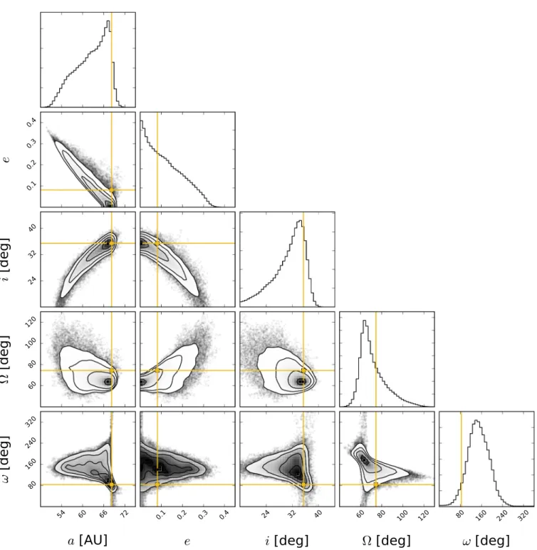
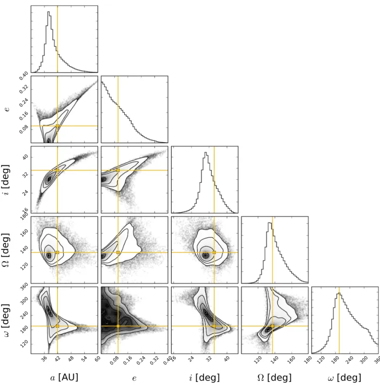
For each planet, the corner plots are depicted in Figs.7 to 10. They illustrate the resulting posterior PDFs and the corre-lation between the Keplerian parameters a, e, i,Ω and ω. The yellow lines represent the best solution in terms of reduced χ2. These solutions do not necessarily coincide with the peaks of the posterior PDFs. Following the procedure described in Sect.4.1, the confidence intervals were inferred from the posterior PDFs and are summarized in Table5 together with the best solution in terms of reduced χ2. In addition, Figs.B.1andB.2illustrate a set of 1000 allowable orbits characterized by χ2 < χ2
min+ 0.1
and for which all the Keplerian parameters are in the confidence intervals reported in Table5.
4.3. Discussion
One of the most striking results of our MCMC analysis concerns the eccentricity of planet d, which shows a clear peak around ed, peak ∼ 0.35, and rejects the circular orbit hypothesis outside
its 1σ confidence interval (although a significant set of solutions characterized by ed < 0.2 cannot be ruled out). Actually, all four
planets show possible signs of non-circular orbits at various lev-els, as the eccentricity posterior PDFs are generally rather broad, or in some cases (planets d and e) not monotonically decreasing. Another striking result concerns the orientation of the orbits. The inclination of all the planets is similar and lies between ap-proximately 20◦ and 38◦. It clearly rules out a family of solu-tions previously proposed in the literature (see e.g.Marois et al. 2010b; Currie et al. 2011), for which the planets have a face-on orbit (i = 0◦). The longitude of the ascending nodeΩ gen-erally shows a large confidence interval for all planets, but we can readily note a significant difference (at the >2σ level) be-tween theΩ derived for planets b and c. Comparing the individ-ual inclinations and longitudes of ascending nodes has, however, a limited usefulness, and we therefore propose to compare the three-dimensional relative orientations of the orbits for all four planets, in order to test the coplanarity of the system. This can be done by projecting onto the sky plane the normalized vector ˆn orthogonal to the orbital plane, defined by:
Fig. 7.Results of the MCMC simulations for HR8799b, displayed as a corner plot for the Keplerian elements a, e, i,Ω and ω. The diagonal panels illustrate the posterior PDFs while the off-axis panels illustrate the correlation between the parameters. The yellow lines and crosses correspond to the best solution in terms of reduced χ2.
The scatter plot represented in Fig.11illustrates the vector ˆn co-ordinates on the sky plane for the allowable orbits of the four planets. The pole of the polar grid locates the projected vec-tor that points towards Earth. All the points on a given arc of a circle refer to orbits characterized by the same inclination. Similarly, all points on a given spoke refer to orbits charac-terized by the same ascending node longitude. Planets d and e have very wide distributions of orientations, which are com-patible with any other individual planet. We can even note that the 68% confidence interval is disjointed for planet d, which echoes the bimodal PDFs seen in Fig.9. However, there is a clear discrepancy between the orbital planes of planets b and c, for which the orbital planes show a mutual inclination of 35◦, and
the 68% confidence intervals are largely disjointed. This sug-gests that the system might not be coplanar, at a significance level of approximately 2σ. Taken together with the evidence for non-zero eccentricity for planet d, this represents new empir-ical constraints that may be hard to reconcile with the mean-motion resonance scenarios currently proposed in the literature (Fabrycky & Murray-Clay 2010; Go´zdziewski & Migaszewski 2014). Long-lived, non-resonant orbital architectures do not seem to predict these peculiar features either (Gotberg et al. 2016).
A thorough analysis of the system dynamics and stability, taking into account the most recent positions, would be of great interest but is beyond the scope of this paper. Yet, an interesting