Krivine Realizability for Compiler Correctness

HAL Id: dumas-00530710

https://dumas.ccsd.cnrs.fr/dumas-00530710

HAL is a multi-disciplinary open access

archive for the deposit and dissemination of sci-entific research documents, whether they are pub-lished or not. The documents may come from teaching and research institutions in France or abroad, or from public or private research centers.

L’archive ouverte pluridisciplinaire HAL, est destinée au dépôt et à la diffusion de documents scientifiques de niveau recherche, publiés ou non, émanant des établissements d’enseignement et de recherche français ou étrangers, des laboratoires publics ou privés.

Krivine Realizability for Compiler Correctness

Guilhem Jaber

To cite this version:

Guilhem Jaber. Krivine Realizability for Compiler Correctness. Symbolic Computation [cs.SC]. 2010. �dumas-00530710�

´

Ecole Normale Sup´

erieure de Cachan - Antenne de Bretagne

Master 2 Recherche en Informatique

Internship Report

February - June 2010

Krivine Realizability

for Compiler Correctness

Guilhem Jaber

Supervised by Nicolas Tabareau

´

Ecole des Mines de Nantes

Abstract

We propose a semantic type soundness result, formalized in the Coq proof assistant, for a compiler from a simple functional language to SECD machine code. Our result is quite independent from the source language as it uses Krivine’s realizability to give a denotational semantics to SECD machine code using only the type system of the source language. We use realizability to prove the correctness of both a call-by-name (CBN) and a call-by-value (CBV) compiler with the same notion of orthogonality. We abstract over the notion of observation (e.g. divergence or termination) and derive an operational correctness result that relates the reduction of a term with the execution of its compiled SECD machine code.

Contents

1 Introduction to Functionnal programming 5

1.1 In the beginning was the λ-calculus . . . 5

1.2 Evaluation strategy . . . 6

1.3 Type system . . . 8

2 Abstract Machines 9 2.1 Krivine Abstract Machine . . . 9

2.2 SECD Machine . . . 10

3 Realizability : from Kleene to Krivine via Kreisel 12 3.1 Modified Realizability . . . 12

3.2 Krivine Realizability . . . 13

3.3 How to get operational correctness from realizability . . . 14

4 A simple functional language and its compiler 16 4.1 The type system . . . 16

4.2 The compiler . . . 18

5 Krivine realizability for SECD 20 5.1 Step indexing . . . 20

5.2 Definition of tests . . . 21

6 Results of correctness 23 6.1 The example of Factorial . . . 24

7 Realizability for a language with references 26 7.1 A first attempt : ML like typing . . . 27

7.2 A second one : Hoare typing . . . 28

8 Discussion and Future work 31 8.1 Dealing with imperative features . . . 32

8.2 Compiling to a lower level language . . . 32

8.3 A richer type system . . . 32

Introduction

Critical applications should not have any bugs, and the best way to be sure they do not contain any one is to formally prove, like in mathematics, that their are doing what is expected.

However, proof of program is only part of a global trust chain. Indeed, one proves that the program, written in a programing language, is correct, but then the program is compiled to assembly code or evaluated by a virtual machine. So one need to be sure that these compilers, these interpreters, are also correct. Just like we need to be sure that the hardware does not contain any bugs1_.

In this report, we will focus on correctness of compilers. This is a difficult problem since compilers are extremely complex programs. For example, GCC is composed of millions of code lines. So it seems out of reach, at least with today’s technologies, to prove the correctness of an already existing compiler. The idea is rather to build the compiler in parallel with its proof of correctness.

Formal verification of compilers goes back over four decades [13, 8] and has recently re-ceived increased attention, with notable automated efforts including Leroy’s verification of an optimizing compiler for a C-like language [12]. Appel’s Foundational Proof Carrying Code project [2] at Princeton has very similar goals to this work, and many of the techniques we use were introduced by Appel and his coauthors.

But what kinds of correctness properties do we wish to establish of our compilers? The most obvious answer is that when a high-level source program is compiled to produce a low-level target, the behaviour of the target always agrees with a high-low-level semantics of the source. But we usually also want to be sure that the target code satisfies certain safety or liveness properties, ensuring that ‘bad things’ don’t happen, or that ‘good’ ones do. Such properties include memory safety, adherence to information flow policies, termination, and various forms of resource boundedness. For applications in language-based security, the good news is that (fancy) type-like properties of this kind, which at least seem less complex to state and check than full functional correctness, are the important ones. On the other hand, for such applications one would really like to certify the code that actually runs, which involves formalizing and verifying type-like properties of machine code. How to do that is the problem we address in this report.

1_{Hardware is generally the most trusted part of the chain, but as the famous Intel bug on floating point}

The approach taken here is essentially a mix between that of earlier works on specifying and verifying memory managers [5] and type preservation for a simple imperative language [7], and of a more recent work on the correctness of a compiler for a functional language to SECD using realizability techniques [6]. In this last paper, Benton and Hur use a realizability relation between SECD machines (code, stack, environment, dump) and (domain theoretic) denotation of the source language to give a denotational semantics to SECD machines. This approach depends heavily on the existence of a proper denotational semantics for the source language. In this report, we propose to give a denotational semantics to SECD machines more directly using Krivine realizability constructed over types. In this setting, a SECD machine code c will be said to realize a type A

c A when it passes all the tests π defined in kAk

∀π ∈ kAk . c ⋆ π ∈ ‚.

The ⋆ above defines the interaction of a SECD machine code c with a test π and ‚ represents the set of all “good” observations. Now, given a compiler from a typed language to SECD machines code, the idea is to show an adequacy result of the form

“For any term t of type A, the SECD machine code compile t realizes the type A.” We want our proof to be sufficiently generic so that we can deal both with CBN and CBV compiler. And we also want to be able to derive an operational correctness result from the adequacy result.

To reason by induction on typing derivation, we have to work with open terms and so realizers must be pieces of SECD machine code together with an environment (c, e). A test is then a dump d and its interaction with a realizer candidate will be defined as the SECD machine

(c, e, [], d)

that evaluates c in environment e, with dump d and the empty stack.

As we say, we want to derive from adequacy result, a relation between the reduction of a source term t and the execution of the compiled SECD machine code compile t, what we call operational correctness. But as types are our unique knowledge on terms, we need a precise type system. Indeed, when a term t reduces to an integer n, we would like to be able type t not only with the type Nat but also with the more precise type

⊢ t : Nat Pn

saying that t is an integer that reduces to n. So we define a enriched type system where natural numbers can be said to satisfy some property P and with a notion of quantification over integers. With our system, we can type the factorial function Fac as

⊢ Fac : ∀n.Nat Pn→ Nat Pn!

and type the term Fac 5 as

In this way, the adequacy result, that guarantees that the compiled version of factorial compile Fac realizes ∀n.Nat Pn → Nat Pn! says a bit more: it says that compile Fac is

actually a SECD machine code that transforms an integer n on the stack to the integer n!. Remark that for the reasoning above to be true, we have implicitly worked with termination as notion of observation even in presence of fixpoints! This means that we have to treat fixpoints of our source language with an extreme care. To distinguish between general and well-founded fixpoints (i.e. always terminating), we introduce two separate typing rules: (1) the general fixpoint rule allows divergence and requires to work with step-indexing reasoning [3] and with divergence as notion of observation, (2) the well-founded fixpoint rule guarantees termination and thus allows reasoning with either divergence or termination as notion of observation. By abstracting over the notion of observation, we can prove the adequacy result for both divergence and termination in absence of the general fixpoint rule. Then we can deduce an operational correctness result for terms that can be typed without the general fixpoint rule.

Plan of the Report. The first part will present the basics of functional programming languages, including λ-calculus, type systems and abstract machines, and can be skipped by those familiar with the subject. Then, we present the basic ideas of Krivine realizability extended to open terms. After introducing the source language and the compiler which we will prove the correction, the work made during the internship is presented in chapter 5 to 7. First, we describe how to define Krivine realizability for SECD machines and present an adequacy lemma and operational results of which correctness theorem for the compiler follows. All of these results has been formalized in Coq, and the proof is available onhere. To finish, we present some attempts to add mutable states to our work.

Chapter 1

Introduction to Functionnal

programming

Functionnal language is a programming language paradigm whose motto is functions should be

treated as first-class citizens. This means that functions can take other functions as arguments.

Moreover, we talk about pure functionnal languages when we avoid any use to imperative commands, like mutable states or loops.

For example, a program which compute factorial in a pure functional language looks like : fun factorial n => if (n = 0) then 1 else n * factorial (n-1).

In the following, we will mainly focus on pure functional language, but at the end of this report we will see how to deal with functional languages with mutable references, which is a difficult question.

1.1

In the beginning was the λ-calculus

The archetype of functional languages is the λ-calculus, which has been designed in 1936 by Alonzo Church, in order to provide new foundations to mathematics. The basic idea of the λ-calculus is that everything is af unction. And to build a function, we need a mechanism to take arguments in entry which gives an access to them. This is what variable binder do : it binds the argument given in entry to a variable. For example, the identity function binds its argument to x and return directly x. A more complex example is a function which take two arguments, bind respectively to f and x, and apply x to f . These two examples would respectively be written λx.x and λf λx.f x in λ-calculus.

Indeed, the symbol λ is here to bind the variable x to its argument. So the exact syntax of the λ-calculus is simply :

t, u := x | λx.t | t u

where x ranges over an infinite set of variables. The term tu represents the application of u to t.

Then, we have to unveil the dynamic of the λ-calculus, which is simply the substitution of a variable of a function by its argument in an application. So for example (λx.x)t reduces to t. This process is called β-reduction, and noted →β.

The idea is quite simple :

(λx.t)u →β t {x := u}

where t {x := u} represent the term where each occurrence of x has been replaced by u. Such a term (λx.t)u is called a β-redex. Note that a term can contain a lot of β-redex, for example (λx.x)((λy.y)(λz.z)), so we need to define →β such that any redex, no matter where it is in

a term, could be reduce. This is what the following rules do :

Left t →β t ′ tu →β t′u Right u →β u ′ tu →β tu′ ξ t →β t ′ λx.t →β λx.t ′ β (λx.t)u →β t {x := u}

This reduction is local, but non deterministic since the rules Leftand Right can be applied in the same time. Hopefully, the order in which we reduces the redex does not care : the β-reduction satisfy the property of confluence, also known as Church-Rosser property. Theorem 1 (Church-Rosser). If t →∗

β u and t → ∗

β v then there exists s such that u → ∗ β s and

v →∗ β s.

Here, →∗

β is the reflexive-transitive closure of →β, defined inductively by :

• t →∗ β t

• If s →β t and s →∗_β u then s →∗_β u

However, it could happen a problem of variable caching if a variable x is present in t; but bound by an other λ, for example the term λx.λx.x. Indeed in this case (λx.λx.x)u →β λx.x

and not to λx.u. To deal with this issue, one can use De Bruijn indexes : the idea is to replace variables by numbers which represent how deep the variable is in the term, i.e. how many λ there is before.

For example, (λx.λy.x(λx.x)y)(λz.z) would be rewrite as (λ.λ.2(λ.3)1)(λ.1)

The great simplicity of the λ-calculus should not hide is expressiveness. Indeed, it is possible to encode natural numbers, booleans and recursion inside it.

However, those encodings are not always easy to handle, so one often prefers to add directly these objects directly in the language, with the usual reductions rules.

1.2

Evaluation strategy

As we have seen, the β-reduction is a local process, but there could have many redex in a term, like for example (λx.x)((λx.x)(λx.x)).

Considering a programming language, we have to fix in which order the redex will be reduce, when we define its operational semantics. Indeed, we do not want the evaluation be non-deterministic : if t → t1 and t → t2 then t1 = t2. Such an order is called an evaluation

strategy. Moreover, we should not allow to reduce redex under λ, i.e. the rule ξ should be deleted, since this is more optimization than real evaluation.

There is mainly two different evaluation strategies for the λ-calculus :

• Call-By-Value (CBV) : arguments are first evaluated before being substituted into terms. This is the strategy choose by all ML languages, like CaML. It makes the differences between terms and values which are terms which could not be reduce anymore. So values are simply v := x | λx.t

Note that if we have had integers to our language, they would have been values since they cannot be reduced. Then, the strategy is defined by the following rules :

Left t →β t ′ t u →β t′u Right t →β t ′ v t →β v t′ β (λx.t)v →β t {x := v}

where v is a value while t, t′

, u are terms.

Here, the strategy is deterministic since Right can be applied only when Leftcannot be applied anymore. Not that the reduction of a redex is possible only when the argument is a value, i.e. cannot be reduced anymore.

The problem with this strategy is that if a function does not use its argument, it will still be evaluated.

• Call-By-Name (CBN) : arguments are evaluated only when there are needed. It is defined by the following rules :

Left t →β t

′

t u →β t′u

β

(λx.t)u →β t {x := u}

Here, we do not need anymore the Right rule since we always reduce the outermost redex. The problem with this strategy is that if an argument is used twice, it has to be evaluated twice. To avoid this waste of time, we can use a sharing process, so that we memorize the result of an argument the first time it is evaluated, and then we can reuse this result. This evaluation strategy is called Call by Need and is the one used in the programming language Haskell.

It is possible to emulate CBN in CBV, using what is called a thunk. The idea is simply to create an ad-hoc value which freeze the computation, i.e. for each term t, which could possibly contains redex, Freeze(t) would be a value. Conversely, it is also possible to emulate CBV in CBN, using storage operators, a technical solution which will not be used in the following so we will not explain it.

1.3

Type system

Usually when we build functions, like in mathematics, we want to specify its domain, i.e. to restrict what argument can take in entry, just like we would also expect to be able to specify what value the function will return.

To do so, one can use type systems, which are well known to every people who has programed in language like C or Java (not to mention CaML or Haskell). So the type of a function which take as input an argument of type A and return something of type B will be denoted A → B.

Then, we define how to type our λ-terms. First, we need to be able to type open terms, i.e. terms with free variables. To do so, the typing of a term t needs to come with a typing context of all the free variables of t. Such a typing context, usually denoted with the letter Γ, is in fact a list of variable typing like x : A. So the fact that t as type A in the context Γ will be noted Γ ⊢ t : A.

Finally, we can compute the type of a term thanks to inference rules, which links some premises to the conclusion. The three rules for our simple λ-calculus are :

Var x : A is in Γ Γ ⊢ x : A App Γ ⊢ t : A → B Γu : A Γ ⊢ t u : B Abstr Γ, x : A ⊢ t : B Γ ⊢ λx.t : A → B This gives what is called the simply-typed λ-calculus.

There is a lot of extension of this type system, to get more expressiveness and be able to type more terms. For example, one can add polymorphism to be able to give identity a type completely abstract, ∀α.α → α, but also to type λx.xx which was not typeable in the simply type λ-calculus.

Types can be seen as a coarse semantics of the λ-calculus : it gives informations about terms, and more important, it is preserved by β-reduction :

Theorem 2 (Subject Reduction). If Γ ⊢ t : A and t → u then Γ ⊢ u : A.

Of course, not all terms are typeable. For example, do not try to type Ω = (λx.xx)(λx.xx), it is not possible ! In fact, one can prove that terms which is typeable strongly normalize, i.e. whatever the evaluation strategy we choose, it always terminates.

Theorem 3 (Strong normalization). If Γ ⊢ t : A then there is no infinite reduction t →β

t1 →β t2 →β . . ..

Our compiler correctness will depends directly on the type system we choose, and in fact terms which have the same type will be consider the same way, so we will need a really richer system to be able to discriminate between terms which are really different (for example between two different integers).

Chapter 2

Abstract Machines

The reduction of λ-calculus, as simple as it is, does not seems easy to implement. Indeed, the substitution is not a elementary process, since a variable can appears many times in a term, and each of its occurrences has to be substituted. To do so, we introduce the concept of environment, which remember the binding between a variable and a term.

Abstract Machines are the main way to take into account this decomposition of substi-tution into an elementary process, but also the concept of evaluation strategy. They can be seen as the equivalent for functional languages of the Java Virtual Machines.

Nowadays, languages like CaML are compiled to assembly code, but there were originally designed to be compiled to abstract machine (the CAM and the ZINC for CaML).

There is different kind of Abstract Machines, some are really close to assembly code while others are quite far from it. But all of them rely on the concept of closure : when a term takes a function as argument, this function could have some free variables (if the evaluation is in the middle of a term), so this function must come with its environment : this is exactly what a closure is, a function with its environment.

Now we will present two abstract machines, the KAM and the SECD.

2.1

Krivine Abstract Machine

The KAM is probably one of the most simplest machine. It implements a Call By Name strategy. it is based on a duality between terms and stacks, which stocks the arguments of functions. Here, we will present a version with environment, so it gives a real implementation of the substitution.

The evaluation works on triples formed by a term, an environment and a stack, which are defined by:

• Term : t, u := x | λx.t | t u • Closure := Term × Env • Env ::= List Closure • Stack ::= List Closure

A triple (t, e, π), where t is a term, e an environment and π a stack, is called a process. Here are the evaluation rules of processes:

• (x, e, π) ≻ (t, e′

, π) where e(x) = (t, e′

). • (λx.t, e, c · π) ≻ (t, e · {x 7→ c}, π). • (t u, e, π) ≻ (t, e, (u, e) :: π).

As we see, the evaluation of a variable x consists in looking for the value of x in the environment e. But this value is not simply a term but a closure, and we have to restore the environment of the closure.

A real implementation should deal with variable capture. As explained before, we have chosen to works with De Bruijn indexes, so environment are then simply stacks of closures, and the evaluations rules are simply :

• (n, e, π) ≻ (t, e′

, π) where the nth element of e is (t, e′

). • (λx.t, e, c · π) ≻ (t, c :: e, π).

• (t u, e, π) ≻ (t, e, (u, e) :: π).

2.2

SECD Machine

Now we will present a new abstract machine, completely different from the KAM : the SECD machine, which stands for Stack-Environment-Code-Dump. It is historically the first one to be designed, in 1963, by Peter Landin [11], and implements the Call-By-Value evaluation strategy.

As we will see, it is much closer to assembly code than the KAM. The idea is to compile λ-terms to instruction codes. This code can use an environment to bind variables to values, and a stack to stock values. But it can also use a dump to save the current environment and stack, with some code, and to restore it later.

This is indeed necessary : consider the evaluation of (s t1)t2, then t2must first be evaluated,

and this evaluation could modify the environment and the stack, so one has to remember the current environment and stack before evaluating t2, and restore it once its evaluation is

finished.

We use an expanded version of SECD machines, adding a new value which represent a thunk – a frozen computation – so that a call-by-name reduction strategy can also be defined. Here are the basic definitions:

• Inst := App | Swap | SubstV | PushN | PushV | PushC | PushFC | PushRC | Sel | Op | EqTest . • Code := List Inst.

• Env := List Val. • Stack := List Val.

([], e, [v], (e′ , s′ , c′ ) :: d) ≻ (c′ , e′ , v :: s′ , d) (Swap :: c, e, v1:: v2:: s, d) ≻ (c, e, v2 :: v1 :: s, d) (PushN n :: c, e, s, d) ≻ (c, e, V(n) :: s, d) (SubstV i :: c, [v1, . . . , vi], s, d) ≻ ( (c1, e1, [], (c, [v1, . . . , vn], s) :: d) if vi = C(c1, e1). (c, [v1, . . . , vn], vi:: s, d) otherwise. (PushC c1:: c, e, s, d) ≻ (c, e, C(c1, e) :: s, d) (PushFC c1 :: c, e, s, d) ≻ (c, e, FC(c1, e) :: s, d) (PushRC c1 :: c, e, s, d) ≻ (c, e, RC(c1, e) :: s, d) (App :: c, e, FC(c1, e1) :: t :: s, d) ≻ (c1, t :: e1, [], (e, s, c) :: d) (App :: c, e, RC(c1, e1) :: t :: s, d) ≻ (c1, t :: RC(c1, e1) :: e1, [], (e, s, c) :: d) (Op ⊙ :: c, e, V(n1) :: V(n2) :: s, d) ≻ (c, e, V(n2⊙ n1) :: s, d) (Sel c1c2:: c, e, V(0) :: s, d) ≻ (c2++c, e, s, d) (Sel c1c2:: c, e, v :: s, d) ≻ (c1++c, e, s, d) (EqTest :: c, e, V(n1) :: V(n2) :: s, d) ≻ (c, e, V (n1= n2) :: s, d)

Table 2.1: The SECD machine • Dump := List (Code × Env × Stack).

The value C(c, e) represents the thunk of the code c with environment e, while FC(c, e) and RC(c, e) are closures respectively for normal and recursive functions.

Table 2.1 presents the reduction steps of an SECD machine. The instruction App is fundamental for β-reduction. Indeed, as we will see, the compilation of a redex (λx.t)u is, in CBV, (compile u)++(PushC (compile t))++[App]. The idea is that we first evaluate u, and the result is put on the top of the stack, then we put (compile t) with the current environment directly on the stack, without evaluating it, and finally we execute App, which put the result of compile u in the environment. Just like with the KAM, the fact that we use De Bruijn indexes enable us to treat environment as stacks.

To deal with thunks, we need to change the usual PushV instruction of SECD machines, which takes the value of a variable in the environment and put it in the stack. Indeed, when this value is a thunk, it shall not be put at the top of the stack, but be evaluated first. That is what the new instruction SubstV does.

Moreover, we do not keep a Return instruction, but we rather assume that the dump is automatically restored when we have no more code to execute. Indeed, to be sure that the interaction of a realizer with a test will evaluate the test, we want to forbid a piece of code to restore the dump at any time, since this is where tests are stored. The stacks must contains a unique element, the result of the computation, which is preserved after the restoration. However, note it is still possible to add some control-flow instruction, as soon as we are able to discriminate between tests and dumps created by those instructions.

Chapter 3

Realizability : from Kleene to

Krivine via Kreisel

Realizability has first been created by Kleene to link recursive functions to constructive math-ematics, and more precisely intuisionism. Indeed, Kleene wanted to be able to extract from constructive proof of mathematics formula an effective way, like a program, to compute effec-tively the results of the proof. So from a proof of ∃x.φ(x) one wants to extract an effective method to compute an a which satisfies φ(a).

One can explain realizability 1 from the Brouwer-Heyting-Kolmogorov interpretation of proofs. The idea is to see a proof of a formula A → B as a function which transforms a proof of A into a proof of B.

If Kleene has made his work with recursive function, it is possible to restate it in term of λ-calculus.

3.1

Modified Realizability

This is what Kreisel did in [9], where realizers are no more recursive function but λ-terms. More precisely, one define a relation between λ-terms and formulas of arithmetic (in fact in Higher order Heyting Arithmetic, HAω) :

• t e1 = e2 iff e1 is indeed equal to e2 and t reduce to 0.

• t A ∧ B iff t A and t B.

• t A ∨ B iff t reduces to a couple (i, s) with i ∈ {0, 1} and s A iff i = 0, otherwise i = 1 and s B. The first element of the couple indicates in fact which is realized between A and B.

• t A → B iff for all u A, t u B.

• t ∀n : N.A(n) iff for all n ∈ Nat, t n A(n).

1_{even if historically Kleene was rather inspired by Hilbert and Bernays’ Grundlagen der Mathematik, see}

• t ∃n : N.A(n) iff t reduces to a couple (p, s) with p ∈ N and s A(p).

Here, a striking analogy appears, between formulas and types. Indeed, one can make corresponds the type A → B with the same formula, and we could to it for all the other ones2This analogy, called Curry-Howard correspondence, is a deep result which puts a bridge between computer science and logic, and enables us to use method from logic in computer science : this is exactly what we are going to do in this report !

So we can see the realizability as a relation between a term and a type. But this relation is different from typing ! Indeed, it is possible that t A without that t is of type A.

However, we have an important link between the two notions, called adequacy lemma, for which a weak form without typing context is :

Theorem 4 (Adequacy lemma). If t is of type A then t A.

3.2

Krivine Realizability

Krivine realizability [10] has been developed to extend the Curry-Howard isomorphism to classical logic, but also to (some restricted versions of) the axiom of choice and the continuum hypothesis.

More precisely, Krivine’s goal is to understand the behavior of program corresponding to mathematical proofs, but also to unveil the specification each program which correspond to a common proof has to satisfied.

It is based on a duality between realizers and tests, that can be explained simply:

A term t realizes a type A if it satisfies all the tests of type A.

Here, we present a modified version of Krivine realizability, where we deal with open terms, so realizers are not simply terms but closures, i.e. terms with their environment.

Tests have to be thought of as contexts with an hole, that is a place where we can put the term we want to test and evaluate the remaining combination of test and term. But it is not any kind of context: we want the hole to be at the top of the test, since the realizer has to be evaluated before the test. In this case, tests are simply stacks. We will see in Section 5, that, for SECD machine, tests will be dumps, and in more low-level languages like assembly code, it would be program fragments.

As we said, realizers are closures and terms are stacks, but we still need to define what it means for a realizer (t, e) to satisfy a test π, which we note

(t, e) ⊥ π.

It simply means that their interaction (t, e) ⋆ π = (t, e, π) is a “good” process, i.e. it belongs to a fixed set ‚. Depending on what we want to prove about terms, we can choose different ‚, like the set of divergent processes, or the set of terminating processes. In fact, ‚ must simply be seen as any choice of observation on processes. One only requires that it satisfies an axiom of stability by anti-reduction:

if p ∈ ‚ and p′

≻ p then p′

∈ ‚.

In the sequel, sets of realizers and tests of A will respectively be noted |A| and kAk, and realizers will be defined from tests by

|A| = {u ∈ Closure | ∀π ∈ kAk .u ⋆ π ∈ ‚}. When u ∈ |A| we write

u A.

Let us now just recall one of the most famous definition in Krivine realizability, the set of tests of a function

kA → Bk = {u · π ∈ Stack | u ∈ |A| and π ∈ kBk}.

Note, the fact that a test of A → B can be built thanks to a realizer of A and a test of B is crucial. If we leave aside the point of view of types to get back to the logic, the tests of the formula ∀n.A(n) will simply all the tests of A(n) for all n :

k∀n.A(n)k =[

n

kA(n)k

So a realizer of ∀n.A(n) has to satisfy all the tests of A(n) for each n, i.e. t A(n) iff ∀n, t A(n)

This is one of the main difference with modified realizability where a realizer of ∀n.A(n) was a function which took in argument an n and produced a realizer of A(n)

We want to link realizability and typing, showing that if a term is of type A, then it is a realizer of type A. Traditionally in Krivine’s work, this link is made for only closed term, assuming that every variable has always been substituted. But since we want to deal with open terms, we need typing contexts: Γ ⊢ t : A. So we define a compatibility relation between an environment e and a typing context Γ, noted e ⊲ Γ, when each closure in e realizes its corresponding type in Γ:

e ⊲ Γ iff for all ci ∈ e, ci Ti.

Then, an adequacy lemma can be proved:

if Γ ⊢ t : A then for all environments e such that e ⊲ Γ, (t, e) A.

3.3

How to get operational correctness from realizability

From the fact that t A, we would like to derive that (t, e, []) ≻∗ (v, e′, [])

where v is a value of type A. We can take ‚ to be the set of processes whose evaluation terminates with an empty stack. Then, when we make a closure (t, e) interact with a test

π, we want to be sure that the test is evaluated. It means that if (t, e) ⋆ π ∈ ‚ then (t, e, π) ≻∗

(λx.u, e′

, π). With our choice of ‚, this is indeed the case, because (t, e, π) ∈ ‚ iff (t, e, π) ≻∗

(t′

, e′

, []) and (t′

, e′

, []) ⊁, so we can prove that the evaluation goes through (λx.u, e′

, π) if π is not empty.

Notice that if we add to the KAM the usual callcc instruction and the stack constants kπ, then this theorem is not true anymore. Indeed (kπ, e′, (t, e) · π′) ≻ (t, e, π) so we can avoid

to execute tests thanks to this constant3.

Now that we are sure that tests are evaluated, we just have to be able to pick up one test that discriminates a term that is a value of type A with a term that is not. This supposes that our source language is expressive. We will see later how this kind of tests can be built for the case of SECD machine, defining discriminating tests for base types and generating tests for functions inductively. .

When we take ‚ to be the set of non-terminating terms, which can be useful for example when the strong normalization cannot be proved from our typing rules4, we can do a similar reasoning on t if we know (by other means) that (t, e, []) evaluates to (v, e′

, []). Then if (t, e) A it can be proved that v is a value of type A.

In what follows, we will adapt this method to the correctness of compilers from PCF to SECD machines.

3_{This is why in Krivine realizability we focus on proof-like terms, i.e. terms which do not contain any stack}

constants

4_{It is for example the case when we add a typing rule for general recursion. In this case, the usual proof}

of the adequacy lemma does not work anymore and we need new tools to make it, which are presented in the next part.

Chapter 4

A simple functional language and

its compiler

The simply-typed λ-calculus has to be seen as the core of functional programming, but it is not really useable as is. Indeed, we need to add some basic constructions like

Our source language is PCF with a richer type systems. Terms are defined as t, u := true | false | n | x | λx.t | t u | Fix t | t1⊙ t2 | t1 < t2 | If tct1t2.

4.1

The type system

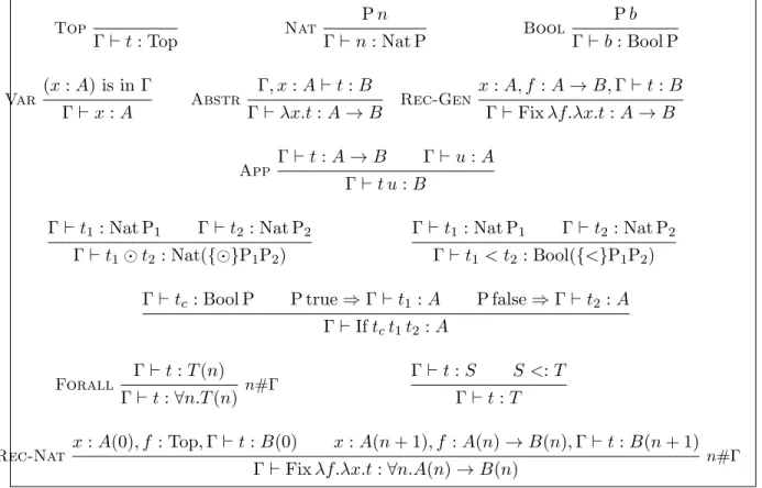
Our type system, presented in Table 4.1, is defined in two layers:

• A, B := Top | Nat PN | Bool PB | T → B where PN: N → Bool and PB : Bool → Bool

are predicates. • T := A | ∀n.T (n).

It has four main particularities:

• Top is the type of all terms. It is used for the typing rule Rec-Nat.

• Types Nat and Bool come with predicates, to specify more precisely inhabitants of these types. For example, we can use the predicate Peven := n 7→

(

true if n is even. false otherwise. to define the type Nat Peven of even numbers. We need such an expressive type system to

get an interesting theorem of operational correctness for our compiler.

• The quantification over naturals, which has to be seen as a restricted dependent type. Indeed, considering ∀n.T (n), the bounded variable n can only appear in the predicate of a type Nat or Bool. For example the type of the factorial function can be defined as : ∀n.Nat Pn→ Nat Pn!where Pk is the predicate x 7→ (x = k). This enables us to state

Top Γ ⊢ t : Top Nat P n Γ ⊢ n : Nat P Bool P b Γ ⊢ b : Bool P Var (x : A) is in Γ Γ ⊢ x : A Abstr Γ, x : A ⊢ t : B Γ ⊢ λx.t : A → B Rec-Gen x : A, f : A → B, Γ ⊢ t : B Γ ⊢ Fix λf.λx.t : A → B App Γ ⊢ t : A → B Γ ⊢ u : A Γ ⊢ t u : B Γ ⊢ t1 : Nat P1 Γ ⊢ t2: Nat P2 Γ ⊢ t1⊙ t2 : Nat({⊙}P1P2) Γ ⊢ t1 : Nat P1 Γ ⊢ t2 : Nat P2 Γ ⊢ t1< t2 : Bool({<}P1P2)

Γ ⊢ tc : Bool P P true ⇒ Γ ⊢ t1 : A P false ⇒ Γ ⊢ t2 : A

Γ ⊢ If tct1t2 : A

Forall Γ ⊢ t : T (n) Γ ⊢ t : ∀n.T (n) n#Γ

Γ ⊢ t : S S <: T Γ ⊢ t : T

Rec-Nat x : A(0), f : Top, Γ ⊢ t : B(0) x : A(n + 1), f : A(n) → B(n), Γ ⊢ t : B(n + 1)

Γ ⊢ Fix λf.λx.t : ∀n.A(n) → B(n) n#Γ

• For some technical reasons, we use a stratification on types, inspired by Hindley-Milner system, such that if we consider T → B, we have the guarantee that B does not contain quantified types. Indeed, as we will see later, kAk is closed by biorthogonal while it is not the case of k∀n.(T )k.

The typing rules presented in the Table 4.1 are standard. There is one particularity, the presence of two rules for the fixpoint operator, one general, Rec-Gen, and one restricted to the type Nat, Rec-Nat, which gives a quantified term and guarantees that the fixpoint is well-founded.

This means that when the typing proof of a term t does not use Rec-Gen, t normalizes. So we would like to get this crucial information down to compile t. To do so, we will see that ‚ can be defined as the set of processes which terminates. However, with this definition, it is not possible to deduce directly, from that fact that t is of type A, that compile t realizes A, as soon the typing of A use Rec-Gen. We will see later that step-indexing and divergence have to be used to solve this problem.

Finally, we use subtyping. The idea is to define a coercion of types, A <: B,

such that if we can prove that a term is of type B, then we can deduce it is of type A. This relation allows to instantiate quantifiers thanks to the following rule:

A(k) <: ∀n.A(n) for all k ∈ Nat.

Notice that polymorphic types can be handle in the same way than quantification on naturals.

4.2

The compiler

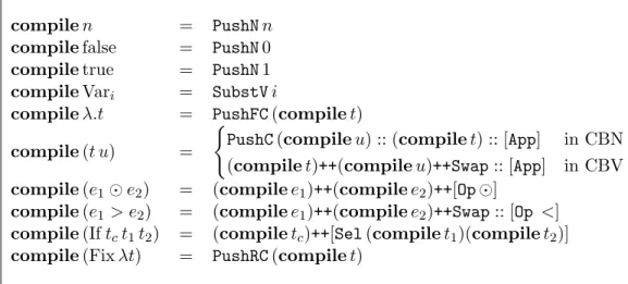
Now we will see how to generate code for SECD machines from λ-terms of our language. The compiler, presented in Table 4.2, is based on a modified version of our source language where variables have been replaced by De Bruijn indexes. Note that there are two definitions for the compilation of an application, depending on if we are in CBN or CBV.

compilen = PushNn compilefalse = PushN0 compiletrue = PushN1 compileVari = SubstVi

compileλ.t = PushFC(compile t) compile(t u) =

(

PushC(compile u) :: (compile t) :: [App] in CBN (compile t)++(compile u)++Swap :: [App] in CBV compile(e1⊙ e2) = (compile e1)++(compile e2)++[Op ⊙]

compile(e1 > e2) = (compile e1)++(compile e2)++Swap :: [Op <]

compile(If tct1t2) = (compile tc)++[Sel (compile t1)(compile t2)]

compile(Fix λt) = PushRC(compile t)

Chapter 5

Krivine realizability for SECD

We have seen that Krivine realizability for the KAM relies on the duality between closure and stack.

However, stacks of SECD machines does not have the same role as in KAM. Indeed, stacks in the KAM represents the arguments which will be consumed in the futur, while arguments are also stocked in the dump with the SECD.

For example, (λx.λy.t) u v will evaluate to t in front ofthe stack u · v with the KAM, while the compilation of this term to SECD with a CBV strategy gives the following code :

PushFC(compile t) :: compile u++[Swap, App]++compile v++[Swap, App]

and when the evaluation of compile u terminates, compile v++[Swap, App] will be put into the dump.

So tests should not be stacks anymore, but rather dumps, while realizers are values (and of course of thunk is a value so can be a realizer). And the interaction ⋆ between a value v and a dump d is defined in the following way: If v = C(c, e) (i.e. it is a thunk), then v ⋆ d = (c, e, [], d), otherwise v ⋆ d = ([], [], [v], d).

5.1

Step indexing

To deal with general recursion, we use the common technique of step indexing [3]. Indeed, when we want to prove the adequacy of the compiler by induction on the proof of Γ ⊢ t : A, the case of Rec-Gen is an issue, because evaluating compile λ.t interacting with a test of A → B, we get again compile λ.t interacting with a new test of A → B, so there seems to be no way to conclude. In the case of the well-founded rule Rec-Nat, we can make an induction on n, but for Rec-Gen there is nothing decreasing during the evaluation.

That is why realizers, tests and processes have to come with an index. But it is also the case of ‚: we consider a family of sets (‚i)i∈Nwhich have to be considered as approximations

of ‚.

And to deal with the basic case of the induction for Rec-Gen, we need to add a new axiom about ‚:

For example, if we want to take for ‚ the set of divergence terms, ‚i is simply the processes

which can reduce at least i times, and we see that ‚0 contains trivially all the processes.

When we forget about the Rec-Gen typing rule, we can simply take ‚i = ‚ for all i and

forget the axiom about ‚0.

5.2

Definition of tests

Realizers are couples formed by a value and an index, and the tests are couples formed by a dump and an index. Orthogonality relations between realizers and tests are defined as:

• (v, k) ⊥ (d, j) iff j ≤ k → v ⋆ d ∈ ‚j.

• (d, k) ⊥ (v, j) iff j ≤ k → v ⋆ d ∈ ‚j.

We will define the set of realizers of type A from the test of type A, by orthogonality: |A| = kAk⊥= {(v, k) ∈ Val × N | ∀(d, j) ∈ kAk , (v, k)⊥(d, j)}.

We write v A if for all k ∈ N, (v, k) A, and we will often abbreviate C(c, e) A to (c, e) A.

To define kAk, the set of tests of type A, we first need to define JAK, the set of primitive tests of type A :

• JTopK = {(d, k) ∈ Dump × N | ∀v ∈ Val, v ⋆ d ∈ ‚k}.

• JNat PK = {(d, k) ∈ Dump × N | ∀n ∈ N s.t. P n, (V n) ⋆ d ∈ ‚k}.

• JBool PK = {(d, k) ∈ Dump × N | ∀b ∈ B s.t. P b, (V ˆb) ⋆ d ∈ ‚k}.

• JA → BK = {(([App], [u], e) :: d, k) ∈ Dump × N | (u, k) ∈ |A| and ∀j ≤ k, (d, j) ∈ kBk}. But the definition of these primitive tests is too rigid, we would like to be able to define tests which “behave” extensionally like them. More precisely, if d is a test of T and for all value u, d ⋆ u ∈ ‚ implies d′

⋆ u ∈ ‚, we would like d′

be also a test of T . That is why one has to close these sets by biorthogonality, to get more tests:

kAk = JAK⊥⊥.

Notice that we close the sets only for non quantified types. Indeed, we define tests of ∀n.T (n) in the following way:

k∀n.T (n)k = [

n∈N

kT (n)k .

This is where are stratified definition of types comes into the picture. We know that every type defined in the first layer is closed by biorthogonality.

Unwinding the biorthogonality (and forgetting for one moment step-indexing), we get that d is a test of type A if it goes well with all the values v which go well with the primitives tests of type A.

However, since we have expended SECD machine with thunks, we must keep in mind that we also expended tests, which could use its.

This could be a problem when we want to prove the correction of the CBV compiler, so in this case we need to restrict the definition of biorthogonality to values which are not thunks: d is a test of type A if it goes well with all the values v which are not thunks and go well with the primitives tests of type A. This definition is also fine to prove the correction of the CBN compiler.

Notice that we do not change the definition of orthogonality used between realizers and tests. Indeed, to prove the adequacy lemma, we use the fact that if t is of type A then C(compile t, []) A.

Finally, we can prove the adequacy lemma between type system and realizability:

Theorem 5(Adequacy). if Γ ⊢ t : T then for all environments e such that e⊲Γ, (compile t, e) T .

We sketch now the demonstration of this important lemma. It is made by induction on the proof of Γ ⊢ t : T . Here are some induction cases, represented by the different typing rules.

Nat _{: Let d ∈ kNat Pk, then (PushN n, e, [], d) ≻ ([], e, [V(n)], d) ∈ ‚ and we can conclude} since ‚ is closed by anti-reduction.

Var : Let d ∈ kAk then (SubstV n, e, [], d) ≻ u ⋆ d where u is the nth element of e, and by definition of e ⊲ Γ, u A so u⊥d.

Abstr : Let d ∈ kAk then (PushFC c, e, [], d) ≻ ([], e, [FC(c, e)], d). Unfolding biorthogonality, we know that u ⋆ d ∈ ‚ for all u ∈ Val such that for all primitive tests d′

, u⊥d′

. So if we prove that for all primitive tests d ∈ JA → BK, ([], e, [FC(c, e)], d) ∈ ‚, then we will get what we want. But d = ([App], u, e) :: d′

with u A and d′

∈ kBk and ([], e, [FC(c, e)], [App], u, e) :: d′

) ≻2 (c, u :: e, [], d′

) and by induction hypothesis (c, u :: e) B since u :: e ⊲ A, Γ.

App : Here we have to split the proof in two parts, one for the CBN evaluation strategy and one for the CBV :

CBN : (PushC (compile u) :: (compile t) :: [App], e, [], d) ≻ (compile t :: [App], e, C(compile u, e), d) then we use the fact that if (compile t, e, ([App], C(compile u, e), e) :: d) ∈ ‚ then

(compile t :: [App], e, C(compile u, e), d) ∈ ‚ to conclude.

CBV : Here again, we use the fact that if (compile t, e, [], ((compile u)++Swap :: [App], e, []) :: d) ∈ ‚ then ((compile t)++(compile u)++Swap :: [App], e, [], d) ∈ ‚. Then, us-ing the extentionality property of kAk we get by biorthogonality, we prove that ((compile u)++Swap :: [App], e, []) :: d is a test of A → B when d is a test of B.

Chapter 6

Results of correctness

Once we have proved that (c, e) T , properties on c can be deduced, in the same way we have done with the KAM. We first restrict to the case where Γ ⊢ t : T is proved without Rec-Gen_{. Then we are sure that t normalizes, and we can work with ‚ as the set of the} processes reducing to ([], e, [v], []) for some v ∈ Val. In this case, we can forget everything about step-indexing.

In what follows, we will suppose that predicates P which come from types Nat and Bool are expressible with SECD machines. More precisely, NatP is expressible iff there exists a code c such that for all c′

∈ Code, v ∈ Val and d ∈ Dump, if v satisfies P then (c++c′

, [], [v], d) is evaluated to (c++c′

, [], [V(1)], d), otherwise it is evaluated to (c++c′

, [], [V(0)], d). This is of course the case of Pn.

Then we can prove the following correctness theorem:

Theorem 6 (Operational correctness). If Γ ⊢ t : T and e ⊲ Γ then (compile t, e, [], []) ≻∗

([], e′

, [v], []) and v is a value of type T : • If T is Nat P then v = V(n) and P(n).

• If T is Bool P then v = V(b) with b = 0 or b = 1 and P(b)

• If T is S → B then v = FC(c, e) or v = RC(c, e) and for all values u ⊢ S, (App, [], v :: [u], []) ≻∗

([], e′

, [w], []) with w of type B.

• If T is ∀n.S(n) then for all n ∈ N, v is a value of type S(n).

This theorem gives us operational results for types Nat Pn or Bool Pb. Indeed, in these

cases, t →∗

n so the reduction of t corresponds to the evaluation of compile t.

We will prove a more general result about closure (c, e) T , then operational correctness follows from adequacy lemma. First, as what we did for the KAM, considering the interaction u ⋆ d (in particular for u = C(c, e)), we prove that the test d is evaluated:

if u ⋆ d ≻n_{([], e, [v], []) then there exists k ≤ n s.t. u ⋆ d ≻}k_{([], e}′

, [v′

], d). Then, we make an induction on T :

• if T = Nat P, one has to prove that (c, e, [], []) ≻∗

([], e′

, [V(m)], []) with m satisfying P. Taking d ∈ kNat Pk, we already know that:

– (c, e, [], d) ≻∗

([], e, [v′

], d). – ([], [], [V(n)], d) ≻∗

([], e′

, [w], []) for all n satisfying P.

So we need to be able to pick up a test d which could discriminate between V(n) and other values. To do so, the predicate P needs to be expressible in our language. For example, taking P as Pn, d can be (PushV n :: EqTest :: [Sel [PushV 1] Ω], [], []) where Ω

is a diverging term. Then ([], e, [v′

], d) ≻2 _{(EqTest :: [Sel [PushV 1] Ω], [], V(n) :: [v}′

], []) ≻∗ ( ([], [], [V(1)], []) ∈ ‚ if v′ = V(n). (Ω, [], s, []) /∈ ‚ otherwise. Using the fact that ([], e, [v′

], d) ∈ ‚,it cannot reduce to a process not in ‚, so v′

= V(n). The proof for Bool P is made in the same way.

• If (c, e) S → B and u S, we first prove that (c, e, [], [] ≻∗ _{([], e, [v], []) using the}

fact that the empty dump is a valid test. Then for all u S one has to prove that ([App], e, v :: [u], []) ≻∗

([], e′

, [w], []) and w B.

To do so, one takes a test d in kBk, then ([App], e, [u]) :: d is in kA → Bk so ([], [], [v], ([App], e, [u]) :: d) ≻ ([App], e, v :: [u], d) ≻∗ ([], e′, [w], d)

So v has to be FC(c, env) or RC(c, env), and w ⊥ d for all d ∈ kBk, i.e. w B.

• Finally, if (c, e) ∀n.S(n), it satisfies for all n ∈ N the tests in kS(n)k, i.e. (c, e) S(n). Note when S(n) is U (n) → B(n), we get an uniform result of correctness : for all n ∈ N and u A(n), (c++[App], e, [u], []) ≻∗

([], e′

, [v], []) with v B.

Notice that the informations we get on compile t are strictly those we get from the typing of A. So if we cannot deduce that t normalizes from its type, for example if the proof of its typing use Rec-Gen, then their is no way we can get with this method that the evaluation of compile t terminates. But in this case, we can still get some information on the result of the evaluation of compile t, if we suppose it terminates. Indeed, taking ‚ as the diverging processes and using step-indexing just as explain above, tests interacting with compile t must be evaluated since compile t terminates. And it is still possible to build tests which discriminate between a natural number and an other value, but here the case where it must diverge is swapped.

6.1

The example of Factorial

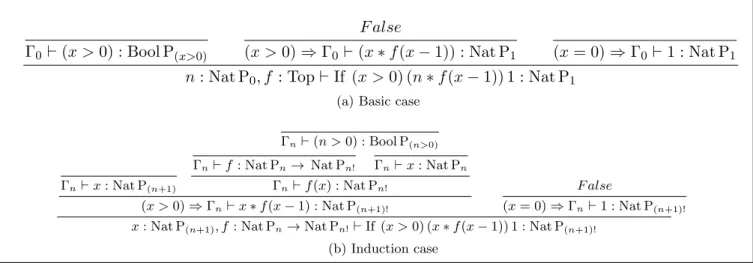
Consider the term Fac = Fix (λf.λn.(If (n > 0) (n ∗ f (n − 1)) 1)) which computes the factorial of a natural number. Then, as shown in the table 6.1, it can be typed using Rec-Nat. The type we get is

Γ0 ⊢ (x > 0) : Bool P(x>0)

F alse

(x > 0) ⇒ Γ0 ⊢ (x ∗ f (x − 1)) : Nat P1 (x = 0) ⇒ Γ0 ⊢ 1 : Nat P1

n : Nat P0, f : Top ⊢ If (x > 0) (n ∗ f (x − 1)) 1 : Nat P1

(a) Basic case Γn⊢(n > 0) : Bool P(n>0)

Γn⊢x: Nat P(n+1)

Γn⊢f: Nat Pn→ Nat Pn! Γn⊢x: Nat Pn

Γn⊢f(x) : Nat Pn!

(x > 0) ⇒ Γn⊢x ∗ f(x − 1) : Nat P(n+1)!

F alse

(x = 0) ⇒ Γn⊢1 : Nat P(n+1)!

x: Nat P(n+1), f: Nat Pn→Nat Pn!⊢If (x > 0) (x ∗ f (x − 1)) 1 : Nat P(n+1)!

(b) Induction case Table 6.1: Typing of Factorial

which is the more precise we can hope. So for all values v which realize Nat Pn, (compile Fac, [], [v], [])

realizes Nat Pn!. But then, for all n ∈ Nat,

(compile Fac, [], [V(n)], []) ≻∗ ([], e, [V(n)], []), which is a special case of our operational correctness of our compiler.

Chapter 7

Realizability for a language with

references

Now, we try to add some imperative features to our source language, namely mutable states. To do so, we follow what is done in CaML, so we suppose that we work now with CBV strategy.

We add to our language five new terms :

• () which represents the unit value, i.e. the result of a computation which only works on references.

• t; u, the usual sequencing operation which evaluate first t, then u. Note that t should evaluate to ().

• ref t which creates a reference with t stocked inside and reduce to the address of this reference.

• !t which gives the value the reference that t points to contains.

• t := u which modify the reference t points to, to put u inside, and return (), the unit value.

We also need to add addresses of references to our languages, which lies on the set Addr. The reduction must remember where references are stocked and what they contains. To do so, a term comes with a partial function h : Addr ⇀ Value, and the reduction is then defined by :

• (ref v, h) → (i, h′

) with h′

(k) = (

v if k = i

h(k) otherwise. and i is a fresh address. • (!i, h) → (h(i), h). • (t := v, h) → ((), h′ ) with h′ (k) = ( v if k = i h(k) otherwise.

We also have to extend the type system to be able to give a type to ref t. To do so, we introduce for each type A a type ref A which represents the type of the addresses which contain a value of type A.

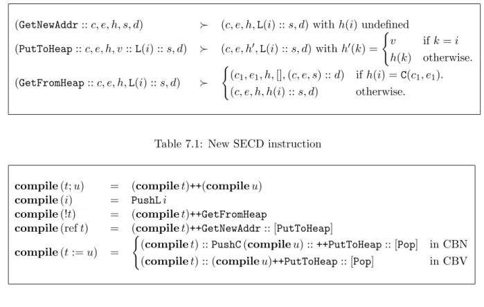
(GetNewAddr :: c, e, h, s, d) ≻ (c, e, h, L(i) :: s, d) with h(i) undefined (PutToHeap :: c, e, h, v :: L(i) :: s, d) ≻ (c, e, h′ , L(i) :: s, d) with h′ (k) = ( v if k = i h(k) otherwise. (GetFromHeap :: c, e, h, L(i) :: s, d) ≻ ( (c1, e1, h, [], (c, e, s) :: d) if h(i) = C(c1, e1). (c, e, h, h(i) :: s, d) otherwise.

Table 7.1: New SECD instruction

compile(t; u) = (compile t)++(compile u) compile(i) = PushLi

compile(!t) = (compile t)++GetFromHeap

compile(ref t) = (compile t)++GetNewAddr :: [PutToHeap] compile(t := u) =

(

(compile t) :: PushC (compile u) :: ++PutToHeap :: [Pop] in CBN (compile t) :: (compile u)++PutToHeap :: [Pop] in CBV

Table 7.2: The compiler for references

Then, we extend SECD machine to be able to compile our extended language. We add a

heap to them, represented by a partial function h : N ⇀ Val, and three new instructions :

• GetNewAddr which gives a fresh address in the heap.

• PutToHeap which put in the heap, at the address which is on the top of the stack the value just below.

• GetFromHeap which gives the value in the heap located in the address which is on the top of the stack.

We also add addresses of heap as new values, noted L(i).

Now we need to define our typing rules, and see how to define tests such that we get an adequacy lemma, but also a useful correction theorem.

7.1

A first attempt : ML like typing

Type judgments come with an usual typing context Γ plus a typing function of heap Υ, represented by a partial function Addr ⇀ Type.

Heap Υ(i) = A

Υ, Γ ⊢ i : ref A Deref

Υ, Γ ⊢ t : ref A Υ, Γ ⊢!t : A

Ref Υ, Γ ⊢ t : A

Υ, Γ ⊢ ref t : ref A ModRef

Υ, Γ ⊢ t : ref A Υ, Γ ⊢ u : A Υ, Γ ⊢ t := u : Unit

We need to define what a test of ref A is. The idea is to test if what we read in the address is a value of type A, but also if it is possible to write a value of type A in the heap in this address. So tests is simply the union of these two possibilities :

Jref AK = {([GetFromHeap], [], []) :: d) s.t. d ∈ kAk}

∪ {(PutToHeap :: [Pop], [u], []) :: d, k) s.t. ∀h ∈ Heap(u, h, k) ∈ |A| and (d, k) ∈ kUnitk} Then, one can extend the adequacy lemma to this language. To do so, we first define, just

like for typing context, a compatibility relation between an heap h and a typing function of heap Υ, still noted h ⊲ Υ and defined by :

h ⊲ Γ iff they have the same domain of definition and for all i in this domain, h(i) Υ(i). The adequacy lemma is simply :

Theorem 7 (Adequacy). if Υ, Γ ⊢ t : T then for all environments e such that e ⊲ Γ and for

all heap h such that h ⊲ Υ (compile t, e, h) T .

Here are the proof for some of the new typing rules :

Heap _{: Let d ∈ kref Ak, then (PushL i, e, h, [], d) ≻ ([], e, h, [L(i)], d) and indeed (h(i), h) A} and we can put in h(i) a new value which realizes A since we still keep that the new heap h′

⊲ Υ.

Deref : Let d ∈ kAk, then by induction hypothesis (compile t, e, h)⊥([GetFromHeap], [], []) :: d) so (compile t++[GetFromHeap], e, h)⊥d.

The main problem with this type system is that it is impossible to change the value of a reference to a value of a different type. So a reference of type ref NatPn could only contain

n, so references are in this case not really mutable.

7.2

A second one : Hoare typing

To solve this issue, we need to allow type-varying modifications of references. But this implies that the evaluation of a term will modify the heap typing function Υ, so we need to show the evolution of this function in the typing rules. the fact that t is of type A with the typing context Γ, and modify the heap typing function Υ to Υ′

is noted : Γ ⊢ {Υ}t : A{Υ′

This is made by analogy with Hoare semantics, where we specify preconditions and postcon-dition about memory to prove a property.

However, a problem appears with terms like t := u when t is not an address, or ref t, since it is no more possible to state the modification of Υ since we do not know, before the execution of the term, which address will be modified or allocated.

A solution is to forbid these terms. The only possibility to get or modified a reference is to give explicitly its address. One can see this restricted language as an intermediate step between our high-level language and SECD machine, which could has been generated by the first pass of our compiler.

With this restriction, we are now able to give our typing rules : Seq Γ ⊢ {Υ}t : Unit{Υ

′

} Γ ⊢ {Υ′}u : A{Υ′′} Γ ⊢ {Υ}t; u : A{Υ′′}

Heap Υ(i) = A

Γ ⊢ {Υ}i : ref A{Υ} Deref

Υ(i) = A Γ ⊢ {Υ}!i : A{Υ}

ModRef Υ(i) = A Γ ⊢ {Υ}u : B{Υ

′

} A ≃ B

Γ ⊢ {Υ}i := u : Unit{Υ′′} with Υ′′(j) = (

B if j = i Υ′

(j) otherwise. The realizability relation, just like tests, depends now on the heap typing function :

(u, h) ΥT iff for all d ∈ kT kΥ, (u, h) ⋆ d ∈ ‚

.

Now we define primitive tests :

• JTopK_Υ = {d ∈ Dump | ∀v ∈ Val, ∀h ∈ Heap s.t. h ⊲ Υ, v ⋆ d ∈ ‚}.

• JUnitK_Υ= {d ∈ Dump | ∀e ∈ Env, ∀h ∈ Heap s.t. h ⊲ Υ, ([], e, h, [], d) ∈ ‚}. • JNat PK_Υ = {d ∈ Dump | ∀n ∈ N s.t. P n, ∀h ∈ Heap s.t. h ⊲ Υ, (V n, h) ⋆ d ∈ ‚}. • JBool PK_Υ = {d ∈ Dump | ∀b ∈ B s.t. P b, ∀h ∈ Heap s.t. h ⊲ Υ, (V ˆb, h) ⋆ d ∈ ‚}.

• JA → BK_Υ = {(([App], [u], e) :: d) ∈ Dump | ∀h ∈ Heap s.t. h ⊲ Υ, (u, h) ∈ |A|_Υ, d ∈ kBk_Υ}.

• Jref AK_Υ= {([GetFromHeap], [], []) :: d) s.t. d ∈ kAk_Υ}.

Compared to the previous definition of Jref AK, only the access and not the writing is tested here. Indeed, there is no more restriction on what a reference can contains so it is no more useful to test writing to prove the adequacy lemma.

Theorem 8 (Adequacy). if Γ ⊢ {Υ}t : T {Υ′

} then for all environments e and heaps h such

Seq _{: If (compile t, e, h) Υ}′ Unit and (compile u, e, h′) _Υ′′ A with h′ ⊲ Υ′ then we just

have to show that for all d ∈ kAk_Υ′′, (compile u, e, []) :: d is in kUnitk_Υ, which is direct.

Heap _{: If (Υ(i), h) A and d ∈ kAk, then (PushL i, e, h, [], (GetFromHeap, [], []) :: d) ≻}2 (GetFromHeap, e, h, L(i), d) ≻ (h(i), h) ⋆ d) so we can conclude easily.

Deref : (PushL i :: GetFromHeap, e, h, [], d) is equivalent to ([PushL i], e, h, [], (GetFromHeap, e, []) :: d) so the proof is the same than for Heap.

ModRef :

CBV : Taking d ∈ kUnitk we prove that d′

= (PutToHeap :: [Pop], e, [L(i)]) :: d is a test of A.

CBN This case is direct since (PushL i :: PushC (compile t) :: PutToHeap :: [Pop], e, h, [], d) ≻ ([], e, h′

Chapter 8

Discussion and Future work

We have seen how the correctness of our compiler can be deduced from the usual adequacy lemma of realizability. But this result of correctness has to be seen as a result of conservation of typing between our high-level term and its compiled program.

It does not link the reduction of a term in the source language with the evaluation of it compiled term. Indeed, we haven’t even defined the reduction of our source language. But it is still possible to get some operational results, as soon as our type system is rich enough to give precise information on the reduction of high-level terms.

More precisely, a global operational correspondence between high-level and low-level lan-guage, abstract from the type system, can be obtain thanks to four results :

• A subject reduction theorem which links typing and operational reduction of the high level language : If Γ ⊢ t : A and t → u then Γ ⊢ u : A. Combined with a termination property, we get that t reduces to a value v of type A. And if A is precise enough (like NatPn) then v is unique (for example n).

• A expressiveness theorem about type system which characterizes the terms which are typeable, even if the type system is undecidable, which is of course the case with the one we used here. For example, typeable terms of System T are exactly those we can prove the termination in Peano Arithmetic. It should be possible to get a similar result for our type system.

• An adequacy theorem which links types of the high level language with low-level pro-grams.

• A correctness result which specifies the behavior of low-level programs, depending on which type they realize.

Concerning the formalization in Coq of this work, it is interesting to see that the adequacy lemma takes less than 500 lines of code to be proved. The most difficult part is in fact some reduction correspondences which allow to transfert code from Code to Dump.

This work has to be seen as a first step to a well more ambitious program to prove correctness of a compiler for a richer high-level language to real assembly code. Here are some extension we plan to tackle

8.1

Dealing with imperative features

Our treatment of mutable states is not completely satisfactory, not because it is hard to define realizability for it, but because it is hard to get a type system which allows type-varying modification.

Hoare Type Theory [14] seems to be the ideal candidate to do so. Indeed, it shares many features with our type system, like predicates to describe precisely the result the program could return, or a clear distinction between terminating and possibly diverging computation. But it also gives a fine control of memory, taking ideas from separation logic.

An other approach would be to represent effects with monads, like in Haskell. Then, we could extend the KAM in a monadic way, using ideas from [1]. An interesting challenge would try to find a way to define tests for the most common monads.

For example, considering the State monad, we could image define a test of State A from a test d of A, adding the possibility for d to use functions get and put.

8.2

Compiling to a lower level language

SECD machine is a first step to assembly language. Indeed, dumps can be seen as a way to save the code pointer plus the current environment and stack. But it is not straight to extend this method so that realizers could be assembly terms, for many reasons: (1) an assembly program is almighty and can cheat when interacting with a test, simply erasing it and faking it has succeeded it, (2) we need to deal with memory allocation. (3) There is no more App instruction, tests of A → B cannot be defined directly anymore.

But it seems doable to adapt our framework to the work of [7] . Tests would then become general context, the hole would not have to always be in head position.

8.3

A richer type system

Type system is the key point of our work, so the more expressive it is the more correctness results will be interesting.

We already talk about typing of imperative effects, but we could also imagine adding features like polymorphism or inductive types. Polymorphism should be easy to add, since it can be handle in the same way the universal quantification on natural numbers has been done, with some restriction a la Hindley-Milner.

We could follow [4] to deal with inductive types. Indeed, we have already step-indexing in our realizability definitions so their method seems to be doable in our framework.

Finally, type systems could also be useful to control complexity of programs. Indeed, system derived from linear logic, like Light Linear Logic or Elementary Linear Logic, has shown their power to give precise account on complexity Some works have been made on realizability for this kind of type systems, and we could imagine using them to prove property of complexity conservation for compiler. This means that if we prove that a high-level program has an

asymptotic execution time in f (n) where n is the input size, then the compiled program would also be executed asymptotically in f (n).

8.4

Equivalence of programs

To conclude, an interesting question is to see what equivalence relation the realizability gives us. Indeed, define u ≃Au′ iff for all d ∈ kAk , u⊥d iff u′⊥d.

Then we get some interesting equivalence, like compile (u + v) ≃Natcompile(v + u). But

we need to work with this typed relation. Indeed, defining u ≃Au′ iff for all dump d, u⊥d iff

u′

⊥d, we could not prove easily anymore compile (u + v) ≃Natcompile(v + u).

More generally, a question we wish to tackle is the relation between contextual equivalence of the high-level language and this equivalence relation ≃A.

Bibliography

[1] M.S. Ager, O. Danvy, and J. Midtgaard. A functional correspondence between monadic evaluators and abstract machines for languages with computational effects. Theoretical

Computer Science, 342(1):149–172, 2005.

[2] A. Appel. Foundational proof-carrying code. In Proc. 16th IEEE Symposium on Logic

in Computer Science (LICS), 2001.

[3] A. Appel and D. McAllester. An indexed model of recursive types for foundational proof-carrying code. ACM Transactions on Programming Languages and Systems (TOPLAS), 23(5), 2001.

[4] A.W. Appel, P.-A. Melli`es, C.D. Richards, and J. Vouillon. A very modal model of a modern, major, general type system. Proceedings of the 34th annual ACM

SIGPLAN-SIGACT symposium on Principles of programming languages, pages 109–122, 2007.

[5] N. Benton. Abstracting allocation: The new new thing. In CSL ’06, volume 4207 of

LNCS. Springer-Verlag, September 2006.

[6] Nick Benton and Chung-Kil Hur. Biorthogonality, step-indexing and compiler correct-ness. In ICFP ’09: Proceedings of the 14th ACM SIGPLAN international conference on

Functional programming, pages 97–108, New York, NY, USA, 2009. ACM.

[7] Nick Benton and Nicolas Tabareau. Compiling functional types to relational specifications for low level imperative code. In TLDI ’09: Proceedings of the 4th international workshop

on Types in language design and implementation, pages 3–14, New York, NY, USA, 2009.

ACM.

[8] M. Dave. Compiler verification: a bibliography. ACM SIGSOFT Software Engineering

Notes, 28(6), 2003.

[9] G. Kreisel. Interpretation of analysis by means of constructive functionals of finite types.

Constructivity in mathematics, pages 101–128, 1959.

[10] JL Krivine. Realizability in classical logic. Course notes of a series of lectures given in the University of Marseille, may 2004 (last revision: july 2005). Panoramas et syntheses,

Soci´et´e Math´ematique de France.

[11] PJ Landin. The mechanical evaluation of expressions. The Computer Journal, 6(4):308, 1964.

[12] X. Leroy. Formal certification of a compiler back-end, or: programming a compiler with a proof assistant. In Proc. 33rd Symposium on Principles of Programming Languages

(POPL), 2006.

[13] J. McCarthy and J. Painter. Correctness of a Compiler for Arithmetic Expressions.

Proceedings Symposium in Applied Mathematics, 19:33–41, 1967.

[14] A. Nanevski, G. Morrisett, and L. Birkedal. Polymorphism and separation in hoare type theory. In Proceedings of the eleventh ACM SIGPLAN international conference on

Functional programming, page 73. ACM, 2006.

[15] J. Van Oosten. Realizability: a historical essay. Mathematical Structures in Computer