Anthropogenic pressures and Bay of Biscay nurseries: identification, spatial
variations and synthetize representation
Par : Solène MORA
Soutenu à Rennes le 12 septembre 2018 Devant le jury composé de :
Président : Jérôme GUITTON, Agrocampus Ouest Maîtres de stage :
Anik BRIND'AMOUR, Ifremer Nantes Aourell Mauffret, Ifremer Nantes Hervé LE BRIS, Agrocampus Ouest
Enseignant référent : Olivier LE PAPE, Agrocampus Ouest
Autres membres du jury (Nom, Qualité) Jérémy LOBRY, IRSTEA
Les analyses et les conclusions de ce travail d'étudiant n'engagent que la responsabilité de son auteur et non celle d’AGROCAMPUS OUEST
AGROCAMPUS OUEST Année universitaire : 2017-2018 Spécialité : Ingénieur agronome Spécialisation (et option éventuelle) : Sciences halieutiques et aquacoles
(Ressources et Ecosystèmes Aquatiques)
Mémoire de Fin d'Études
CFR Angers CFR Rennes
d’Ingénieur de l’Institut Supérieur des Sciences agronomiques, agroalimentaires, horticoles et du paysage
de Master de l’Institut Supérieur des Sciences agronomiques, agroalimentaires, horticoles et du paysage
d'un autre établissement (étudiant arrivé en M2)
Ce document est soumis aux conditions d’utilisation
«Paternité-Pas d'Utilisation Commerciale-Pas de Modification 4.0 France»
disponible en ligne http://creativecommons.org/licenses/by-nc-nd/4.0/deed.fr
Introduction – Contamination – Pêche –
Remercîments
Je tiens à remercier mes trois encadrants de stage Anik brind’Amour, Aourell Mauffret et Hervé Le Bris pour leur aide, leurs précieux conseils et le temps qu’ils m’ont accordé pendant ces six mois. Je remercie tout particulièrement Hervé et Anik pour leur soutien et leur aide pour cette fin de stage très chargée.
Je tenais également à remercier les deux équipes qui m’ont accueilli aussi bien à l’Ifremer Nantes qu’à l’Agrocampus. Ainsi que toutes les personnes qui m’ont aidé lors de ce stage.
Enfin, merci à ma famille et à tous ceux qui m’ont soutenu durant ce stage et plus particulièrement à ma collègue de bureau Auriane pour avoir été là et attentive dans cette dernière ligne droite.
Résumé étendu en français
Pressions anthropiques et nourriceries du golfe de Gascogne : identification, variations spatiales et représentation synthétique
Contexte
Les écosystèmes côtiers et estuariens comptent parmi les écosystèmes les plus productifs de la planète ayant une valeur écologique mais aussi économique importante. Ils assurent de multiples rôles, comme celui de nourriceries pour les juvéniles de nombreuses espèces marines. Mais ces écosystèmes subissent également de multiples pressions issues d’activités d’origine anthropique. Ces impacts peuvent être causés de manière directe par les activités de pêche, d’extraction de granulat, de clapage ou dus à des activités terrestres affectant par ruissellement les zones côtières. A cela s’ajoutent des pressions indirectes liées aux changements climatiques. Ces pressions vont modifier à l’échelle des populations, leur recrutement, leur croissance et leur abondance mais également à l’échelle des communautés, la biodiversité, la structure et le fonctionnement trophique.
Dans cette étude nous distinguons l’activité des pressions qu’elle engendre. Une pression est définie comme le mécanisme par lequel l’activité influence le milieu. Il est important de noter qu’une activité peut engendrer plusieurs pressions sur le milieu et qu’une pression peut être causée par plusieurs activités.
La compréhension des effets des pressions anthropiques sur les communautés marines nécessite de bien identifier, voire quantifier, les activités humaines et les pressions qu'elles engendrent. Une méthode pour quantifier ces pressions passe par la construction d’un indicateur global de pression. Cela permet de synthétiser les pressions anthropiques exercées, de les cartographier, de les classer et de comparer les différentes zones étudiées. Cela peut également être une aide à la décision pour la gestion intégrée des zones côtières.
Dans le cadre de la DCE (Directive Cadre sur l’Eau), un indicateur de pressions anthropiques a ainsi été établi en France mais il porte uniquement sur les eaux de transitions (estuaires et lagunes). Il y a donc un réel enjeu à étudier les pressions que subissent les nourriceries côtières. Notre étude vient compléter et continuer le travail commencé par Saulnier et al, (2017) et porte sur les six zones de nourriceries dans le golfe de Gascogne, identifiées lors de précédentes études.
Pour cette étude l’année 2014 a été sélectionnée comme année de référence pour évaluer l’impact des pressions anthropiques sur les nourriceries du golfe de Gascogne.
Objectifs
L’objectif de cette étude est donc d’identifier et quantifier les pressions anthropiques s’appliquant sur ces six zones de nourriceries et d’analyser leurs différences par la construction d’un indicateur de pression permettant d’estimer d’une part le niveau global de pression de chaque nourricerie et d'autre part, d'identifier les zones à forts enjeux anthropiques en cartographiant l’indicateur à l'échelle d'une nourricerie. Deux jeux de données (contamination chimique et pêche) seront notamment travaillés pour pouvoir inclure au mieux ces pressions dans notre étude.
Matériel et Méthode
Cinq pressions ont été retenues pour cette étude : l’extraction de granulat, la présence d’une espèce invasive (Crepidula Fornicata), le clapage, la pêche et la contamination chimique. Les trois dernières ont été plus particulièrement travaillées.
Les données de contamination ont été qualifiées, standardisées et normalisées. Deux ACP distincts ont été réalisés sur les métaux et les composés organiques. Les coordonnées sur le 1er axe ont été utilisées comme indicateur de contamination. Une extension spatiale de type buffer leur a ensuite été appliquée afin de représenter la réelle dispersion spatiale de la pression de contamination depuis le centre des estuaires.
Cette extension spatiale a également été appliquée aux points de clapage qui sans cette extension traduisent une pression appliquée aléatoirement en un point de la zone de clapage.
Les données de pêche sont issues de plusieurs jeux de données qui ont été travaillés afin de reconstituer le nombre de sorties des bateaux côtiers dans le golfe de Gascogne en 2014.
Les données des cinq pressions ont été transformées en indices et standardisées avant d’être incluses dans un indicateur global de pression.
Résultat et discussion
Notre étude avait pour but d’identifier, voire de quantifier, et synthétiser les pressions anthropiques s’appliquant sur les six zones de nourriceries du Golfe de Gascogne. Une grande part du travail a été investie pour développer un cadre méthodologique impliquant un travail conséquent concernant la sélection et le traitement des données. Dans le temps imparti nous avons réussi à proposer une approche basée sur des données âprement sélectionnées. Cette démarche a permis de livrer des premiers résultats. Un premier indicateur global de pression a été construit pour chaque nourricerie. Le niveau global de chaque pression a également été étudié dans chaque nourricerie. Les pressions de contamination et de pêche sont prépondérantes en termes de surfaces impactées et dans la contribution à l’indicateur global de pression. La Gironde et la baie de Bourgneuf apparaissent comme les deux zones les plus touchées par les cinq pressions sélectionnées. Le pertuis breton s’illustre quant à lui, en plus d’être la nourricerie la moins touchée comme étant la seule nourricerie où la pression dominante est la pêche.
Ces résultats sont cependant à nuancer au vu des choix effectués concernant les données, et les hypothèses de travail requises. Une étude de sensibilité devra également être conduite concernant la technique de spatialisation des données utilisée ainsi que la pondération des pressions dans l’indicateur. Les résultats de l’indicateur global doivent également être complétés par un indicateur spatialisé qui permettra d’évaluer les différences de répartition des pressions cumulées à l’intérieur d’une nourricerie.
Table of Contents
INTRODUCTION ... 1 1.
MATERIEL AND METHODS ... 3 2.
2.1. Study sites ... 3 2.2. Pressure selection and detailed information on contamination and fishing
pressures ... 4
2.2.1. Chemical contamination pressure 5
2.2.2 Fishing activity in the Bay of Biscay 8
2.2.3 Aggregate extraction 9
2.2.4 Piling 9
2.2.5 Invasive species 10
2.3. Spatial extension of source and diffuse pressures: the case of chemical contamination and piling ... 10 2.4. Computation of the multimetric pressure index... 12 2.4.1. Building activities index and the contamination pressure index 12
2.4.2. Building the multimetric indicator 13
2.5. Data processing ... 14 RESULTS ... 15 3.
3.1. Chemical contamination ... 15 3.2. Fishing activity in the coastal part of the Bay of Biscay ... 16 3.2.1. General decrease of the fishing fleet in the Bay of Biscay 16
3.2.2. Representativeness of aerial surveys data 17
3.2.3. Investigating work hypothesis 18
3.2.4. Reconstitution of the evolution of the fleets operating in the Bay of
Biscay 19
3.2.5. Assessing the temporal evolution of the coastal fleets by region 20 3.3 Spatialization of data points for chemical contamination and piling ... 22
Buffers on pilling points sources impact 23
3.4 Studying contrasts between nurseries: application of the multimetric pressure indicator to the nurseries sites in the Bay of Biscay ... 23 3.4.1. Contribution of the different anthropogenic pressures to the multimetric
indicator 24
DISCUSSION ... 26 4.
4.1. Limitations of the study and methodological choices... 26
4.1.1 Chemical contamination 26
4.2.2 Fishing index 27
4.1.3 Other pressures 28
4.2 Possible improvements to the approach and prospects ... 28 REFERENCES ... 30 5.
APPENDICES ... 34 6.
List of figures
Figure 1. Location of the studied nurseries of the Bay of Biscay... 3 Figure 2. Location of sampling stations for both biota and sediment matrices for metal (left)
and organic (right) compounds ... 5 Figure 3. Correlation circles for metals (A) and organic compounds (B) ... 15 Figure 4. Repartition of individuals depending of the nursery for metals (A) and organic (B)
compounds ... 15 Figure 5. Evolution of vessels repartition depending on their length in the Bay of Biscay (A)
and mean repartition of the coastal fleet (B) (data extract from SIH syntheses) ... 16 Figure 6. Comparison of the number of fishing trips between aerial surveys and SIH data for
the year 2001 ... 17 Figure 7. Stacked area graph of regional contribution to the coastal fleet between 2003 and
2016 ... 18 Figure 8. Evolution of the Bay of Biscay coastal fleet from 2001 to 2014 using both SIH data
sets at the scale of the bay (A) and at the regional scale (B, C, D,E) ... 19 Figure 9. Linear regressions on SIH data extract from the syntheses ... 20 Figure 10. Geographic positions of coastal vessels reconstituted for 2014 (A) and pressure
index due to fishing activity (B) ... 21 Figure 11. Result of the spatialization of pressure index for metal contamination (A) and
organic contamination (B) ... 22 Figure 12. Spatialization of the piling index ... 23 Figure 13. Boxplot of the standardize pressure indices ... 23 Figure 14. Global Pressure Indices (GPI) and Average Level of Pressure (ALP) for each
nursery ... 25 Figure 15. Distribution of dissolved metals (µg/l) as a function of salinity for the Seine estuary
(Chiffoleau et al., 2001) ... 43
List of Tables
Table 1. Nature, temporal and spatial extension, final data used in the indicator and data sources. ... 4 Table 2. Buffers parameters ... 11 Table 4. Percentage of surface impacted by each pressure and for each nursery ... 24 Table 5. Pivot values for metals ... 42
List of Appendices
Appendix 1. Review of anthropogenic pressures in the Bay of Biscay (webograpy[1]) Appendix 2. Biota: Timeseries of contamination concentration
Appendix 3. Sediment: Timeseries of raw contamination concentration
Appendix 4. Study of the variation of concentration between oysters (red) and mussels (blue) applying O’Connor correction factor for oyster (green) for Mercury, Cadmuim and Lead.
Appendix 5. Standardization of sediment data and qualification of data
Appendix 6. Diagram of the different steps of data process for metal and organic compounds
Appendix 7. Satellite image showing the plumes of three estuaries selected: Vilaine, Loire and Gironde Appendix 8. Dispersion of the pressure indices
Appendix 9. Results of the PCAs
Appendix 10. Linear Regression on both access and syntheses data [2001-2014] Appendix 11. Comparison of slopes and p-values between the two regressions
List of abbreviations and acronyms
CEREMA: Centre d'études et d'Expertise sur les Risques, l'Environnement, la Mobilité et l'Aménagement
ICES: International Council for the Exploitation of the Sea LD: Limit of Detection
LQ: Limit of Quantitation
MSFD: Marine Strategy Framework Directive
OSPAR : Convention pour la protection du milieu marin de l'Atlantique du Nord-Est ou Convention OSPAR « OsloParis »
PAMM: Action Plan for the Marine environment
REMI : Réseau de contrôle Microbiologique des zones de production conchylicoles REPAMO: Réseau de surveillance des Pathologies des Mollusques Marins
RNOMV : Réseau National d’Observation de la qualité du milieu marin – Matière Vivante ROCCH (RNO): Observation Network of Chemical Contamination (previously RNO:
National Observation Network) WFD: Water Framework Directive
List of abbreviations for chemical compounds
Al: Aluminum Ar: Silver B(a)P: Benzo(a)pyrene Cd: Cadmium Cr: Chromium Cu: Copper Hg: Mercury Ni: Nickel Pb: Lead PCBs: PolyChlorinated Biphenyls
PAH: Polycyclic Aromatic Hydrocarbons TBT: tributyltin
1
INTRODUCTION 1.
Estuarine and coastal ecosystems are very productive areas with high ecological and economical values (Brown et al., 2018). These ecosystems provide many services for both human and marine species. For example, 44% of Northeast Atlantic species, assessed by the International Council for the Exploration of the Sea (ICES), use coastal habitat during at least one part of their cycle life. Those species also represent 71% of fishery landings in ICES member states (Seitz et al., 2014).
Coastal and estuarine ecosystems fulfill a variety of essential ecological functions, such as nursery grounds for juveniles of several marine species (Elliott and Dewailly 1995). A nursery is defined as a geographical area in which juveniles of a same specie gather together to optimize their growth and survival until their first sexual maturation (Delage and Le Pape, 2015).
However, coastal ecosystems are also submitted to multiple human activities (La Rivière et al., 2015), generating either direct or indirect pressures. Direct anthropogenic pressures are the result of several activities such as fishing, sand extraction, piling, invasive species or even land based activities of the urban, industrial and agricultural sectors. Human pressures can also be indirectly induced by climate change due to ocean acidification, average temperature increase (Brown et al., 2006), habitat modifications... The increase of those activities, together with the increasing use of coastal land, can lead to disturbances and modifications of coastal ecosystems (Courrat et al., 2009; Seitz et al., 2014). Those modifications have consequences at different scales. At the scale of the population, it can affect recruitment, growth and abundance (Courrat et al., 2009; Gibson, 1994), whereas at a larger scale it can affect biodiversity and trophic structure (Pauly et al., 2000).
Throughout this study, we distinguish an activity from its pressure. A pressure is the mechanism by which the activity can have an impact on the environment (La Rivière et al., 2015). An activity can be the source of several pressures as well as a pressure can be the result of several activities. For example, fishing is an activity that can lead to physical pressures such as sediment and turbidity modifications, and to biological pressure like mortality due to the faunal extraction. On the other hand, chemical contamination of marine waters is a pressure resulting from multiple land-based activities such as chemical industries, combustion processes etc.
Assessing the effect of anthropogenic pressures on marine community requires to identify and (most preferably) quantify the human activities and pressures they generate. One way of quantifying human pressures is to build a pressure index based on a pressure-impact approach. That methodological framework was first defined by (Halpern et al., 2008), where they combined into a single estimate (or index) the data from 17 anthropogenic pressures gathered in 20 marine ecosystems worldwide. Based on expert judgment, they weighted the pressures according to their impact in each ecosystem and developed their index. The present study is inspired on Halpern's approach and developed on French coastal nurseries. Since Halpern, this methodology has been used and approved worldwide in different studies at different scales. Ban et al., (2010) and Coll et al., (2012) used it at regional scales, respectively on the pacific Canadian coastal waters and the Mediterranean sea. At larger scales, Teck et al., (2010) applied it to the California Current, using expert judgment to estimate the vulnerability score of an ecosystem to a pressure. This methodology was also tested on terrestrial ecosystems, to map the human footprint (Sanderson et al., 2002).
Generally, the pressure-impact approach is used to describe or illustrate globally the location of hotspots of anthropogenic pressures than really measure the impact on the ecosystems.
Recent integrated approaches, such as the Water Framework Directive (EU, 2000) in Europe, aim to assess and achieve good environmental status. Member States are asked to develop tools in order to assess the ecological quality of the European waters (coastal, transitional...). In that context, Delpech et al. (2010) developed a global multimetric index based on contamination data to assess the ecological status of 13 French estuaries. This index targets transitional waters (estuaries and lagoons) and do not take into account the spatial variability of the different pressures within each estuary. The present work contributes to filling the gaps of the latter estuarine index by integrating spatially multiple pressures located in the coastal nurseries.
To address this issue, a recent study was initiated by (Saulnier et al., 2017). These authors worked on the development of a spatialized indicator focusing on physical pressures affecting coastal habitats. The present study aims at pursuing and improving this preliminary work through two major improvements: 1) Inclusion of organic and heavy metal contamination which data were gathered, normalized, and spatialized to develop contamination indices; 2) Inclusion of spatialized fishing pressure which data, under strong hypotheses, were included by combining different sources of information (aerial counts and fisheries statistics).
For the purpose of this study, the year 2014 was selected as the year of reference to assess the anthropogenic pressures impacting the nurseries of the Bay of Biscay.
Throughout this study, the term spatialized indicator is used for indicator which values vary within the nursery site (i.e. pixelized). The term global indicator refers to an indicator computed at the whole scale of the nursery (not pixelized). Therefore, each nursery is provided with i) a global indicator representing the mean anthropogenic pressure level for the area (GPI), and ii) a spatialized indicator (SPI), showing the spatial variability of the anthropogenic pressure level at the scale of the nursery. Using the two new pressure datasets (chemical contamination and fishing) together with three other pressures (piling, aggregate extraction, invasive species), we initially planned to compute the GPI and SPI for the six coastal nurseries located in the Bay of Biscay. However, in the time allotted only the GPI is presented and discussed among the nurseries.
3
MATERIEL AND METHODS 2.
2.1. Study sites
The Bay of Biscay is located along the French coast in the North Atlantic (ICES area VIIIa and VIIIb). Six sites were identified, by previous studies, to be suitable nursery grounds (Le Pape et al., 2003; Trimoreau et al., 2013). They are located in six estuarine and coastal areas between Brittany and Aquitaine: the Bay of Vilaine, the Loire estuary, the Bay of Bourgneuf, the two Pertuis Charentais (Breton and Antioche) and the Gironde estuary (Figure 1). The spatial extents of the nurseries were defined using the bathymetry (up to 35 meters) and salinity (5 PSS) (Gibson, 1994; Trimoreau et al., 2013).
The six nurseries shelter several species, they are known nurseries for several flatfishes, including the common sole (Solea solea) (Le Pape et al., 2003), and also for other species like whiting (Merlangius merlangus), European hake (Merluccius merluccius), pouting (Trisopterus luscus), and the cuttlefish (Sepia officinalis) (Regimbart et al., 2018; Rochette et al., 2010).
Figure 1. Location of the studied nurseries of the Bay of Biscay.
2.2. Pressure selection and detailed information on contamination and fishing pressures
As part of the Marine Strategy Framework Directive (MSFD), an action plan for the marine environment (PAMM) was implemented. An initial assessment of the impact of anthropogenic activities was carried out in 2012 for each marine sub-region including the Bay of Biscay (https://sextant.ifremer.fr/en/web/dcsmm/pamm/evaluation-initiale). From that work, physical, chemical and biological pressures were individually investigated and summarized. That document was used to develop an exhaustive list of anthropogenic pressures in the Bay of the Biscay (cf. Appendix 1). The choice of pressures to include in the present study was guided by the previous work of Saulnier et al., (2017) and by the review of MSFD syntheses which identified the most relevant and impacting pressures in the Bay of Biscay (La Rivière et al., 2015). Only pressures affecting nurseries and with available datasets were selected (Table 1). This led to the selection of five pressuresincluding chemical (organic and heavy metal) contamination and four pressures linked directly to marine anthropogenic activities namely, fishing, extraction sand aggregates, immersion of dredging spoil and an invasive species (i.e. the slipper limpet - Crepidula fornicata). It is worth mentioning that shellfish farming is voluntary excluded from our study as its ultimate effect on juveniles is still under debate (Cugier et al., 2010; Laffargue et al., 2006).
In the present section, a thorough description is done on the two pressures for which analytical improvements were required: chemical contamination and the pressure of fishing activity. These two pressures have been shown to be important anthropogenic drivers(Brown et al., 2018; Gilliers et al., 2006; Smith et al., 2011). The three other pressures are briefly described in table1.
Table 1. Nature, temporal and spatial extension, final data used in the indicator and data sources.
Pressure Nature Temporal
coverage
Spatial extension of the pressure
Data used in pressure
index Sources Chemical
contamination
Concentration of contaminants measured in sampling stations
(data points) 2000-2016 1999, 2004 & 2014 Buffer at the scale of the nursery
Coordinates on the first PCA axis for both metals
and organic compounds
ROCCH biota ROCCH sediment
Fishing activity
Access SIH database containing fishing trips Yearly syntheses of fishing activity at different scales (region,
ocean)
Aerial surveys covering the Bay of Biscay (within the 12 nautical
miles) 2001-2005 2006-2016 2001 Data manipulation using different datasets to obtain spatialized point data
Number of fishing trips reconstituted and spatialized for the year
2014 - SIH database -SIH Syntheses - Aerial French custom surveys Piling
Annual quantity of dredging materials immersed for each piling
site (data points)
2005-2016
Buffer at the scale of the piling
site
Mean quantity of dredging materials distributed, on a decreasingly basis, over
the impacted surface reconstituted
CEREMA
Aggregate extraction
Maximal volume extracted for each site Period of validity of mining title covering 2014 Geographical shape defined by
the area of the extraction site
Maximal Volume uniformly distributed over
the surface of the extraction sites
Sextant Ifremer
Invasive Species
Position of slipper limpet beds in the Bay Bourgneuf Cartography of slipper limpet beds
(position and surface areas) in Pertuis Charentais
2002 2011
Geographical shape defined by
the area of the beds
Geographical positions of slipper limpet beds
Sauriau et al. (2002) Sauriau et al.
5 2.2.1. Chemical contamination pressure
The French Research Institute for the Exploitation of the Sea (IFREMER) has been monitoring the chemical contamination of coastal French waters for the French ministry of the Environment since 1974. Mainly through the national observation network for marine environment quality (RNO), a national network which became in 2008, the Observation Network of Chemical Contamination (ROCCH). The survey of coastal waters contamination has been carrying out on the sediments (hereafter sediment) and biota (hereafter MV).. Indeed, this study focuses on the two first matrices because of their integrative properties that allow them to absorb the ambient contamination (sediment) or bio-accumulated them (MV) making them measurable.
Spatialized contamination indices require a spatial dispersion of contaminant data points representing correctly the gradient of chemical contamination within each nursery site. The sampling stations for biota and sediment matrices from the ROCCH are not located at the same place. With certain analyses and standardization (see below), the ROCCH data points for the sediments and the biota were deemed appropriate and used together in this study(data Appendix 2 & 3) (data available at http://dx.doi.org/10.12770/12eadab0-8002-4214-aeff-22c5c2d1d9e9).
Figure 2. Location of sampling stations for both biota and sediment matrices for metal (left) and organic (right) compounds
a) Biota Matrix(MV)
In the French monitoring program, three species of bivalves are used, following the recommendation of the OSPAR convention: two species of mussels, Mytilus galloprovincialis and Mytilus edulis, and one species of oyster, Crassostrea (=Magallana) gigas. When exposed to pollutants for at least a six month period, bivalves represent the ambient contamination without taking short term variation into account (Chiffoleau, 2017). In the present study, only the M. edulis and C. gigas are found in the Bay of Biscay. Mussels are the preferred species but when absent from a site, oysters are used instead (Amouroux and Claisse, 2015). A sampling protocol is also defined to insure the homogeneity of measures from one year and one station to another. For a given station, the same species within the same size or age range are always collected (35-65 mm for mussels; between 2 and 3 years for
oysters). The level of contamination is determined on a sufficient number of bivalves (more
than 60 for mussels and more than 10 for oysters) in order to minimize the effect of individual variations (Amouroux and Claisse, 2015). The period of sampling is also important in order to have comparable data. Indeed, the content of contaminant in bivalves varies over a year. It is due to biological parameters like their reproduction cycle (Chiffoleau et al., 2001). This phenomenon of yearly fluctuation was study by the ROCCH network and their conclusion showed that contamination is higher in the beginning of the year. Therefore, this study only includes contamination measures taken from January to march for metals. For the organic contaminant however, all the data were kept as they were sampled only once a year.
The biota dataset covered 16 years (2000 and 2016), including 36 sampling stations repetitively sampled in the Bay of Biscay. Substantial work was done to control the quality of the data and only the qualified data for the year 2014 were used. In the following lines we resume the data manipulation that was done as this essential task was time-consuming and required a chemistry expert. The first step is the qualification of the data. Two limits exist to qualify the quality of the values. The detection limit (LD) is the value below which one a laboratory cannot distinguish the contamination from analytical background noise. The limit of quantitation (LQ) is the value below which a laboratory cannot, with certainty, determine a concentration. The LQ can vary between laboratories, depending on the technique use and its precision. To avoid overestimating the contamination, concentrations equals to the LQ values were kept if they were minimums. The second step concerned the standardization of the two species monitored. It is commonly known that bivalves have different abilities to bioaccumulate contaminants (Kimbrough et al., 2008) and several studies compared the contamination levels of mussels and oysters (O’Connor, 1992; Rojas de Astudillo et al., 2005). However, the above-mentioned authors, as well as Michel & Marchand (1988) showed no difference in the ability to bioccumulate the organic compounds for the different species of oysters and mussels. For the metals, the difference of bioaccumulation between oysters and mussels varies depending on the metal (O’Connor, 1992; Cantillo, 1998). It is worth mentioning that O'Connor deemed that for metals with small differences concentrations can be used regardless of the species. Only five metals (Silver, Copper, Chromium, Lead and Zinc) were excluded for spatial comparison of metal concentrations, because large differences were found (O’Connor, 1992). Several tests were conducted on our data set (Appendix 4). But the oysters and mussels were on the same order of magnitude, for the three metals selected (see below). Applying O’Connor correction factors, as seen in the study of Gilliers et al, (2006) induced more differences. Based on those observations, we concluded that it was more relevant not to correct the bivalve datasets.
7
b) Sediments matrix (Sediment)
Sediment contamination monitoring relies on hypothesis that surface sediments are in balance with their surrounding water. They are used to study temporal variation at a large/long temporal scale. The first layer of sediment can record several years of contamination, depending on the sedimentation rate, resuspension dynamics…. In those conditions, experts assume that a multiannual monitoring is relevant. The sampling frequency of the French monitoring program was of each 10 years and since 2007 it became every six years following the recommendations of Water Framework Directive. For the present work only the data from the first sediment horizon were selected in order to have the most recent year of contamination. In the Bay of Biscay, three years are available: 1999, 2008 and 2014. Therefore, the most recent data (e.g. 2014) were used in the study.
Raw sediment concentration cannot be directly used as an index of contamination. Concentration of contaminants in sediment depends on the type of sediment such as the particle size and organic carbon content. For instance, metals have an affinity to clay and organic contaminant to organic matter. Therefore; a large body of work was done to normalize the data to a standard sediment composition and then qualify the data. This was done following the OSPAR recommendation, e.g. using a correction procedure with a chemical parameter (see Appendix 5).
c) Selection and combination of contaminants
With the help of Mauffret’s expertise, investigations were made to select contaminants, common to the sediment and biota matrices. In the Bay of Biscay in 2014, 44 chemicals compounds were monitored in sediments and 122 in bivalves. From those, eight metals were monitored in both matrices: Mercury (Hg), Lead (Pb), Cadmium (Cd), Zinc (Zn), Copper (Cu), Silver (Ar), Nickel (Ni) and Chromium (Cr). The first three metals were selected for this study because of their toxicity (Hg, Pb, Cd), their properties to be bioaccumulated (Hg) and the number of sampling stations available. Moreover, they are used by OSPAR as metal contamination indicator (Mauffret et al., 2018). The three metals selected respect the quality criteria having concentrations higher than the two thresholds for both matrices (Appendices 1& 2).
Two types of organic compounds monitored in both matrices and validated for quality criteria were selected: Polychlorinated Biphenyls (PCBs) and Polycyclic Aromatic Hydrocarbons (PAH). Most of pesticide concentrations measured in sediment did not pass the quality control criteria. Among the PCBs, only four congeners (PCB118, 138,153 and 80) are common to both matrices. The congener 153 was selected because it is most likely to be found in marine environment it is the most abundant CB congener. Several PAHs were common to both matrices but we kept the benzo(a)pyrene(BAP) which is the most studied compound with a well-known toxicity that can have consequences on human health (Abarnou et al., 2000; Tronczynski and Moisan, 1999). For these two organic compounds, qualifications of data were investigated and were globally respected (90% of the data)1.
Once contamination data were homogenized, qualified and standardized for sediment and biota datasets, concentrations were then retrieved for the year 2014. Only sampling stations located within nursery areas were kept. Concentrations were log transformed and standardized.
1 For the sediment matrix, in 2014, all BAP concentrations respect that condition, and only three points for the PCB153 are below the threshold. In biota matrix it’s the opposite, PCB153 concentrations are above the LQ and four concentrations are below the threshold for the BAP.
Xi =x𝑖−x̅𝑖
𝜎(𝑥𝑖) with: Xi the standardized variable xi the data point
x̅ the mean of xi 𝑖
𝜎(𝑥𝑖) the standard deviation of xi variables
Then, a Principal Component Analyses (PCA) conducted on the standardized values observed at each sampling stations was used to synthesize the contamination pressure and create two contamination indices, one for metals and one for organic compounds. Using coordinates of the first PCA component we recreate a contamination gradient. The two PCAs were conducted with the FactomineR library of the software R (see the recap diagram in Appendix 6).
2.2.2 Fishing activity in the Bay of Biscay
Building an indicator at the nurseries scale requires spatialized fishing data for the year 2014. Although such data exist (Valpena project), its access was refused for the present study. Instead, we combined two sources of available fishing information to develop a spatialized index of fishing activity in the six study sites. The following section describes the working hypotheses and methodology applied to develop the index.
a) Description of the different datasets
Aerial survey dataset From November 2000 to November 2001, the French Custom Air Service realized monthly diurnal aerial surveys of the fishing fleet in the Bay of Biscay (Leaute, 2006). These surveys provided the geographic positions of the French fishing vessels that were active within the 12 nautical miles of the bay. For each active vessel, the month, the gear and the geographic coordinates were taken. We acknowledge the fact that diurnal surveys may underestimate the fishing activity, although we assume that these data still provide relevant high spatial resolution data for vessel locations.
SIH datasets The second source of information came from the Fisheries Information System (SIH) of Ifremer. The SIH forms a network of observations of the French fishing resources and activities. Among its missions, it acquires fishing data and produces syntheses which are in open access (http://sih.ifremer.fr/). Comparing to the aerial counts, the SIH data are more accurate in term of fishing effort by fleet and the type of gear used in each fishing trip. However, the syntheses are not spatialized and cover a very broad spatial scale, namely the region.
Two types of data were retrieved from the SIH: an extraction of an ACCESS database (2001-2005) and a set of yearly national syntheses from 2003 and 2016 (excluding 2013). The common examination of those two sources of data gave us a detailed description of the fleet temporal variability. Prior to the analysis of the two datasets, several manipulations on the ACCESS SIH database were required to standardize its format with those of the annual syntheses. Hence, the regional filters were applied and a common typology of the fleet was assessed. The SIH typology of(Berthou et al., 2003) was used. Assignment of vessels using several gears to a fleet was done as follow. All the vessels using trawling nets, for at least one month, are classified in the trawler fleet. For vessels using other gears, the predominant towed gear defines the fleet in which the vessel is affected with a priority given to the dredgers and sievers. Then, the remaining vessels using multiple passive gears were processed. They included vessels using one of the three following combinations: trap-net or trap-hook or
net-9
hook. Remaining vessel assignments were spread out among fleets according to the remaining gear: trap, hook or net (respectively trap, troller and gillnetter).
b) Combining the different datasets: from regression to spatialization
Prior to the combination of the aerial counts and SIH datasets, we simplified the above mentioned typology into two classes of fishing gears: the towed gears, including trawlers, draggers and sievers, and the passive gears corresponding to gillnets, trollers, longliners, and mixed passive gears. We also selected coastal vessels in the two datasets which corresponded to vessels observed within the 12 nautical miles for the aerial surveys and vessels conducting more than 75% of its activity in the 12 nautical miles (Berthou et al., 2003), vessels smaller than 20m. in the SIH data set . In the latter dataset, the vessels are then attributed to one of the four regions depending on their associated marine region in the SIH dataset. It has been shown that the most of the vessels worked near their landing ports and that fishing areas of neighbours fleets mainly don’t overlap. For the aerial surveys, the geographical position associated with the ICES statistical sub-rectangle enabled the regional assignment of the observed vessels in one of the four regions.
c) Working hypotheses
The approach chosen was to assess globally and regionally the temporal trends of the fishing fleet of the Bay of Biscay using the combined SIH datasets. Then we predict the fishing activity (i.e. number of fishing trip) in 2014. Using the spatial resolution of aerial surveys we translated that situation in 2014 spatially. That methodology relies on several strong hypotheses. The most important hypothesis implies that the visual surveys in 2001 are representative of the spatial distribution of the fisherman during that year, and that the spatial distribution of the vessels still holds true in 2014. Indeed, no new fishing locations that would have been visited following that year is considered. It is also important to state that our index is only concerned by the impact of bottom gears, excluding any effect of pelagic or non-vessels fisheries.
2.2.3 Aggregate extraction
There are three types of extraction. Granular materials can be exploited for the construction industries, used to recharged beaches or, in the case of harbours and waterways, they are dredged to maintain the maritime access. Here we focus on the extraction of siliceous and limestone materials that are exploited for the construction industry. This activity can alter habitats and induce changes in the benthic communities (Desprez et al., 2010). In the Bay of Biscay, mainly siliceous materials (sand and gravel) are exploited. It represents 4 678 000 m3 of siliceous materials extracted from a 29.5 km² surface. Ifremer have available data concerning the perimeter of extraction sites authorized or ongoing (see webography[2]).
2.2.4 Piling
Piling activity is directly linked to the dredging of harbourd and waterways. It is the immersion of dredging materials. In the Bay of Biscay, 90% of dredging sediments are immersed. Piling can alter ecosystem by smothering and clogging it. It is also an source of chemical compounds. In this study, we focus on the physical pressure of this activity (cf Appendix 1). Fifty seven sites exist in the Bay of Biscay, but about 27 of them are yearly used. Principal immersion sites correspond to the two largest estuaries: the Gironde and the Loire matching the two major harbours Nantes-Saint-Nazaire and Bordeaux. For the Bay of Biscay, the quantity of dry matter yearly immersed between 2005 and 2016 varies between 10
and 17 million tones, reaching a peak in 2014. Data used came from yearly surveys carried out by the CEREMA under the OSPAR Convention. For each disposal site, geographical coordinates and the quantity of dry matter immersed, in tones, were provided. As mentioned previously, the year 2014 was used to estimate the pressure index. It is important to precise that the geographical position, provided by CEREMA surveys for each site, is a point taken from any part of the dumping zone. Therefore, in here we spatialized the piling data by building at each piling site a concentric buffer with a decreasing effect using three levels of decreasing intensity. The buffer was developed in R using several libraries (KernSmooth, ks, sm, raster, dismo, maptools, rgdal, PBSmapping, shape, geosphere).
2.2.5 Invasive species
The slipper limpet is one of the main non native benthic species introduced in the Bay of Biscay. Originating from the North coast of America, it was detected for the first time in 1949 in the Bay of Brest from where it spread from Brittany to Bay of Arcachon mostly because of oyster farming and fishing activity (i.e. towed gears). It has been developed especially in the Bay of Bourgneuf, the Pertuis Charentais (Pertuis d’Antioche and PertuisBreton) (Le Pape et al., 2004; Sauriau et al., 1998). The slipper limpet colonizes the substratum, thereby modifying benthic communities, inducing trophic competition with other filter feeding species, and precluding the settlement of flatfish juveniles (Kostecki et al., 2011). The data used in our study came from two previous studies of Sauriau et al. (in 2002 and 2011) on slipper limpet in the Bay of Bourgneuf and the Pertuis Charentais (Sauriau et al., 2004; Sauriau, and Curti, 2011). Positions and extents of slipper limpet beds were provided as geometric objects (i.e. shape file). No weighting by the density of slipper limpets within the bed is done as such data was not available.
2.3. Spatial extension of source and diffuse pressures: the case of chemical contamination and piling
Two of the datasets described previously, namely contamination data and piling, contain localized point data, although the effect of each pressure extents spatially. Contamination data points traduce the contamination level present in the surrounding habitat (water, sediment) and the sampling sites are supposed to be representative of the surrounding contamination (see webography[3]). It is a diffuse pressure. Whereas piling data points represent a localized pressure that is added in the marine environment. This pressure, due to the immersion of dredging materials, spreads around its immersion site. Moreover, only one geographical position within the immersion site is given. It was therefore necessary to apply a spatial extension on both datasets. Different statistical methodologies for developing specific spatial distributions can be used (Ban and Alder 2008, Murray et al., 2015) but for the purpose of the present work within the given time framework, one approach was investigated: the buffer type approach. That approach creates a uniform pressure around the data point and then incrementally add rings of around the data point. By multiplying the pressures impact by a decreasing weight, the pressure impact is progressively reduced. The number of rings, their diameter and decreasing weight need to be set but can easily be adapt. That approach was used by Ban and Alder (2008) to map the human marine impact, applying buffers for each activity. The overlapping buffers allowed them to identify their intensity and pattern.
In the present study, we used the buffer approach for both the piling and contamination pressures but at different spatial scales. Stating that the piling activities
11
generated localized impact, multiple buffers localized at each data point were developed to define the extent of the impacted zone. Buffers values depend of the quantity of dry matter immersed in each sites. Buffers were constructed by decrementing the average value of piling material by m2 in each ring, using the same reduction weights and the same diameters for all piling sites. The buffer parameters are defined in Table 2. Overlaying buffer rings where added as they were considered as supplementary sources of pressures.
A similar approach was used for the contamination data with a close difference: the location of the source of the contamination was delocalized from the survey points. Indeed, as contamination is a diffuse pressure, we used the mouth of the estuary as an arbitrary point source to develop the buffer, given that marine contamination results mainly from land uses. We decided to define three starting point for the Bay of Biscay contamination, those points corresponding to the three mains estuaries (Gironde estuary, Loire, and Vilaine). The extension of the plume estuary for Loire covers the bay of Bourgneuf, and the plume of Gironde estuary extends to the Pertuis (Appendix 7). The data used in the contamination datasets were those standardized across the different matrices, i.e. the principal coordinates of the first PCA axis. As mentioned earlier, the two types of contamination (metal or organic) were processed separately. The largest values observed near the mouth of each selected estuary were used as the contamination values in the first buffer ring. Given that the three estuaries differ in their contamination level, the starting values of each buffer also varied. The diameters and the decreasing weights were defined using the information in the localized (and standardized) data measured at each sampling points. No overlap was found for contamination buffers.
For the two buffer applications, the resulting data was a raster built at the scale of the Bay of Biscay and pixelized with the associated buffer values. Buffers were constructed using R software and libraries (KernSmooth, ks, sm, raster, dismo, maptools, rgdal, PBSmapping, shape, geosphere).
Table 2. Buffers parameters
Methodology Number of rings(r) values of
diameters (d) (in km) Sources
Piling One buffer by dumping site d1=1; d2=1.5
d3=2 ; r=3
(Alzieu et al., 2003; Bougis and Farnole, 2002; Silva Jacinto and Burel, 2002)
Chemical contamination
3 buffers with a diffusion from the mouth of three main estuaries(
Gironde, Loire and Vilaine)
R=4; Metals: Dvilaine(7,14,21,31) Dloire(10,20,30,43) Dgironde(20,40,60,100) Organic compounds: Dvilaine(4,8,16,24) Dloire(17,22,25,43) Dgironde(30,50,70,100) Cf Appendix 7
2.4. Computation of the multimetric pressure index
To implement the five pressures selected in a global indicator, a square mesh grid of 1.5 nautical miles, covering the studied sites, was created. It delimits pixels where pressures are calculated and added into a multimeric indicator. The size of the mesh is based on a compromise guided by the different spatial resolutions and precisions of our five data sets.
2.4.1. Building activities index and the contamination pressure index
An index was built for each of the five selected activity or pressure selected.
Chemical Contamination
The two indices of contamination consisted in the scores of the first PCA component computed for the metals and the organic compounds separately. That data were spatialized as mentioned above and rasters of the two contamination indices were created.
Fishing activity
The index was built with the spatially reconstructed data for the year 2014. The spatial repartition of vessels observed in 2001 during aerial surveys was extrapolated for the year 2014. For each region, linear regressions were used to recreate the evolution, from 2001 to 2014, of the number of vessel for the two types of gears.
The pressure due to fishing activity, Pfishing, is defined as the number of fishing trip in each pixel of the grid for the year 2014.
Aggregate extraction
The pressure index due to the extraction of granular materials, Pextraction, is determined for each pixel by the maximum amount of granular materials extracted allowed in 2014 (Vmax).
P𝑒𝑥𝑡𝑟𝑎𝑐𝑡𝑖𝑜𝑛,𝑖 = Vmax,j∗
𝑆𝑒𝑥𝑡𝑟𝑎𝑐𝑡𝑖𝑜𝑛 𝑖,𝑗 𝑆𝑒𝑥𝑡𝑟𝑎𝑐𝑡𝑖𝑜𝑛 𝑗 with: 𝑆𝑒𝑥𝑡𝑟𝑎𝑐𝑡𝑖𝑜𝑛 𝑗 total surface of extraction site j
𝑆𝑒𝑥𝑡𝑟𝑎𝑐𝑡𝑖𝑜𝑛 𝑖,𝑗 surface of extraction j in pixel i
Piling
The pressure index of piling activity, Ppiling, was built using the quantity of dry matter immersed in 2014. The index values were retrieved from the buffers constructed.
Invasive Species
The pressure index of invasive species, Plimpet, is the percentage occupied by slipper limpet beds in each pixel of the grid.
13 2.4.2. Building the multimetric indicator
a) Standardization of pressures indices
Important dispersion between the fives pressures index built were observed (Appendix 8).
Given that each pressure has different unity and range, each pressure was log transform and standardize to reach values between 0 and 1according the formula:
𝑍𝑗 = log (𝑃𝑗 + 1) Max(log (𝑃𝑗+ 1) with: Pj the index of pressure j and
Zj the new log transform-standardized pressure index used from now on
For contamination data only the data were first set to positive values before being transformed in order to keep the contamination gradient along the first axis of the PCA.
𝑍𝑗 =
log (𝑃𝑗 + |min(𝑃𝑗)| + 1) Max(log (𝑃𝑗+ |min(𝑃𝑗)| + 1)
with: |min (𝑃𝑗)| the absolute value of the minimum for contamination index
b) Compiling pressures indices in a spatialized anthropogenic pressure indicator
The spatialized pressure indicator (SPI) was then calculated using the indices built previously for the five pressures. By drawing on the work of Halpern et al. (2008), the indicator was calculated in each pixel of the grid, for each nursery sites, using the formula:
𝑆𝑃𝐼𝑖 = ∑ 𝑤𝑗∗ 𝑍𝑖,𝑗 5
𝑗=1 with: 𝑤𝑗 the impact weight of pressure j
𝑍𝑖,𝑗 Pressure index j in pixel i
For this study, the same weight was applied to the five anthropogenic indices built. As a first approach, impact weights were all set equally to 1, pending further investigations.
c) Determination of the global level of anthropogenic pressure for each nursery site
To compare anthropogenic pressures level between nurseries sites, a global pressure indicator (GPI) was determined.
First, a global index was calculated for each pressure j in the n nurseries sites by summing the pressure index values. To avoid confusions it was named Average Level of the Pressure j in the nursery n (ALPj,n). To avoid a bias due to the size of the nursery, ALPj,n was divided by the ratio of the nursery surface on the maximal nursery surface.
ALPj,n = ∑ 𝑍𝑖 𝑖,𝑗,𝑛 𝑆𝑛/max (𝑆𝑛) with: Sn surface of the nursery n
Then the six ALP of a nursery were sum in the GPI. GPIn = ∑ 𝐴𝐿𝑃𝑗,𝑛
𝑗 with j=1 to 6 and n=1 to 6
2.5. Data processing
A postgreSQL database, named « Nourpress », was created in 2009 and used in a previous study (Saulnier et al., 2017). The work was carried out on the Nourpress database hosted by the sirs.agrocampus-ouest.fr server using the platform pgAdmin 4 (version 3). For this study, an update of the database was needed. Old data needed to be sorted and updated, new data were added. A new scheme, named nourpress2018, was created in order to have a full new database containing only the set used in this study while keeping the previous version in case of further use.
The postgreSQL database contains all the raw data, as table, used in this study. They were loaded in the database with the help of R(foreign, DBI, odbc and rpostgis libraries). Materialized view were created to construct a grid to calculate pressures indices and the indicator.
In addition to the pgAdmin platform, others software were used. As described throughout the previous parts of the report, the sofware R (version 3.3.1) was used in different steps of the study with various libraries. Qgis software (version 3.2.1) was also used to produce the map of anthropogenic pressures indicator in the Bay of Biscay and maps showing the ROCCH sampling stations.
15
RESULTS 3.
3.1. Chemical contamination
Results of the PCA
For metals, the first axis explains 56 % of the total variance (Figure 3A). The three metals are significantly correlated with the first axis and with each other even if the lead is less correlated than the two others.
For organic compounds, 67.78% of the total variance is explained by the first axis (Figure 3B). BaP and PCB153 are significantly correlated with the first component and with each other. Representative of the contamination gradient, the coordinates on the first factor of both PCA were used for each sampling site as indicator of metals and organic contamination.
Figure 3. Correlation circles for metals (A) and organic compounds (B)
The standardization of the sediments and biota data sets allowing the joined analysis of the two matrices. Hence, for the metals and the organic compounds, no gradient, due to the type of matrices, could be detected (see Appendix 9).
The analysis of the repartition of the sites according to the nursery (Figure 4) suggests that the Loire nursery has higher levels of organic contamination, whereas the Vilaine nursery seemed to have the lower indices of contamination, for both metals and organic compounds, among the six nurseries.
Figure 4. Repartition of individuals depending of the nursery for metals (A) and organic (B) compounds
A
3.2. Fishing activity in the coastal part of the Bay of Biscay
3.2.1. General decrease of the fishing fleet in the Bay of Biscay
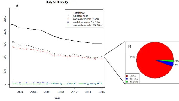
SIH syntheses data (Figure 5.A), show a general decrease of the Bay of Biscay fleet, from 2003 to 2016, that is mainly driven by the diminution of the coastal fleet. This is not surprising given the proportion of coastal vessels in the total French fleet. The coastal vessels were divided into three size classes : less than twelve meters, vessels between twelve and sixteen meters and last class vessels between sixteen and twenty meters. Most of the vessels are less than twelve meters. On average, less than twelve meters vessels represent 94% of coastal vessel (Figure 5B). This proportion is globaly stable between 2006 and 2016. In 2014, the French fleet operating in the coastal area of the Bay of Biscay consists of 1043 vessels, for a total number of 1589 vessels in the bay, mostly less than twelve meters vessels (96% in 2014).
Figure 5. Evolution of vessels repartition depending on their length in the Bay of Biscay (A) and mean repartition of the coastal fleet (B) (data extract from SIH syntheses)
A
17 3.2.2. Representativeness of aerial surveys data
The spatialisation of the fishing pressure is notably based on the aerial surveys data, realized during day time. For the pupose of the sudy we assessed the representativeness of those data. Graphs were produced in order to see what is really observed by those aerial surveys. The number of fishing trips in 2001 was compared between aerial surveys and SIH data.
Generally, there is a higher percentage of towed gears observed. For both passives and towed gears, less than 10% of fishing trips occuring in the Bay of Biscay are recorded. At a smaller scale, disparities are observed at the regional scale, depending on the type of gear and the region. The percentage of fishing trips identifyed in each region is low, varying from 3%, in Brittany for passives gears to 25% for towed gears in Aquitaine.
Figure 6. Comparison of the number of fishing trips between aerial surveys and SIH data for the year 2001
3.2.3. Investigating work hypothesis
One of our work hypotheses was that the spatial occupancy of the fishing vessels, at the scale of the nursery, remained the same between 2001, year of the aerial survey, and in more recent year. This means that the reduction of the fleet observed needed to be equally divided among every fishing zone, e.g. between each region.
The stacked area graph (Figure 7) shows that each region is affected by the decrease of vessels. It also seems that the distribution among regions remained the same on the studied period. Indeed, the contribution of each region to the Bay of Biscay coastal fleet is stable between 2003 and 2016. South of Brittany contributes the most, with 41%, to the coastal fleet, followed by Loire (26%) and Aquitaine (19%) regions. The region Poitou contributes the less with 14% of Bay of Biscay coastal vessels.
Figure 7. Stacked area graph of regional contribution to the coastal fleet between 2003 and 2016
19
3.2.4. Reconstitution of the evolution of the fleets operating in the Bay of Biscay
Using a common gear typology to data extract from SIH syntheses and the access SIH database, the evolution of the fleets operating in the Bay of Biscay was reconstituted from 2001 to 2014. Both general and regional scales were investigated
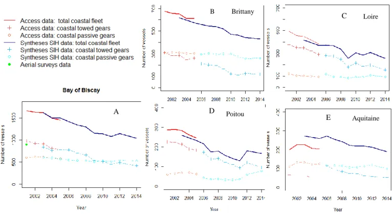
At the scale of the Bay of Biscay (Figure 8.A), we can note that the number of vessels of each gear class for common years are similar for the two datasets. The graph (Figure 8.A) shows a general decline of the number of vessels, for the coastal fleet. It is mostly repercuted on towed gears whereas passive gears are globaly stable over the period. A shift of the type of gear prevailing is observed in 2010. Towed gears used to be predominant before 2010, after what they dropped below passive gears. The same pattern is observed at the regional scale. Globally, the number of towed gears is decreasing whereas passive gears are stable. The reconstruction of fleets evolution seems also corrected at the regionale scale (Figure 8.B, 8.C, 8.D) except for Aquitaine (Figure 8.E) where a general underestimation is underlined. Nevertheless, Poitou-Charentes region shows a slight tendency to increase for the last few years. Finally, the green point (Figure 8.A) that represents the 900 french vessels observed in the Bay of Biscay by the aerial surveys shows that globaly half of the French vessel operating in the coastal zone of the bay of biscay were not observed.
B Brittany Loire Poitou Aquitaine A D E C
Figure 8. Evolution of the Bay of Biscay coastal fleet from 2001 to 2014 using both SIH data sets at the scale of the bay (A) and at the regional scale (B, C, D,E)
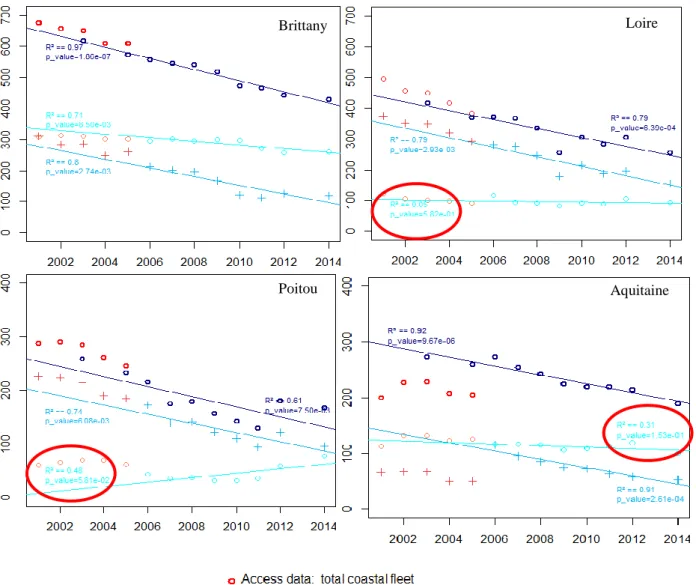
Figure 9. Linear regressions on SIH data extract from the syntheses
3.2.5. Assessing the temporal evolution of the coastal fleets by region
The prediction of the fishing situation in 2014 was assessed using linear regressions were on the data from the SIH syntheses data (e.g. on the time period 2006-2014).
For each region, the evolution of the two types of gears were extracted from the linear regressions. Between 2001 and 2014, towed gears fleet lost 181 vessels in Britanny, 202 in Loire, 111 vessels in Poitou and 96 in Aquitaine. For passive gears, only the regression for the Brittany region was stastically significant, it is the only passive gears fleet affected by a reduction of 75 vessels in 13 years. The percentage of decrease and the number of fishing operations in 2001were retrieved for the 5 significant regressions. The situation in 2014 was then created, for each region and each type of gear.
Brittany
Aquitaine Poitou
21
Then, by combining those results to the geographical positions retrieved from aerial surveys we were able to reconstitute a spatial repartition for the fishing trips that occurred in 2014 (Figure 10.A). Finally, the fishing index was calculated (Figure 10.B)
Figure 10. Geographic positions of coastal vessels reconstituted for 2014 (A) and pressure index due to fishing activity (B)
B A
3.3 Spatialization of data points for chemical contamination and piling
Chemical contamination spatialized according to buffer method considering the three main estuaries as main sources. Results of the spatial extension of the chemical contamination reflect the gradient of nursery sites according to the level of metal or organic contamination. In particular, for organic contamination, the Loire shows the highest scores and the Vilaine the smallest compared to the other nurseries.
Figure 11. Result of the spatialization of pressure index for metal contamination (A) and organic contamination (B)
A B
23 Buffers on pilling points sources impact
For the buffers on piling data, the nursery in the Loire estuary stand out with a higher index of pressure. Both the Vilaine and Pertuis Breton are not affected by this pressure.
Figure 12. Spatialization of the piling index
3.4 Studying contrasts between nurseries: application of the multimetric pressure indicator to the nurseries sites in the Bay of Biscay
To compare and build the indicator, pressure indices were log- transformed and standardized.
Metal contamination and the presence of invasive species seem to be the most variable pressures regardless of the nursery (Figure 13).
3.4.1. Contribution of the different anthropogenic pressures to the multimetric indicator
The six nurseries sites face different level of anthropogenic pressures in term of surfaces impacted as well as number of pressure present in each site. The Bay of Vilaine stands out being exempt of three of the five pressures (piling, aggregate extraction and presence of the slipper limpet) (Table 4).
In term of surface impacted, metal and organic contamination are the most important ones as it diffuses in the water. However, that result is likely due to the spatial extension approach used to diffuse the contamination data. Other approaches as those mentioned earlier should be studied in a sensitivity analysis. Comparing the four other pressures, fishing is the predominant pressure in term of surface impacted.
Table 3. Percentage of surface impacted by each pressure and for each nursery
Global Pressure Indicator (GPI) & Average Level of Pressure j (ALPj)
The GPI was used to compare nurseries sites on their global level of pressure(in black on Figure 15). It is important to note that GPI values don’t reflect the actual values of pressures impacts applied on a nursery. This indicator allows to compare and class nurseries according to their global level of anthropogenic pressure and to identify the nursery with higher exposure. When comparing GPI, the Bay of Bourgneuf, the Gironde and the Pertuis Breton stand out but for opposites reasons. The Gironde and the Bay of Bourgneuf being the most impacted nurseries (respectively with a GPI value of 1038 and 1035) whereas the pertuis Breton has a two time lower GPI (482). The Pertuis Breton is also the only nursery site where fishing pressure contributes the most to the global pressure indicator.
The Average level of a pressure j (ALPj) was used to compare the variation of a pressure between nurseries. The ALP shows the difference of the average level of a pressure from one site to another. But it can reflect the pressure variation intranurseries.
Nursery Vilaine Loire Gironde P.Antioche Bourgneuf P.Breton
Fishing 34 24 36 44 45 51 Metal contamination 100 100 100 100 100 100 Organic contamination 100 100 100 100 100 100 Piling 0 4 5 3 7 1 Aggregate extraction 0 4 2 2 0 0 Invasive species 0 0 0 17 25 11
25
The ALP Contamination has high values for both metal and organic compounds. Contamination is a diffuse pressure that extends to all the surface of the nurceries. That’s why ALPcontamination is higher than the other punctual pressures. Fishing was also found to be the second factor, after metal and organic contaminations, affecting nurseries. It represents an average of 18% of the global pressures affecting nurseries, 75% being already taken by the two contamination indices. The pressure of invasive species, when present in a nursery, contributes more to the GPI of a nursery than both piling and aggregate extraction, two pressures more localized. Those observations are coherent with the previous ones regarding the percentage of surface impacted.
If we compare organic and metal contamination in nurseries, it can be noticed that both Pertuis are more impacted by the organic than metal. Whereas Vilaine nursery presents a higher global level of metal contamination, compare to the organic one. It can be noticed that the decreasing contamiant gradient, imposed by the buffer, appears between the gironde the pertuis Antioche and the pertuis breton. This is not the case for the Loire estuary and the Bay of bourgneuf. The average level of both contaminants is higher in the Bay of Bourgneuf.
Figure 14. Global Pressure Indices (GPI) and Average Level of Pressure (ALP) for each nursery